READ THESE TERMS AND CONDITIONS CAREFULLY BEFORE USING THIS WEBSITE. https://nrc-publications.canada.ca/eng/copyright
Vous avez des questions? Nous pouvons vous aider. Pour communiquer directement avec un auteur, consultez la première page de la revue dans laquelle son article a été publié afin de trouver ses coordonnées. Si vous n’arrivez pas à les repérer, communiquez avec nous à PublicationsArchive-ArchivesPublications@nrc-cnrc.gc.ca.
Questions? Contact the NRC Publications Archive team at
PublicationsArchive-ArchivesPublications@nrc-cnrc.gc.ca. If you wish to email the authors directly, please see the first page of the publication for their contact information.
NRC Publications Archive
Archives des publications du CNRC
This publication could be one of several versions: author’s original, accepted manuscript or the publisher’s version. / La version de cette publication peut être l’une des suivantes : la version prépublication de l’auteur, la version acceptée du manuscrit ou la version de l’éditeur.
Access and use of this website and the material on it are subject to the Terms and Conditions set forth at
Temporary changes in vibrotactile perception during operation of
impact power tools: A preliminary report
Peterson, D.; Brammer, Anthony; Cherniack, M.
https://publications-cnrc.canada.ca/fra/droits
L’accès à ce site Web et l’utilisation de son contenu sont assujettis aux conditions présentées dans le site LISEZ CES CONDITIONS ATTENTIVEMENT AVANT D’UTILISER CE SITE WEB.
NRC Publications Record / Notice d'Archives des publications de CNRC:
https://nrc-publications.canada.ca/eng/view/object/?id=98605f8b-1472-4899-af45-42045561e290 https://publications-cnrc.canada.ca/fra/voir/objet/?id=98605f8b-1472-4899-af45-42045561e290Se
r
TH1
N21d
National Research Consell national10,
1646
1
*
1
Council Canada de recherche= Canadac - 2
Institute for lnstitut deBLDG,
Research in recherche enConstruction construction
P
Modification of Seismic Input for Fully
Discretized Models
by M.O. Al-Hunaidi, I. Towhata and K. lshihara
Reprinted from
Soils and Foundations
Japanese Society of Soil Mechanics and Foundation Engineering Vol. 30, No.
2
June 1990 p. 114-118
(IRC Paper No. 1646)
NRCC 31706
NRC
-
ClSTlt
L I B R A R Y
La methode des elements finis et la solution des 4quations de mouvement dans le domaine temporel servent souvent
ti
l'analyse sismique des problemes d'interaction sol-structures. Dans bien des cas, il est raisonnable de supposer que la base du modele 21 e l h e n t s finis est rigide et, par consequent, d'appliquer la charge sismique sous forme d'accd4rogramme B la base. Les accelerogrammes de base sont calculka
partir des accelerograrnmes temoins disponibles, habituellement enregistres 21 la surface, qui utilisent l'analyse de d6convolution basee sur les modeles continus de sol. Cependant, contrairement aux previsions thhriques, lorsque les acc616rogrammes de d6convolution sont introduits ?I la base du modele ?I elements finis analyse dans le domaine temporel, ils ne reproduisent pas exactement le mouvement temoin initial. Cet Bcart est attribuable aux caracteristiques d'erreur du modele discret, par exemple la frequence de coupure, la dispersion et les reflexions parasites.Les auteurs proposent une methode simple pour resoudre en partie le probleme en modifiant l'acc~l~ronramme de base au-moven d'un modele
unidimensionnd que celles
du modele d'i visqueux
A
la base. On ?antA
laSOILS AND FOUNDATIONS Vol. 30, No. 2, 114-118, June 1990 Japanese Society of Soil Mechanics and Foundation Engineering
TECHNICAL NOTE
MODIFICATION O F SEISMIC INPUT FOR
FULLY
DISCRETIZED MODELS
M. 0. AL-HUNAIDI~), IKUO T O W H A T A ~ ~ ) and KENJI I S H I H A R A ~ ~ ~ )
ABSTRACT
The finite element method together with the solution of the equations of motion in the time domain are often used for seismic analyses of soil-structure interaction problems. In many situations it is reasonable to assume that the base of the finite element model is rigid and hence apply the seismic loading in the form of an accelerogram at the base. Base accelerograms are calculated from available criteria accelerograms, usually recorded at the surface, employing deconvolution analysis based on continuum soil models. However, contrary to theoretical pre- dictions, when the deconvolved accelerograms are input at the base of the finite element model analyzed in the time domain, they do not exactly reproduce the original criteria motion. This discrepancy is attributed to the error characteristics of the discretized model such as cut-off frequency, dispersion and spurious reflections.
A simple method is proposed to partly overcome this problem by modifying the base accelero- gram employing a one-dimensional soil model which has the same error characteristics as those of the interaction model. This model employs a viscous dashpot at the base. Vertically pro- pagating shear waves are considered.
Key words : computer application, dynamic, earthquake, finite element method, wave propagation (IGC: E 8)
that the base of the finite element model is INTRODUCTION rigid and hence to apply the seismic loading The finite element method together with the in the form of an accelerogram at the base. numerical solution of the equations of motion Base accelerograms are determined from avail- in the time domain are often used for seismic able criteria accelerograms, usually recorded analyses of soil-structure interaction problems. at the surface, using deconvolution analysis In many situations, it is reasonable to assume based on continuum soil models. Contrary to
i) Research Associate, Institute for Research in Construction, National Research Council of Canada, Ottawa, Ontario, Canada KIA 0R6.
ii) Associate Professor of Civil Engineering, University of Tokyo, Bunkyo-ku, Tokyo 113.
iii) Professor of Civil Engineering, University of Tokyo, Bunkyo-ku, Tokyo 113. Manuscript was received for review on April 17, 1989.
Written discussions on this note should be submitted before January 1, 1991, to the Japanese Society of Soil Mechanics and Foundation Engineering, Sugayama Bldg. 4 F, Kanda Awaji-cho 2-23, Chiyoda- ku, Tokyo 101, Japan. Upon request the closing date may be extended one month.
MODIFICATION OF SEISMIC INPUT 115
theoretical predictions, however, when accelero- grams are input at the base of the finite element mesh without the structure, they do not exactly reproduce the original criteria
motion at the surface. This is because of
one or more of the following factors:
Upper limit of frequency that a mesh can reproduce accurately
Dispersion characteristics of the finite elements
Spurious reflections due to mesh gradation Dispersion and accuracy characteristics of the time integration schemes
In the following sections a simple method is proposed to partly overcome this problem by modifying the base accelerogram using a one dimensional soil model having the same error characteristics as those of the interaction model. The one dimensional model, however, has a viscous dashpot attached to its base. Vertically propagating shear waves are considered.
1-D SHEAR WAVE PROPAGATION For vertically propagating shear waves in an elastic homogeneous medium, the horizontal displacement u, a function of time t and depth x , is governed by the following partial differ- ential equation
aZu/at2
-
v s 2 a z u l a 2 = o ( 1 )where Vs= dG/p=shear wave velocity, G
and p are the material shear modulus and density, respectively. The general solution of
Eq. (1) for harmonic motion of frequency o
can be expressed as
U(X, t) = E exp[i(kx+ ot)]
+Fexp[-i(kx-ot)] ( 2 )
and the corresponding shear stress is
r (x, t ) = pVsio[E exp(ikx)
+Fexp(-ikx)] exp(iot) ( 3 )
where k=o/Vs=wave number. For a hori-
zontally layered medium, Eqs. (2) and (3) are
valid for each layer and x becomes the local
depth coordinate of the layer. Coefficients E
and F are determined by satisfying the zero
stress condition at the free surface and dis- placement and stress continuity at layer inter-
faces. This results in a closed form recursive solution like that implemented in the well
known computer program SHAKE developed
by Schnabel et al. (1972). Transient motions can be handled by the Fourier transform technique.
In Eq. (2) the first term represents a wave traveling in the negative x-direction (upward)
and is called the incident wave I; the second
term represents a wave traveling in the posi- tive x-direction (downward) and is called the
reflected wave R. Kunar and Rodrigues (1980)
explain the physical meaning of these two parts when they are used as a rigid-base input
accelerogram as follows :
The incident component I propagates up-
wards to the surface to reproduce the criteria motion. Then it is reflected back
towards the base (note : the incident part
which is on its way from the surface back to base is in fact what is called the re- flected part in Eqs. (2) and (3)).
When the incident component arrives back at the base, it is reflected back to the surface with the same magnitude but with opposite sign.
The incident part reflected at the base, however, does not propagate back to the surface because it cancels out with the
reflected component R of the base input
which is of equal but opposite magnitude. The problem of concern here is that when base accelerograms obtained by deconvolution procedures, which usually employ continuum models, are used as input for discretized
models, the following error is introduced : The
incident component of the input I is distorted
while propagating up and down in the dis- cretized model and consequently it does not cancel out exactly with the reflected component
R of the input. This, in turn, produces a
surface motion different from the original criteria motion.
The distortion in the incident part of the motion is mainly due to the dispersion char- acteristics of the space and time discretizations employed. Fig. 1 shows dispersion curves for the one-dimensional, constant strain finite element in conjunction with some time integra-
116 AL-HUNAIDI ET AL.
2 (element size) l (wave length)
Fig. 1 Dispersion curves of the constant strain line element (Lumped mass) with time in- tegration performed using Newmark's @
scheme : @= 0 (central difference scheme) ;
@=1/4 (trapezoidal method) at different Courant numbers C (after Belytschko and Mullen, 1978)
tion schemes (after Belytschko and Mullen, 1978).
The vertical axis of Fig. 1 represents the ratio between the wave speed in the discretiz- ed system and that in the continuum ; whereas the horizontal axis represents the ra,tio between the element size and the wave length (note :
multiplying this ratio by 2 is done to scale the horizontal axis between 0 and 1 as the allowable value for this ratio should not exceed 1/2). In Fig. 1 also, the Courant number, C, is defined as C= At (wave velocity)/(element size), where At is the size of the time incre- ment. The curve marked as Exact time in- tegration refers to the semi-discretized case in which only space discretization is performed; no time discretization is performed, i.e. time integration errors are not present.
In the following section a simple method is proposed to modify base accelerograms so that incident waves reflected off the free surface are cancelled at the base by the reflected part of the input motion.
MODIFICATION PROCEDURE
--
*
(a) (b)
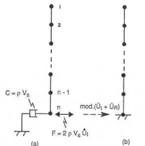
Fig. 2. Half-space model uging constant strain line element with (a) viscous base (b) fixed base
of the soil model, only the incident part of the input accelerogram is required ; the reflected part must be omitted. The incident part will be absorbed by the dashpots after it is reflected off the free surface. In the case of vertically propagating shear waves, Joyner and Chen (1975) have shown that the dashpot coefficient is pVs and the seismic loading is applied in the form of an effective stress 2 ~ V S U I , as shown in Fig. 2 for the half-space modeled by line elements. UI is the particle velocity for the incident wave at the base. This actually corresponds to applying an accelero- gram equal to twice the incident part in Eq.
(2) at the fixed end of the dashpot. Then the problem can be stated in terms of relative motion between the free nodes and the fixed end of the dashpot as follows
[MI [ar}
+
[C] IvT}+
[K] Idr} = -[MI {2 UI}( 4
where
[m,
[C] and [K] are the mass matrix, damping matrix and stiffness matrix, respec- tively; {ar], {vr} and { d ~ ] are the relative acceleration, velocity and displacement vectors, respectively. UI is the particle acceleration for the incident wave. Absolute motion is obtained by adding 2 UI, 2 UI, 2 UI to the relative motion dr, vT, aT, respectively.If mace and time discretizations used for If viscous dashpots are attached to the base the one-dimensional soil model with viscous
MODIFICATION OF SEISMIC INPUT 117
dashpots at the base are exactly the same as those used for the two or three-dimensional soil-structure model, then the response at node (n) in Fig. 2 (a) is the desired modified base motion. When this modified base motion is used for the soil column but without the dashpot, the incident and reflected parts will cancel, almost exactly, as demonstrated by the numerical examples in the next section. In summary, the modification procedure consists of the following steps :
1. Perform a deconvolution analysis, using the SHAKE program for instance, to obta.in the base incident motion UI that corresponds to the given surface motion.
2. Run a one dimensional model analysis using the base input 2 UI in order to obtain the modified base input mod. (UI
+
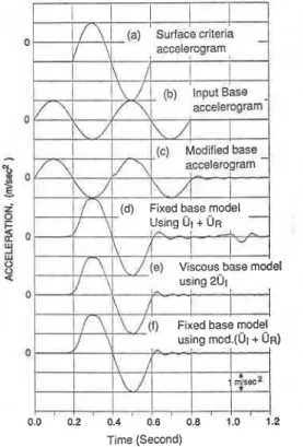
UR). The one dimensional model should employ a viscous bottom boundary and it should have the same space and time discretizations used for the0 (a) Surlace cdterla
accelerogram ,
(c) Modlflad base
(d) Fixed base model Us~ng 01 + SIR
(e) Viscous-base model
m!
using mod.(U~ + UR)
, .
0.0 0.2 0.4 ' 0.6 ' 0.8 ' 1.0 1.2
Time (Second)
Fig. 3. Acceleration input and output results of example (1) using Newmark's time inte- gration method
soil-structure interaction model.
3. Run the two or three dimensional model
of the problem at hand with a rigid base at which the specified motion is given by mod. (UI+ UR).
VERIFICATION EXAMPLES
For vertically propagating shear waves with planar wave front, the half-space can be model- ed by a series of line elements. In the fol- lowing analyses, one-dimensional constant strain line elements are employed as shown in Fig. 2. Each element has length 4 m, cross- sectional area 1 m2, density 1.8 t/m3 and shear modulus 288000 kN/m2. A total of 20 elements are used and lumped mass formulation is adopted. The seismic loading is input in the form of an accelerogram at the fixed base. All computations were performed in double precision.
Fig. 3 presents the input and results of the first example as follows :
(a) Criteria surface acceleration : one cycle sine wave with period T = 2 H/Vs =0.4s, where H is the depth to the fixed base.
(b) Exactly deconvolved base acceleration
UI
+
UR
(c) Modified base acceleration as proposed mod. (
UI
+
UR)(d) Surface output acceleration using dis- cretized fixed base model and exactly decon- volved base accelerogram UI
+
UR(e) Surface output acceleration using dis- cretized model with viscous base and the in- cident part of the exactly deconvolved base accelerogram 2
UI
(f) Surface output acceleration using dis- cretized fixed base model and modified base accelerogram mod. (
UI
+
UR)Newmark's time integration scheme (Bathe and Wilson, 1976) is used with the following parameters : ,8 =0.25,
r
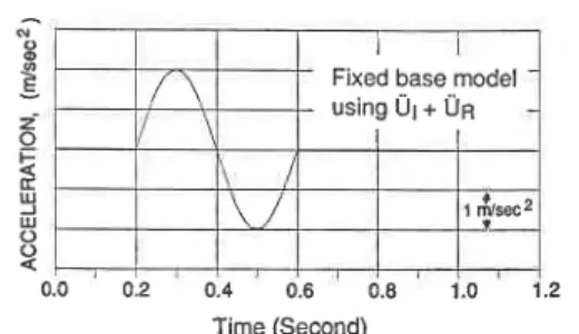
=0.5 and time step A t = 0.01 second. Comparison of curves (d) and (f) in Fig. 3 indicates the improvement of output surface acceleration by using the modi- fied base accelerogram.The same problem presented above is solved again but using the central difference time
118 AL-HUNAIDI ET AL.
Time (Second)
Fig. 4. Output surface acceleration using central difference time integration with Courant number = 1
integration scheme (Bathe and Wilson, 1976). W i t h Courant number C=1.0 and lumped mass formulation, this discretized system is completely non-dispersive (see Fig. 1). Fig.
4 shows the surface output acceleration of the fixed base model using the unmodified base accelerogram UI
+
UR. T h e output is exactly the same as the criteria surface acceleration. Although this example applies only to one- dimensional wave propagation using linear displacement elements in a uniform mesh and time integration with Courant number C= 1.0, the results demonstrate that a satisfactory time history can be obtained when wave distortionFig. 5. Output surface acceleration of example (2) using Newmark's time integration method
is prevented.
In the second example, SHAKE program (Schnabel et al., 1972) is used to deconvolve the first 10 seconds of the EL CENTRO earth- quake (frequencies above 10 Hz are removed). T h e resulting base accelerogram is then ap- plied to the half-space model used in the first example. T h e surface output acceleration is shown in Fig. 5 for the following models:
(a) Discretized fixed base model using un- modified SHAKE output base accelerogram
U I uR.
(b) Discretized model with viscous base using the incident part of SHAKE output base accelerogram 2 U I .
(c) Discretized fixed base model using modified SHAKE output base accelerogram
mod. (UI ir+ UR).
Comparison of curves (a) and (c) in Fig. 5
demonstrates the advantage of the proposed modification procedure for the base accelero-
gram.
I
I
I
REFERENCES
1) Bathe, K. and Wilson, W. L. (1976): Numeri- cal Methods in Finite Element Analysis, Pren- tice-Hall Inc., Englewood Cliffs, New Jersey, pp. 308-344.
2) Belytschko, T. and Mullen, R. (1978) : "On dis- persive properties of finite element solutions," Modern Problems of Elastic Wave Propagation, J. Miklowitz and J. D. Achenbach, eds., John Wiley and Sons Inc., pp. 67-82.
3) Joyner, W. B. and Chen, A. T. F. (1975): "Cal- culation of nonlinear ground response in earth- quakes," Bul. of the Seism. Soc. of America, 65(5), pp. 1315-1336.
4) Kunar, R. R. and Rodriguez-Ovejero, L. (1980) :
"A model with nonrdecting boundaries for use in explicit soil-structure interaction analyses," Earthquake Engineering and Structural Dy- namics, 8(3), pp. 361-374.
5) Schnabel, P. B., Lysmer, J. and Seed, H. B. (1972) : "SHAKE : a computer program for earth- quake response analysis of horizontally layered sites," Report No. EERC 72-12, Earthquake Engineering Research Center, Univ. of California, Berkeley, Calif.