HAL Id: hal-00726767
https://hal.archives-ouvertes.fr/hal-00726767
Submitted on 31 Aug 2012
HAL is a multi-disciplinary open access
archive for the deposit and dissemination of
sci-entific research documents, whether they are
pub-lished or not. The documents may come from
teaching and research institutions in France or
abroad, or from public or private research centers.
L’archive ouverte pluridisciplinaire HAL, est
destinée au dépôt et à la diffusion de documents
scientifiques de niveau recherche, publiés ou non,
émanant des établissements d’enseignement et de
recherche français ou étrangers, des laboratoires
publics ou privés.
More efficient periodic traversal in anonymous
undirected graphs
Jurek Czyzowicz, Stefan Dobrev, Leszek Gąsieniec, David Ilcinkas, Jesper
Jansson, Ralf Klasing, Ioannis Lignos, Russell Martin, Kunihiko Sadakane,
Wing-Kin Sung
To cite this version:
Jurek Czyzowicz, Stefan Dobrev, Leszek Gąsieniec, David Ilcinkas, Jesper Jansson, et al.. More
efficient periodic traversal in anonymous undirected graphs. Theoretical Computer Science, Elsevier,
2012, 444, p. 60-76. �10.1016/j.tcs.2012.01.035�. �hal-00726767�
More efficient periodic traversal in
anonymous undirected graphs
✩Jurek Czyzowicza, Stefan Dobrevb, Leszek G ֒
asieniecc,1, David Ilcinkasd,2, Jesper Janssone,3,
Ralf Klasingd,2, Ioannis Lignosf, Russell Martinc,4, Kunihiko Sadakaneg, Wing-Kin Sungh
aD´epartement d’Informatique, Universit´e du Qu´ebec en Outaouais, Gatineau, Qu´ebec J8X 3X7, Canada. bInstitute of Mathematics, Slovak Academy of Sciences, Dubravska 9, P.O.Box 56, 840 00, Bratislava, Slovak Republic.
cDepartment of Computer Science, University of Liverpool, Ashton Street, Liverpool, L69 3BX, United Kingdom. dLaBRI, CNRS and University of Bordeaux, 351 cours de la Liberation, F-33405 Talence cedex, France.
eOchanomizu University, 2-1-1 Otsuka, Bunkyo-ku, Tokyo 112-8610, Japan.
fDepartment of Computer Science, Durham University, South Road, Durham, DH1 3LE, United Kingdom. gPrinciples of Informatics Research Division, National Institute of Informatics, 2-1-2 Hitotsubashi, Chiyoda-ku,
Tokyo 101-8430, Japan.
hDepartment of Computer Science, National University of Singapore, 3 Science Drive 2, 117543 Singapore.
Abstract
We consider the problem of periodic graph exploration in which a mobile entity with constant memory,
an agent, has to visit all n nodes of an input simple, connected, undirected graph in a periodic manner.
Graphs are assumed to be anonymous, that is, nodes are unlabeled. While visiting a node, the agent may distinguish between the edges incident to it; for each node v, the endpoints of the edges incident to v are uniquely identified by different integer labels called port numbers. We are interested in algorithms for assigning the port numbers together with traversal algorithms for agents using these port numbers to obtain short traversal periods.
Periodic graph exploration is unsolvable if the port numbers are set arbitrarily, see [1]. However, sur-prisingly small periods can be achieved by carefully assigning the port numbers. Dobrev et al. [4] described an algorithm for assigning port numbers and an oblivious agent (i.e., an agent with no memory) using it, such that the agent explores any graph with n nodes within the period 10n. When the agent has access to a constant number of memory bits, the optimal length of the period was proved in [7] to be no more than 3.75n − 2 (using a different assignment of the port numbers and a different traversal algorithm). In this paper, we improve both these bounds. More precisely, we show how to achieve a period length of at most (4 +1
3)n − 4 for oblivious agents and a period length of at most 3.5n − 2 for agents with constant
memory. To obtain our results, we introduce a new, fast graph decomposition technique called a three-layer
partition that may also be useful for solving other graph problems in the future. Finally, we present the
first non-trivial lower bound, 2.8n − 2, on the period length for the oblivious case.
Keywords: algorithms and data structures, graph exploration, periodic graph traversal, oblivious agent,
1. Introduction
Efficient search in unknown or unmapped environments is a fundamental problem in algorithmics. Its applications range from robot navigation in hazardous environments to rigorous exploration (and indexing) of data available on the Internet. Due to a strong need to design simple and cost-effective agents as well as to design exploration algorithms suitable for rigorous mathematical analysis, it is of practical importance to limit the memory of agents.
In this paper, we consider the task of graph exploration by a mobile entity equipped with a constant number of bits memory. The mobile entity may be, e.g., an autonomous piece of software navigating through a graph that represents the nodes and connections of a computer network. For the sake of simplicity, we call the mobile entity an agent and model it as a finite state automaton. We require that the agent visits all nodes in an input graph infinitely many times, in a periodic manner. The task of periodic traversal of all nodes of a network is particularly useful in network maintenance, where the status of every node has to be checked regularly.
To assist the agent, we assign local port numbers to the edges at each node as a preprocessing step. Then, while traversing the graph, the agent is allowed to use the local port numbers to ensure that all nodes are visited. Our goal is to minimize the length of the traversal period; in other words, we would like to assign the port numbers so that the maximum number of edge traversals performed by the agent between two consecutive visits to the same node and entering through the same port is minimized. From here on, we assume that the input graph is simple, connected, and undirected. We also assume it to be anonymous, i.e., all nodes are unlabeled.
1.1. Problem definition
Let G = (V, E) be a simple, connected, undirected graph. For any node v ∈ V , the degree of v is the number of neighbors of v and is denoted by dv. To enable an agent to distinguish between the different
edges incident to a node, the edges at every node v will be assigned local port numbers from {1, 2, . . . , dv}
bijectively. (Every edge will therefore be assigned two port numbers; one at each of its two endpoints.) See Figure 1.
We model agents as Mealy automata. The Mealy automaton has a finite number of states and a transition function f governing the actions of the agent (cf. [10]). If the automaton enters a node v of degree dvthrough
port i in state s, it switches to state s′ and exits the node through port i′, where (s′, i′) = f (s, i, d v). The
memory size of an agent is related to its number of states; to be precise, it equals the number of bits needed to encode these states. Note that in this model, the size of the agent’s memory represents the amount of information that the agent can remember while moving. This does not restrict computations made on a node and thus the transition function can be any deterministic function; any additional memory needed for computations can be seen as provided temporarily by the hosting node. Nevertheless, our traversal algorithms only perform very simple tests and operations on the non-constant inputs i and d, namely equality tests and incrementations.
✩A preliminary version of this article appeared in Proceedings of the 16th
International Colloquium on Structural Information and Communication Complexity(SIROCCO 2009), vol. 5869 of Lecture Notes in Computer Science, Springer-Verlag, pp. 174– 188, 2009.
Email addresses: [email protected](Jurek Czyzowicz), [email protected] (Stefan Dobrev),
[email protected](Leszek Gasieniec), david.ilcinkaslabri.fr (David Ilcinkas), [email protected]֒ (Jesper Jansson), [email protected] (Ralf Klasing), [email protected] (Ioannis Lignos),
[email protected] (Russell Martin), [email protected] (Kunihiko Sadakane), [email protected] (Wing-Kin Sung)
1
Partially funded by the Royal Society International Joint Project, IJP - 2007/R1. 2
Supported in part by the ANR projects ALADDIN and ALPAGE, the INRIA project CEPAGE, and the European projects GRAAL and DYNAMO.
3
Funded by the Special Coordination Funds for Promoting Science and Technology, Japan. 4
Partially funded by the Nuffield Foundation grant NAL/32566, “The structure and efficient utilization of the Internet and other distributed systems”.
v d −1 dv 2 3 1
Figure 1: In a port number assignment, the dv edges incident to node v are locally given the numbers 1, 2, 3, . . . , dvin some order.
The problem considered in this paper is to design a port number assignment algorithm and a traversal algorithm that enable the agent to periodically visit all nodes in an input graph. The efficiency measure we use to compare solutions is the resulting period length, which is the maximum number of edge traversals between two consecutive visits to a node entering through the same port, taken over all nodes. The period length is expressed in terms of n, the number of nodes in the input graph, and our main objective is to find algorithms achieving a small period length for any input graph. We focus on two cases: the oblivious agent, having a single state (or equivalently, zero memory bits), and the constant-memory agent, equipped with a constant number of bits independent of the size of the input graph. By the above discussion, oblivious agents can be regarded as having access to any amount of temporary memory while stationed at a node but losing all this memory when exiting the node.
1.2. Previous results
Budach [1] proved that no finite automaton can explore all graphs. Rollik [12] later proved that an agent needs Ω(log n) memory bits to explore any graph with n nodes, even if restricted to cubic planar graphs. (This lower bound was in fact recently proved to be optimal by Reingold in his breakthrough paper [11].) Therefore, the basic periodic graph exploration problem is unsolvable for agents with small memory. Providing the agent with a pebble to mark nodes does not help much as the asymptotic size of the memory needed remains Ω(log n) bits [5]. Furthermore, even a highly-coordinated multi-agent team capable of (restricted) teleportation cannot explore all graphs using only constant memory [3]. Nevertheless, placing some extra information in the graph can help a lot. Cohen et al. [2] demonstrated that putting two bits of advice at each node allows any graph to be explored by an agent with constant memory by a periodic traversal of length O(m), where m is the number of edges.
The impossibility results mentioned above all use the ability of an adversary to assign local port numbers in a misleading order. On the other hand, if port numbers are carefully assigned beforehand (still under the condition that at each node v, port numbers from 1 to dv are employed) then a simple agent, even an
oblivious one, can perform periodic graph exploration within a period of length O(n) [4]. More precisely, Dobrev et al. [4] showed that there exists an algorithm for setting the port numbers in such a way that an oblivious agent using the so-called Right-Hand-on-the-Wall algorithm as its traversal algorithm will traverse any graph with n nodes within the period 10n. Significantly, this holds even if the nodes themselves are not marked in any way while the agent traverses the graph. For agents with constant memory, Ilcinkas [8] gave an algorithm achieving an upper bound of 4n − 2 on the period length, which was subsequently improved to 3.75n − 2 by Gasieniec et al. [7]. (References [4] and [8] also considered dynamic versions of periodic graph֒ exploration in which the graph may be modified while the agent is traversing it.)
As for corresponding lower bounds on the period length, the star graph with n nodes (i.e., having n − 1 edges) yields a trivial lower bound of 2n − 2 for any type of agent, independent of the amount of available memory, since every edge of the graph must be traversed in both directions. Also note that in case the input graph contains a Hamiltonian cycle, the optimal period length is n: just set the port numbers to direct the agent along the cycle.
1.3. Our new results and organization of the paper
In this paper, we improve the previously best upper and lower bounds on the period length for periodic graph exploration by an oblivious agent [4] and by an agent with constant memory [7, 8] as follows. We present an efficient deterministic algorithm named FindWitnessCycle for assigning port numbers at the nodes of the input graph so that an oblivious agent using an extremely simple traversal algorithm named the Right-Hand-on-the-Wall algorithm (reviewed in Section 2.2) achieves a period length of at most (4 + 1
3)n − 4. Our port number assignment algorithm relies on a new three-layer partition technique for
graphs, described in Section 3, permitting an optimal O(|E|)-time construction of the port labeling. The details of FindWitnessCycle can be found in Section 4. As a special case, we also consider a class of graphs for which an oblivious agent can obtain a traversal with period length at most 2n by using a simpler algorithm named TerseCycles as the port number assignment algorithm. Next, we provide the first non-trivial lower bound, 2.8n− 2, on the period length for oblivious agents in the general case in Section 5. Then, in Section 6, we give an algorithm (also based on the three-layer partition approach) which assigns port numbers so that an agent with constant memory is able to accomplish periodic graph exploration within a period length of at most 3.5n − 2. Finally, Section 7 summarizes our new results and discusses some related open problems.
2. Preliminaries
2.1. Notation and basic definitions
For any undirected graph G = (V, E), we denote by −→G the symmetric directed graph obtained from G by replacing each undirected edge {u, v} ∈ E by two directed edges in opposite directions: one directed edge from u to v, denoted by (u, v), and one directed edge from v to u, denoted by (v, u). For each directed edge (u, v) or (v, u), we say that the undirected edge {u, v} ∈ G is its underlying edge. For any node v of a directed graph the out-degree of v is the number of directed edges leaving v, the in-degree of v is the number of directed edges incoming to v, and cumulative degree of v is the sum of its out-degree and its in-degree.
Directed cycles constructed by our algorithm traverse some edges in G once and other edges twice (in opposite directions). However, at early stages, our algorithm for oblivious agents is solely interested in whether the edge is unidirectional or bidirectional, regardless of the direction. To alleviate the presentation (despite some abuse of notation), in this context, an edge that is traversed once when deprived of its direction is called a one-way edge. Similarly, an edge that is traversed twice is called a two-way edge, and it is understood to be composed of two one-way edges. Hence, we extend the notion of one-way and two-way edges to general directed graphs in which the direction of edges is removed. In particular, we say that two nodes s and t are connected by a two-way path, if there is a finite sequence of nodes v1, v2, . . . , vk, where
each pair vi and vi+1 is connected by a two-way edge, and s = v1 and t = vk.We call a directed graph
− → K
two-way connected if for any pair of nodes there is a two-way path connecting them. Note that two-way
connectivity implies strong connectivity, but not the other way around.
2.2. Traversal algorithms for oblivious agents
A simple graph traversal algorithm for oblivious agents is the Right-Hand-on-the-Wall algorithm [4]. This algorithm is specified by the transition function f : (s, i, d) 7→ (s, (i mod d) + 1). Differently speaking, if the agent enters a degree-dv node v by port number i, it will exit v through port number (i mod dv) + 1.
The Right-Hand-on-the-Wall algorithm assumes that the initial starting node can be any node v in G and that the agent entered v from port number dv; therefore, the traversal will always start with an edge with
port number 1. See Figure 2 for an example. For any given graph, there exists at least one assignment of port numbers that allows the Right-Hand-on-the-Wall algorithm to visit all nodes periodically [4].
Graph traversal according to the Right-Hand-on-the-Wall algorithm is called right-hand traversal or
RH-traversal for short.
Given a port number assignment algorithm and a traversal algorithm for the agent, it is possible, for a given degree d, to permute all port numbers incident to each degree-d node of a graph G according to some
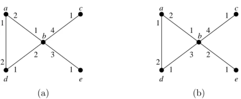
1 2 1 1 1 2 1 3 4 b d a e c 2 1 2 1 1 1 2 1 3 2 4 b d a e c (a) (b)
Figure 2: (a) Running the Right-Hand-on-the-Wall algorithm with the given port number assignment and starting at node a will visit all nodes of the graph in the order ha, d, b, e, b, c, b, a, . . . i, with period length 7. (b) If this port number assignment is used then the Right-Hand-on-the-Wall algorithm will not be able to visit all nodes of the graph.
fixed permutation σ, and to modify the transition function f of the agent accordingly, so that the agent behaves exactly the same as before in G. The new transition function f′ is in this case given by the formula
f′ = σ ◦ f ◦ σ−1 and the two traversal algorithms are said to be equivalent. More precisely, two traversal
algorithms described by their respective transition functions f and f′ are equivalent if for any d > 0 there
exists a permutation σ on {1, . . . , d} such that f′ = σ ◦ f ◦ σ−1. The following lemma states that any pair
consisting of a port number assignment algorithm and a traversal algorithm for oblivious agents, and solving the periodic graph exploration problem, can be expressed by using the Right-Hand-on-the-Wall algorithm as the traversal algorithm.
Lemma 1. Any traversal algorithm enabling an oblivious agent to explore all graphs is equivalent to the
Right-Hand-on-the-Wall algorithm.
Proof. Consider an arbitrary algorithm A enabling an oblivious agent to periodically explore all graphs. Let
f be its transition function. Fix an arbitrary d > 1 and let fd be the function i 7→ f (s, i, d) from {1, . . . , d}
to {1, . . . , d}, where s is the single state of the oblivious agent. Consider the d + 1-node star of degree d. For 1 ≤ i ≤ d, let vi be the leaf reachable from the central node u by the edge with port number i.
For the purpose of obtaining a contradiction, first suppose that fd is not surjective. Let i be a port
number without pre-image. If the agent is started by the adversary in node vj, with j 6= i, then the node
vi is never explored. Therefore fd is surjective, and thus a permutation of the set {1, . . . , d}. Again for the
purpose of contradiction, suppose that fd can be decomposed into more than one cycle. Let i be a port
number outside 1’s orbit (i.e., 1 and i are not in the same cycle of the permutation). If the agent is started by the adversary in node v1, then the node vi is never explored. Hence, fd is a cyclic permutation, i.e.,
it is constructed with a single cycle. Since the equivalence classes of permutations (often called conjugacy classes) correspond exactly to the cycle structures of permutations, the traversal algorithm A is equivalent to the Right-Hand-on-the-Wall algorithm.
Because of Lemma 1, we will always assume in the rest of the paper when referring to oblivious agents that the Right-Hand-on-the-Wall algorithm is employed as the traversal algorithm.
2.3. Witness cycles and RH-traversability
Any (possibly non-simple) directed cycle formed when traversing a graph according to the Right-Hand-on-the-Wall algorithm described above for a fixed port number assignment is called an RH-cycle. A witness
cycle for a graph G is an RH-cycle that contains every node of G at least once.
If we are given a witness cycle C for G, it is straightforward to assign port numbers to the nodes in G so that an oblivious agent using the Right-Hand-on-the-Wall algorithm will traverse G according to C. (To ensure that any node can be used as the starting node, at every node v, assign port numbers 1 and dvto an
underlying edge for an edge in C directed out from v and into v, respectively.) Therefore, to obtain a port number assignment algorithm for oblivious agents, we just need to specify how to construct a witness cycle for any input graph. This will be done in Section 4.
One key step in our method in Section 4 is to compute a set of RH-cycles and then merge them into a single witness cycle. Recall that −→G is the symmetric directed graph obtained from G by replacing each undirected edge by two directed edges. In the rest of this subsection, we characterize when a spanning subgraph of−→G is a union of RH-cycles.
Definition 1. Let −→H be a spanning subgraph of−→G. A node v ∈ G is RH-traversable in −→H if there exists a port number assignment π for G such that, for each edge (u, v) ∈−→H incoming to v via an underlying edge e, there exists an outgoing edge (v, w) ∈−→H leaving v via an underlying edge e′ such that e′ is the successor of e in π at node v.
As a special case, if−→H is a witness cycle for G then every node is RH-traversable in−→H. However, nodes may be RH-traversable in−→H even if−→H is not a witness cycle (q.v. Figure 4), and the next lemma (Lemma 2) gives a useful condition for checking RH-traversability in the general case. To state the lemma, we need the following additional notation. Let−→H be a fixed spanning subgraph of−→G. Any undirected edge {u, v} in G is called a two-way edge for −→H if both of the directed edges (u, v) and (v, u) belong to −→H. Otherwise, if (u, v) belongs to−→H but (v, u) does not, then {u, v} is called a one-way edge to v in−→H as well as a one-way
edge from u in−→H. For each node v in−→H, define: • bv = The number of two-way edges for
− →
H incident to v. • iv = The number of one-way edges to v in
− → H. • ov = The number of one-way edges from v in
− → H.
Thus, bv+ iv+ ov equals the number of edges in G incident to v that are underlying edges for directed edges
belonging to−→H. For an example, see Figure 3.
Lemma 2. A node v is RH-traversable in−→H if and only if bv= dv or iv= ov>0.
Proof. (⇒) Let π be a port number assignment for G meeting the requirements of Definition 1 and denote
the port number assigned by π to any edge e at v by π(e). If bv = dv then we are done, so consider the
case bv 6= dv. Suppose for the sake of contradiction that there are no one-way edges to v or from v. Let e
be any edge that is not two-way and let e′ be the two-way edge with the largest possible π(e′) satisfying
π(e′) < π(e). It follows that there must exist some one-way edge f from v with π(e′) < π(f ) < π(e), which
is a contradiction. Therefore, there exists at least one-way edge to v or from v, and thus iv>0 or ov >0 by
definition. The number of incoming edges equals the number of outgoing edges at v, so bv+ iv = bv+ ov,
i.e., iv= ov.
(⇐) If bv = dv then all edges incident to v are used in both directions and any ordering of the edges
gives an acceptable port number assignment. Otherwise, bv 6= dv and iv = ov > 0, and we can take the
following port number assignment: First, all underlying edges that are two-way edges for−→H are numbered consecutively, starting from 1, followed by an underlying edge for any one-way edge from v. Next, all other underlying edges for one-way edges are numbered consecutively while alternating between one-way edges to v and one-way edges from v so that the last (incoming) edge gets port number dv. See Figure 3. Finally,
the remaining edges may be numbered arbitrarily by the unused port numbers. Lemma 2 immediately yields:
Corollary 1. A spanning subgraph−→H of −→G is a union of RH-cycles if and only if at each node v of G, the number of one-way edges to v in−→H equals the number of one-way edges from v in−→H, and if this number is zero then all two-way edges for −→G incident to v must also be present in−→H.
2
1
v3
d
d −1
v v vd −2
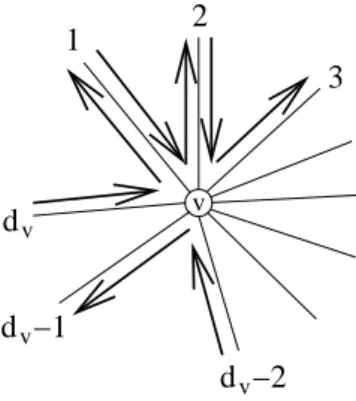
Figure 3: In this example, edges belonging to−→H are shown as arrows. Node v has dv> bv = 2, iv = 2, and ov= 2, so by Lemma 2, v is RH-traversable in−→H. The displayed port number assignment corresponds to the construction in the proof of Lemma 2.
2.4. Operations on cycles by modifying port numbers
Consider the graph and the port number assignment in Figure 4. The port numbers induce a set C of three RH-cycles. Every node is RH-traversable in the directed graph formed by taking the union of the cycles in C according to Lemma 2, but there is no witness cycle in C. However, if we exchange two port numbers at one of the degree-three nodes, then the three cycles merge into a witness cycle.
In this subsection, we describe two operations on cycles (implemented by modifying the corresponding port number assignments) and the conditions under which these operations will produce a witness cycle. The operations are called Merge3 and EatSmall, and were introduced by Dobrev et al. in [4].
1 1 2 1 2 2 2 1 1 2 3 2 3 1
Figure 4: The above port number assignment induces three cycles, indicated by dashed and dotted lines. Note that every node is RH-traversable in the union of the three cycles, but there is no witness cycle among the three cycles.
Let−→H be a subgraph of G that has only RH-traversable nodes. Observe that any port number assignment partitions−→H into a set of RH-cycles. Take any ordering γ of this set of cycles. We define two rules which transform one set of cycles to another by changing the port number assignment. The first rule, Merge3, takes as input three cycles incident to a node and merges them into one cycle. In the case where the node is visited by more than three cycles, the rule is applied to arbitrarily chosen three cycles. The second rule,
EatSmall, breaks a non-simple cycle into two subcycles and transfers one such subcycle to another cycle.
• Rule Merge3: Let v be a node incident to at least three different cycles C1, C2and C3. Let x1, x2
and x3be the underlying edges at v containing incoming edges for cycles C1, C2and C3, respectively
(x1, x2 and x3 can be a one-way edge or a two-way edge in
− →
H). Assume w.l.o.g. that x2 is between
x1and x3 in the port number assignment at v; see Figure 5. Modify the port number assignment at v
as follows: (1) let the successor of x2 become the new successor of x1, (2) let the old successor of x3
(4) keep the same relative order of the other edges. It is easy to see that this operation connects the cycles C1, C2 and C3 into a single cycle.
3 4 6 1 2 3 4 5 6 C1 C2 C3 before after 1 = x1 2 = x2 5 = x3 C3
Figure 5: Applying rule Merge3 will change the port number assignment at the shown node so that the three cycles C1, C2, and C3 are merged into one cycle.
• Rule EatSmall:
Let C1be the smallest cycle in the ordering γ such that
– there is a node v that appears in C1 at least twice
– there is also another cycle C2incident to v
– γ(C1) < γ(C2)
Let x and y be underlying edges at v containing incoming edges for C1 and C2, respectively; let z
be the underlying edge containing the incoming edge by which C1 returns to v after leaving via the
successor of x. If z is the successor of y, choose a different x. See Figure 6. Modify the ordering of the edges in v as follows: (1) the successor of x becomes the new successor of y, (2) the old successor of y becomes the new successor of z, (3) the old successor of z becomes the new successor of x, and (4) the order of the other edges remains unchanged.
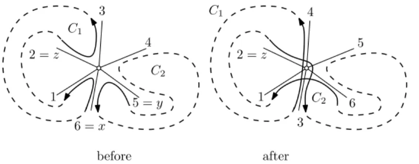
1 3 4 5 6 C1 C2 before after C1 C2 2 = z 5 = y 6 = x 1 3 4 2 = z
Figure 6: Applying rule EatSmall modifies the port number assignment at the shown node so that cycle C1 becomes shorter and C2 longer.
The next important lemma implies that a witness cycle can be found by repeatedly applying Merge3 and EatSmall.
Lemma 3. Let −→K be a two-way connected spanning subgraph of G such that all nodes in G are RH-traversable in −→K. Consider the set of RH-cycles generated by some port numbering of its nodes, with C∗
being the largest cycle according to some ordering γ. If neither Merge3 nor EatSmall can be applied to the nodes of C∗ then C∗ is a witness cycle.
Proof. Suppose, by contradiction, that C∗ does not span all the nodes in G. Let V′be the set of nodes of G
not traversed by C∗. Since−→K is two-way connected there exist two nodes u, v ∈ G, such that v belongs to
C∗and u ∈ V′, and the directed edges (u, v) and (v, u) belong to−→K. Edges (u, v) and (v, u) cannot belong
to different cycles of−→K because Merge3 would be applicable. Hence, (u, v) and (v, u) must both belong to the same cycle C′. However, (u, v) and (v, u) cannot be consecutive edges of C′ because this would imply
dv = 1 which is not the case, since v also belongs to C∗. Hence, C′ must visit v at least twice. However,
since C∗is the largest cycle we have γ(C′) < γ(C∗) and the conditions of applicability of rule EatSmall are
satisfied with C1= C′ and C2= C∗. This is a contradiction, proving the claim of the lemma.
3. Three-layer partition
The three-layer partition is a new, fast graph decomposition method that we shall use to efficiently construct periodic tours, both for oblivious agents in Section 4 and bounded-memory agents in Section 6. It is defined as follows.
For any set X of nodes in a graph G, the neighborhood of X (denoted by NG(X)) is the set of neighbors
of X in G, excluding nodes belonging to X. For any node v in G and subgraph T of G, we say that v is
saturated in T if v and all edges incident to v in G are also present in T .
Definition 2. A three-layer partition of a simple, connected, undirected graph G = (V, E) is a 4-tuple (X, Y, Z, TB) such that:
• The three sets X, Y , and Z form a partition of V . • Y = NG(X) and Z = NG(Y ) \ X.
• TB is a connected, cycle-free subgraph of G (i.e., a tree) with node set X ∪ Y in which all nodes from X are saturated.
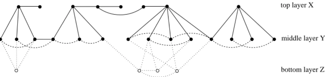
See Figure 7 for an example. We call X the top layer, Y the middle layer, and Z the bottom layer of the partition. Any edge of G between two nodes in Y is called horizontal, and the tree TB is called a backbone tree of G. Note that a backbone tree is not the same thing as a spanning tree (in particular, it does not
contain any node from the bottom layer Z); however, backbone trees will help us to find certain useful spanning trees later on.
middle layer Y
bottom layer Z top layer X
Figure 7: A three-layer partition. Solid lines and black nodes belong to the backbone tree TB. Dashed lines represent horizontal edges outside TB. Dotted lines represent edges that are incident to nodes from Z.
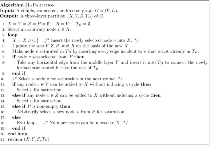
We now present a fast algorithm named 3L-Partition for constructing a three-layer partition with backbone tree TB of any given graph G = (V, E). The pseudocode is given in Figure 8. During execution,
the nodes in V are dynamically partitioned into sets X, Y, Z, P , and R with temporary contents, where: • X is the set of nodes currently saturated in TB.
• Y = NG(X) contains all nodes at distance 1 from X.
• Z = NG(Y ) \ X contains all nodes at distance 2 from X.
• P = NG(Z) \ Y contains all nodes at distance 3 from X.
• R = V \ (X ∪ Y ∪ Z ∪ P ) contains all remaining nodes from V .
(Thus, the contents of sets Y, Z, P , and R strictly depend on the current contents of X.) Initially, all nodes belong to R and the backbone tree TBis empty. Each iteration of the main loop (called a round ) makes one
node v saturated in TB by moving it to X and inserting the corresponding edges into TB. The algorithm
terminates when no more nodes can be saturated, i.e., can be added to X without inducing a cycle.
Algorithm 3L-Partition
Input: A simple, connected, undirected graph G = (V, E). Output: A three-layer partition (X, Y, Z, TB) of G.
1: X = Y = Z = P = ∅; R= V ; TB= ∅.
2: Select an arbitrary node v ∈ R. 3: loop
4: X= X ∪ {v} /* Insert the newly selected node v into X. */ 5: Update the sets Y, Z, P , and R on the basis of the new X.
6: Make node v saturated in TB by inserting every edge incident to v that is not already in TB.
7: if node v was selected from P then
8: Take any horizontal edge from the middle layer Y and insert it into TB to connect the newly
formed star rooted in v to the rest of TB.
9: end if
10: /* Select a node v for saturation in the next round. */
11: if any node v ∈ Y can be added to X without inducing a cycle then 12: Select v for saturation.
13: else if any node v ∈ Z can be added to X without inducing a cycle then 14: Select v for saturation.
15: else if P is non-empty then
16: Arbitrarily select a new node v from P for saturation. 17: else
18: Exit loop. /* No more nodes can be moved to X. */ 19: end if
20: end loop
21: return (X, Y, Z, TB)
Figure 8: Algorithm 3L-Partition.
Theorem 1. Algorithm 3L-Partition computes a three-layer partition of any simple, connected, undirected
graph G.
Proof. We shall show that the algorithm outputs a three-layer partition of G with a distinguished backbone
tree TB. We use the following invariant: At the end of each round, nodes in X and Y are spanned by a
partial backbone tree TB and a new node v is selected for saturation in the next round.
At the end of the first round, the invariant is satisfied because X consists of a single node whose neighbors in G form Y (step 5) and all edges incident to it belong to TB (step 6). Now assume that the invariant is
satisfied at the beginning of any round i > 1. When the newly selected node v is inserted into X (step 4), the contents of all other sets are updated (step 5). By definition, v is always selected in such a way that
a b c d z t u v x y a b c d z t u v x y a b c d z t u v x y a b c d z t u v x y a u z c b t v d x y e e e e e a b c d z t u v x y e (a) (b) (c) (d) (e) (-) X Y Z P R X Y Z P R all nodes belong to R here
Figure 9: An example of running Algorithm 3L-Partition. The input is the graph shown in (-), and (a)–(e) present the configuration in each round after a new node has been saturated and the sets X, Y, Z, P, R as well as the backbone tree TB have been updated. In (a)–(e), the current contents of each set X, Y, Z, P, R are displayed at different horizontal levels, and solid lines and black nodes belong to the backbone tree TB. The saturated nodes are a, b, c, d, and e, chosen from different sets Y, Z, and P .
adding all edges incident to v will not create a cycle in TB. If v was chosen from Y (this happens only
when v has no horizontal incident edges), v is already connected to TB so all edges incident to v (added in
step 6) will be connected to the rest of TB, too. Alternatively, if v comes from Z (this happens when all
nodes in Y have horizontal edges outside of TB) and v has exactly one neighbor w ∈ Y , then as soon as all
edges incident to v are inserted, the new part of TB gets connected to the old one via node w. Finally, if v
was selected from P (this happens when all nodes in Y have horizontal edges outside of TB and each node
in Z has at least two neighbors in Y ) then all edges incident to v are inserted into TB. Note that when v
was moved to X, all its neighbors in Z were moved to Y , forming at least one new horizontal edge in Y (formerly this edge lay across sets Y and Z). We use this new horizontal edge to connect a newly formed star with the remaining part of TB. The algorithm exits its main loop when it attempts to select a new node
for saturation from an empty set P , meaning that all nodes from V are already distributed among X, Y, Z, and in accordance with our invariant, this means that the backbone tree TB is completed.
Figure 9 illustrates the execution of Algorithm 3L-Partition.
The next two lemmas summarize some properties of Algorithm 3L-Partition that will be used later in the paper.
Lemma 4. The three-layer partition output by Algorithm 3L-Partition satisfies the following: 1. Each node y ∈ Y has an incident horizontal edge not belonging to TB.
2. Each node z ∈ Z has at least two neighbors in Y .
Proof. To prove property 1, assume by contradiction that there exists a node y ∈ Y with no horizontal edges
remaining edges incident to y. Indeed, since all such edges led only to nodes in Z before y was saturated, their insertion does not create any cycles. Thus, property 1 holds.
Next, assume there is a node z in Z with at most one incident edge leading to layer Y . Then, we can also saturate z since all edges incident to z form a star that shares at most one node with TB. Thus, no
cycle is created, which proves property 2.
Lemma 5. Algorithm 3L-Partition can be implemented to run in O(|E|) time.
Proof. Below, we say that any node of G is colored red if it has already been tested for saturation (regardless
of whether or not it was finally included in X), and green otherwise. All nodes are initially colored green and put in the set R. During the execution of steps 10–19 of 3L-Partition, a green node v is selected for saturation from one of the sets Y, Z, and P (in that order). Depending on which sets that v and its neighbors belong to, v either passes or fails the ensuing saturation test:
• If v ∈ Y then v may be saturated if none of its neighbors belongs to Y . • If v ∈ Z then v may be saturated if only one neighbor of v belongs to Y . • If v ∈ P then v may always be saturated.
If v passes the test then it will be saturated in the next iteration and promoted to X; on the other hand, if v fails the test, this means that saturating v would create a cycle in TB because of some edges already
present in TB. In both cases, the algorithm will never need to consider v for saturation again, and v can
be safely colored red. This shows that each node needs to be considered for saturation by steps 10–19 only once. The saturation test takes d(v) steps, i.e. O(|E|) time for all vertices.
Moreover, every (green or red) neighbor of a node v that is subjected to the above saturation test may be promoted to a higher ranking set among Y, Z, P and R depending on the result of the saturation test for v. This happens in the step of updating these sets (Step 5). Also in the same step, neighbors of newly promoted vertices may also be promoted, and this process continues until every vertex is listed correctly, as a result of promotions. However, note that vertices which are already in the backbone tree or have the same ranking with their newly promoted neighbor, will not be promoted by definition. This implies that not every vertex at distance two or three of a newly saturated vertex is needed to be checked for update.
Under these observations, it is preferable to amortize the number of checks/updates with the edges of the graph. Each edge can participate in promotional checks whenever one of its two vertices is involved. If each of the two endvertices reaches its highest possible ranking, the edge also stops participating in any promotional check. Note that each vertex can be checked for promotion more than once, but always via a different edge. Given that every vertex can be checked/promoted at most three times, this implies that the number of checks/updates per edge is a constant factor, and thus the overall cost of the updating step is also O(|E|).
Therefore, the complexity of the algorithm 3L-partition remains in O(|E|).
The three-layer partition method is employed in Section 4 and Section 6. We believe that this method may be of use for other problems as well in the future such as designing spanning trees with special properties, connected dominating sets, etc.
4. Efficient periodic graph traversal by an oblivious agent
The main result of this section is an algorithm named FindWitnessCycle that constructs a short witness cycle for any given graph G. By the remarks in Sections 2.2 and 2.3, this consequently solves the problem of periodic graph traversal by an oblivious agent.
According to Lemma 3, it is sufficient to construct a spanning subgraph −→K of G which is two-way connected such that each node of G is RH-traversable in −→K. We first consider a restricted case of a terse
set of RH-cycles in Section 4.1, for which it is possible to construct a spanning tree of G with no saturated
of arbitrary graphs considered in Section 4.2, we need a more involved argument, leading to a witness cycle of size ≤ (4 +13)n.
4.1. Terse set of RH-cycles
Suppose G is a graph that has a spanning tree T with no saturated nodes, i.e., for every node v, G contains some edge incident to v which does not belong to T . Here, we present an algorithm named TerseCycles that finds a very short witness cycle for this type of graphs.
Algorithm TerseCycles is listed in Figure 10. The idea is to first construct a spanning subgraph−→K of−→G that consists of RH-traversable nodes. For this purpose, TerseCycles takes the edges of a spanning tree T without saturated nodes as two-way edges in−→K, inserts some extra one-way edges, and then runs a procedure named RestoreParity, outlined in Figure 11, to make sure that the number of one-way edges in−→K incident to each node is always even. Procedure RestoreParity visits each node v of the tree T in bottom-up order and counts all one-way edges incident to v; if this number is odd, the two-way edge leading to the parent is reduced to a one-way edge (whose direction is unspecified at this point in time). Note that the cumulative degree of the root must be even since the cumulative degree of all nodes before restoring parity is even. At the conclusion of RestoreParity we remove temporarily from −→K all two-way edges. All one-way edges forming a connected component are arranged to form a single cycle. Now all these cycles are merged into a single witness cycle by adding a minimal number of previously removed two-way edges.
Algorithm TerseCycles
Input: A graph G that admits a spanning tree with no saturated nodes. Output: A witness cycle for G.
1: Let T be a spanning tree of G with no saturated nodes.
2: Construct−→K by replacing each edge {u, v} in T by two directed edges (u, v) and (v, u). 3: For each node v ∈ G, add to−→K a one-way edge incident to v and belonging to G \ T . 4: Root T arbitrarily.
5: RestoreParity(−→K , T, root(T ))
6: Remove temporarily from−→K all two-way edges.
7: Take any port numbering as in Lemma 2 and produce a set C of RH-cycles induced by it.
8: For any node v visited by two cycles entering v via ports i and j, swap i and j forming a single cycle. 9: Restore connectivity in−→K by adding back a minimal number of two-way edges.
10: Modify port numbers at each node to satisfy the construction in Lemma 2 while preserving the order of one-way edges.
11: return the cycle in C
Figure 10: Algorithm TerseCycles.
Lemma 6. After the completion of Algorithm TerseCycles, every node of −→K is RH-traversable. Proof. Every node is either saturated or has at least two one-way edges incident to it.
Corollary 2. For any graph G admitting a spanning tree T such that none of the nodes is saturated (i.e., G\ T spans all nodes of G), it is possible to construct a witness cycle of length at most 2n.
Proof. Observe that after the execution of Procedure TerseCycles, each node of v ∈−→K has an even (and non-zero) number of one-way edges incident to it. One can provide direction to all one-way edges and port numbering at each node v so that all edges outgoing from and incoming to v belong to the same cycle. This
Procedure RestoreParity
Input: A directed graph−→K (may be modified by the procedure), a tree T , and a node v ∈ T . Output: 0 or 1 (the parity for node v in−→K).
1: Pv = (number of one-way edges incident to v in
− →
K\ T ) (mod 2) 2: if v is not a leaf in T then
3: for each node cv∈ T that is a child of v do
4: Pv = (Pv+ RestoreP arity( − → K , T, cv)) (mod 2) 5: end for 6: end if 7: if Pv= 1 then
8: Reduce the two-way edge (v, parent(v)) to a one-way edge in−→K with unspecified direction. 9: end if
10: return Pv
Figure 11: Procedure RestoreParity.
is done in two steps. First, the initial port numbering and the direction of one-way edges are obtained via greedy selection of one-way edges to form cycles. Later, if there is a node v that belongs to two or more cycles (based on one-way edges), the cycles are merged at v via direct port number manipulation. When this stage is done, the set of nodes in−→K is partitioned into components, with all nodes in the same component belonging to the same cycle based on one-way edges. Also note that each component is at distance one from some other component, where the components are connected by at least one two-way edge (this is a consequence of the fact that each node has at least two one-way edges incident to it). The two-way edge is used to connect the components. By successively connecting pairs of components at distance one, we end up with a single component, i.e., a witness cycle spanning all the nodes. It is important to only add a minimal set of two-way edges enforcing connectivity to actually end up with a single cycle. Note that for each one-way edge introduced in−→K, a two-way edge from the spanning tree is reduced to a one-way edge during the restore parity process. This happens because one-way edges form a collection of stars and at least one endpoint of every one-way edge (in a star) is free. Thus, the number of all edges in the witness cycle is bounded by 2n.
By Corollary 2, Algorithm TerseCycles yields a small witness cycle for any graph that admits a spanning tree with no saturated nodes. This situation occurs for large, non-trivial classes of graphs, including two-connected graphs, graphs admitting two disjoint spanning trees, and many others. On the negative side, observe that in general, finding a spanning tree having no saturated nodes amounts to finding a Hamiltonian path, a problem known to be NP-hard even if restricted to 3-regular, planar graphs [6].
4.2. Construction of witness cycles in arbitrary graphs
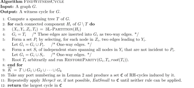
Given any graph G, Algorithm FindWitnessCycle in Figure 12 can be used to construct a witness cycle for G. The algorithm is based on the following approach. First compute a spanning tree T of G. Let Hi for i = 1, 2, . . . , k be the connected components of G \ T , having, respectively, ni nodes. For each such
component, run Algorithm 3L-Partition, obtaining three sets Xi, Yi, Zi and a backbone tree Ti. Use the
edges of Tias two-way edges in Gi, insert extra one-way edges incident to the nodes of sets Yi and Zi, and
apply the procedure RestoreParity. We shall explain below how to do this so that the total number of edges in all resulting Gi-graphs is smaller than (2 +13)n. Next, we let
− →
K be the union of T (where every edge of T is used both directions) with all the Gi-graphs, and take a port numbering that generates a set of
RH-cycles as in Lemma 2. Finally, we apply rules Merge3 and EatSmall to this set of cycles until neither rule can be applied. The set of cycles obtained will contain a witness cycle according to Lemma 3.
Algorithm FindWitnessCycle Input: A graph G.
Output: A witness cycle for G. 1: Compute a spanning tree T of G.
2: for each connected component Hi of G \ T do
3: (Xi, Yi, Zi, Ti) = 3L-Partition(Hi)
4: Gi= Ti /* These edges are inserted into Gi as two-way edges. */
5: Form a set Pi by selecting, for each node in Zi, two edges leading to Yi.
Let Gi = Gi∪ Pi. /* One-way edges. */
6: Form a set Si of independent stars spanning all nodes in Yi that are not incident to Pi.
Let Gi = Gi∪ Si. /* One-way edges. */
7: Root Ti arbitrarily and run RestoreParity(Gi, Ti, root(Ti)).
8: end for
9: −→K = T ∪ G1∪ G2∪ · · · ∪ Gk
10: Take any port numbering as in Lemma 2 and produce a set C of RH-cycles induced by it. 11: Repeatedly apply Merge3 or, if not possible, EatSmall to C until neither rule can be applied. 12: return the largest cycle in C
Figure 12: Algorithm FindWitnessCycle.
Theorem 2. For any n-node graph algorithm, FindWitnessCycle returns a witness cycle of size at most (4 +1
3)n − 4.
Proof. For each component Hi, we apply Algorithm 3L-Partition to obtain three sets Xi, Yi, Zi and a
backbone tree Ti. By Lemma 4, we can add one-way edges incident to the nodes in Yi as well as pairs of
one-way edges incident to the nodes in Zi and then apply Procedure RestoreParity to each Gi. Note
that when each star Si is constructed, we may do it in such a way that no path of length three or more is
created. Indeed, otherwise we could remove a middle edge of any path of length three and the set of spanned nodes would remain the same. Hence, Si is a forest of stars. Moreover, we can assume that only centers
of such stars can be incident to edges forming Pi,otherwise any edge leading to a leaf node incident to Pi
can be removed. Consequently, after termination of the “for” loop, each node of G is RH-traversable in−→K. Moreover, since−→K ⊇ T ,−→K is two-way connected, so the conditions of Lemma 3 are satisfied. Hence, at the end of the algorithm, C contains a witness cycle.
In order to bound the size of the witness cycle, we will bound the number of edges in−→K. First note that 2n − 2 edges originate from T (i.e., n − 1 two-way edges). Suppose that for each component Gi containing
ni nodes of G \ T , no one-way edges were added in lines 5 and 6, that is Pi= ∅ and Si= ∅. Hence, the call
to Procedure RestoreParity in line 7 did not modify Gi. In consequence, 2(ni− 1) edges were added for
Gi or 2(n1+ n2+ · · · + nk) − 2k in total. This value is maximized for k = 1, giving 2n − 2 edges added in
the “for” loop, and 4n − 4 total edges in−→K. The count remains the same if some Pi6= ∅ since exactly two
edges were added for each node of Zi in line 5.
Now suppose that Si6= ∅ in line 6, for some components Gi. For each endpoint v ∈ Yiof a star belonging
to Si and a one-way edge e added for v in Si in line 6, we check whether there is some other edge that was
reduced (from two-way to one-way) during the call to RestoreParity on line 7. This happens when v is not incident to a horizontal edge of the backbone tree Ti, since one of the edges incident to v will then
become a one-way edge. Thus, the addition of e is done at no extra cost, i.e., the total number of edges remains the same. However, when two endpoints of a horizontal edge are incident to two edges of Ti, only
one such edge will be amortized. Consider then a collection of one-way horizontal edges, belonging to the backbone tree Ti with edges of Si incident to both of their endpoints. The collection forms a forest. In
arbitrary leaf and amortize the edge of Si incident to it with the tree edge leading to the parent of the leaf.
Remove the leaf and the edge that leads to its parent from further consideration. Note that in this case, amortization is one to one. When this process is finished, each tree has been reduced to one edge. In other words, we have a collection of independent one-way horizontal edges belonging to the backbone tree. Note that each such edge is associated with two independent edges of Si. Clearly, the worst case happens when
the forest was formed by independent one-way edges. This implies that the number of such horizontal edges is not larger than ni
3.
Taking into consideration the maximal penalty that we have to pay for edges added in line 6 of the algorithm, the number of edges forming−→K is bounded by (4 + 1
3)n − 4.
Next, we analyze the algorithm’s time complexity.
Theorem 3. Algorithm FindWitnessCycle can be implemented so it runs in O(|E|) time.
Proof. In O(|E|) time we can find a spanning tree T of G and the connected components of G\T . By Lemma
5, for each connected component Gi having ni nodes and ei edges, Algorithm 3L-Partition terminates
in O(ei) time. The construction of sets Pi in line 5 and set Si in line 6 as well as the call to procedure
RestoreParity on line 7 are completed in O(ni) time. Altogether, the “for” loop terminates in O(|E|) time. The construction of−→K in line 9 and C in line 10 are done in time proportional to their sizes, i.e., O(n). We show now that line 11, where the rules Merge3 and EatSmall are repeatedly applied, may be per-formed within O(|E|) time. We chose any ordering γ of cycles and we attach to each edge a label corre-sponding to the cycle to which the edge belongs. Let C∗ be the largest cycle according to γ and v be any
node of C∗. We repeatedly apply rules Merge3 (resulting cycle obtaining rank of γ(C∗)) and EatSmall to
node v until no longer possible. Observe that, for each node v, this may be done in time proportional to the degree of node v in−→K, resulting in the overall cost of O(|E|). Each time, we traverse the edges of the cycle (or a part of the cycle) added to C∗and change their labels to γ(C∗). When neither Merge3 nor EatSmall is
applicable to v we proceed to node v′(the actual successor of v in C∗) and repeat the procedure of applying
rules Merge3 or EatSmall to v′. Each edge introduced in C∗ was relabeled exactly once, hence the overall
cost of relabeling process is in O(|E|). Although C∗ changes dynamically and some nodes may be traversed
many times we end up by traversing all nodes eventually in C∗. By Lemma 3, C∗ becomes a witness cycle
at the end of this process. Note that the complexity of each Merge3 and EatSmall operation is proportional to the number of edges added to C∗. By Theorem 2, the overall complexity of line 11 is O(|E|).
Finally, we provide a lower bound example for the FindWitnessCycle algorithm which demonstrates that the bound stated in Theorem 2 for our algorithm is tight, up to an additive constant.
Lemma 7. There exist graphs for which the FindWitnessCycle algorithm may produce a witness cycle
of size (4 +1 3)n − 7.
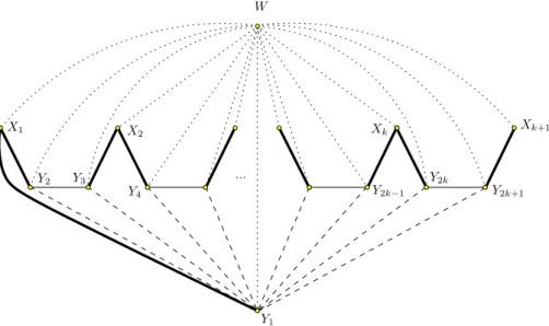
Proof. Consider the graph in Figure 13.
The main part of the graph containing n = (3k+1) nodes consists of k copies of four nodes XiY2iY2i+1Xi+1,
for i = 1, 2, . . . , k, where the last node of each but the last copy is identified with the first node of the next copy (see Figure 13). Moreover, an extra node Y1 is adjacent to each of the nodes Y2, Y3, . . . , Y2k+1, and
a node W is adjacent to all other nodes in the graph. Suppose that the star at node W is chosen by the algorithm as the spanning tree T , represented by the dotted edges in the picture. Algorithm 3L-Partition locates nodes X1, X2, . . . , Xk in set X and the nodes Y1, Y2, . . . , Y2k+1 in set Y (set Z is empty). Suppose
that the backbone tree is the path Y1X1. . . Xk+1 - represented by the solid edges in Figure 13. Since the
algorithm adds one horizontal edge for each node from class Y , all edges incident to Y1 are added to the
structures. It is easy to see that the parity restoring procedure will chose the edges YiYi+1 as the one-way
edges of the structure. In consequence, only 2k dashed edges and k thin solid edges in Figure 13 are chosen as one-way edges; all other edges (i.e., 3k + 2 dotted edges and 2k + 1 bold solid edges) are taken as two-way edges. This results in a witness cycle of size 13k + 6, i.e., containing (4 +13)n − 7 edges.
Y1 Y2 Y3 Y4 Y2k−1 Y2k Y2k+1 X1 X2 Xk+1 Xk W ...
Figure 13: Example of a graph for which our algorithm gives a witness cycle of size not smaller than (4 +1 3)n − 7.
5. A lower bound for oblivious agents
The previous section showed that for any n-node graph, we can construct a witness cycle of length at most (4 +1
3)n − 4. In this section, we complement this result with a non-trivial lower bound of 2.8n − 2.
Theorem 4. For any non-negative integers n, k, and l such that n = 5k + l and l < 5, there exists an n-node graph for which any witness cycle is of length 14k + 2l − 2.
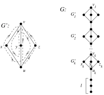
Proof. First consider a single diamond graph G′with 5 nodes, defined on the left side of Figure 14. W.l.o.g.,
assume that the agent starts its traversal through the edge (v, x). By the structure of G′, the agent then
traverses the edge (x, u). Again, w.l.o.g., suppose the successor of (x, u) is the edge (u, y). Then there is only one feasible successor of (y, v), namely (v, z), because the other two edges either violate RH-traversability ((v, y)) or leave node z unvisited ((v, x)). Next, the only possible successor of (z, u) is (u, x) because (u, y) has already been traversed with a different predecessor and (u, z) violates RH-traversability. Similarly, the successor of (x, v) must be (v, y) and the successor of (y, u) must be (u, z). Therefore, each edge of G′ must
be used in both directions, and the witness cycle has length 12 = 2.4n.
Next, consider the graph G having n nodes and consisting of a chain of k diamond graphs and path of lnodes attached to node uk, as shown on the right side of Figure 14. Note that G contains 7k + (l − 1) edges.
Assume that the agent start the graph traversal at node v1. From the fact that each edge in the witness
cycle is traversed at most twice (one time in each direction), it follows that when returning to ui−1 from vi,
all nodes in Gi (as well as in all Gj for j > i) must have been visited. From RH-traversability, it follows
that the successor of (ui−1, vi) cannot be the same (in reverse direction) as the predecessor of (vi, ui−1), and
similarly the successor of (vi, ui−1) cannot be the same as the predecessor of (ui−1, vi). In turn, this means
that analogous arguments as used above for the graph G′ also apply to every Gi. Therefore, all edges of G
must be traversed in both directions.
Selecting l = 0 in Theorem 4 gives n = 5k, and we obtain the lower bound 14k − 2 = 2.8n − 2 on the period length for oblivious agents.
6. Periodic graph traversal by an agent with constant memory
In this section, we focus on algorithms for periodic graph traversal by agents with constant memory. The main idea of the periodic graph traversal mechanism proposed in [8], and further developed in [7], is to visit
xk yk zk k v k u ... v 1
G:
1 k G’ G’ 2 l G’G’:
y u v x zFigure 14: The diamond graph G′and the chain of diamond graphs used to prove the lower bound in Theorem 4. The witness cycle for G′ shown on the left is hv, x, u, y, v, z, u, x, v, y, u, z, vi with length 12.
all nodes in the graph while traversing along an Euler tour of a (in [7], particularly chosen) spanning tree. In [8], an arbitrary spanning tree T of G is rooted at any leaf, and the port numbers assigned so that at each non-root node v, port 1 is assigned to the port leading to the parent of v while ports {2, . . . , i + 1} are assigned to the children of v in T and ports {i + 2, . . . , dv} to the remaining ports. Then, after entering
node v via port 1, the agent recursively visits all subtrees accessible from v via ports 2, . . . , i + 1, where i is the number of children of v. When the agent returns from the last (ith) child it either: (1) returns to its parent via port 1, when i + 1 is also the degree of v (i.e., v is saturated in T ); or (2) it attempts to visit another child of v by traversing the edge e associated with port i + 2. In case (2), the agent learns at the other end of e that the port number is different from 1, i.e., that this node is not a child of v in the spanning tree T , and uses its constant memory to immediately backtrack via the same edge (first return to v and then directly to the parent of v), and then continues the tree traversal process. In these circumstances, the edge e is called a penalty edge since e does not belong to the spanning tree and an extra cost has to be charged for traversing it. Since the spanning tree has n − 1 edges, and at each node the agent can be forced to traverse a penalty edge, the number of steps performed by the agent (equal to the length of the periodic tour) may be as large as 4n − 2 (n − 1 edges of the spanning tree and n penalty edges, where each edge is traversed in both directions). The main result of [7] is the efficient construction of a specific spanning tree supported by a more advanced visiting mechanism stored in the agent’s memory. They showed that the agent is able to avoid penalties at a fraction of at least 18nnodes. This in turn gave the length of the periodic tour not larger than 3.75n − 2.
In what follows, we show a new construction of the spanning tree, based on the earlier three-layer partition. This, supported by a new labeling mechanism together with slightly increased memory of the agent, allows us to avoid penalties at 1
4nnodes, resulting in a periodic tour of length ≤ 3.5n. In the new
scheme, shortcuts are created by performing “port swap operations”, where some leaves in the spanning tree are connected to their parents via port 2 (in [7], this port is always assumed to be 1). The rationale behind this modification is to treat edges towards certain leaves as penalty edges (rather than the regular tree edges) and in turn to avoid visits beyond these leaves, i.e., to avoid unnecessary examination of certain penalty edges.
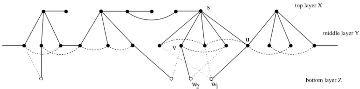
w2 w1 bottom layer Z middle layer Y top layer X s v u
Figure 15: Fragment of the spanning tree with the root located to the right of w1and w2.
6.1. The construction
Recall that the nodes of the input graph can be partitioned into three layers X, Y , and Z, where all nodes in X and Y are spanned by a backbone tree; see Section 3. The spanning tree T is obtained from the backbone tree by connecting every node in Z to one of its neighbors in Y. Also recall that every node v ∈ X is saturated, i.e., all edges incident to v in G also belong to the spanning tree. Every node in Y that lies on a path in T between two nodes in X is called a bonding node. The remaining nodes in Y are called local.
Initial port labeling:
When the spanning tree T is formed, we pick one of its leaves as the root r where the two ports located on the tree edge incident to r are set to 1. Initially, for any node v the port leading to the parent is set to 1 and ports leading to the i children of v are set to 2, . . . , i + 1 in such a way that the subtree of v rooted in child j is at least as large as the subtree rooted in child j′ for all 2 ≤ j < j′ ≤ i + 1. All other ports are
set arbitrarily using distinct values from the range i + 2, . . . , dv, where dv is the degree of v. Port swap operations:
Now, we modify allocation of ports at certain leaves of the spanning tree located in Z. In particular, we change labels at all children having no other leaf-siblings in T of bonding nodes (see, e.g., node w1 in
Figure 15), as well as in single children of local nodes, but only if the local node is the last child of a node in X that has children on its own (see, e.g., node w2in Figure 15).
Every leaf w located in layer Z has an incident edge e outside of T that leads to some node v in Y by Lemma 4 (property 2). When swapping port numbers at some leaf w, we set the port number on the tree edge leading to the parent of w to 2. We call such an edge a sham penalty edge since it appears to be a penalty edge but in fact connects w to its parent in the spanning tree T . We also set the port number on the lower end of e to 1. All other port numbers at w (if there are more incident edges to w) are set arbitrarily. After the port swap operation at w is accomplished we also have to ensure that the edge e will never be examined by the agent, otherwise it would be wrongly interpreted as a legal tree edge, where v would be recognized as the parent of w. In order to avoid this problem we also set ports at v with greater care. Note that v has also an incident horizontal edge e′ outside of T (property 1 of the three-layer partition). Assume
that the node v has i children in T. Thus, if we set to i + 2 the port on e′ (recall that port 1 leads to the
parent of v and ports 2, . . . , i + 1 lead to its children) the port on e will have value larger than i + 2 and ewill never be accessed by the agent. Finally, note that the agent may wake up in the node with a sham penalty edge incident to it. For this reason, we introduce an extra state to the finite state automaton A governing moves of the agent in [7] to form a new automaton A+. While being in the wake up state the
agent moves across the edge accessible via port 1 in order to start regular performance (specified in [7]) in a node that is not incident to the lower end of a sham penalty edge.
Lemma 8. The new port labeling provides a mechanism to visit all nodes in the graph in a periodic manner
middle layer Y
...
bottom layer Z (a) (b) (c) (d) top layer X v u wFigure 16: Cases (a), (b), (c), and (d) of the local amortization argument used in the proof of Theorem 5.
Proof. It suffices to prove that no difficulty arises at nodes with numbers affected by the modified labeling
scheme.
Case C1: First consider the case when the port numbers are swapped at some node w1 which is a single
child in Z of a bonding node u (see Figure 15). When during traversal the agent returns from the subtree rooted in a child of u accessible via port i − 1, it enters via port i the edge leading to w1. This edge is
interpreted as a penalty edge and the agent after visiting w1 immediately returns to u and then it goes
with no further action to the parent of u. Note that if the labeling was not changed the agent would act similarly; however, it would additionally examine a penalty edge located at w1. Thus, thanks to the new
labeling scheme we save one penalty at the node w1.
Case C2: Next, consider the case when the port numbers are swapped at a single child w2of a local node
v such that v has no siblings different from leaves to its right (accessible via larger ports), see Figure 15. Assume that s is the (saturated) parent of v and port i at v leads to w2.When during traversal the agent
returns from the subtree rooted in a child of v accessible via port i − 1, it enters via port i the edge leading to w2.When it learns that the port label at w2 is different from 1, it interprets the sham penalty edge linking
v and w2 as the penalty edge. The agent immediately returns to v while switching to the leaf recognition
state [7] (v would be interpreted as the first leaf of s). This means that all remaining leaves accessible from s(if any) will be visited at no extra charge, i.e., without paying penalty at them. Thus, the agent does not miss the node w2and it also saves penalty at w2and possibly at all leaves that are siblings of v.
6.2. Analysis
Theorem 5. For any undirected graph G with n nodes, it is possible to compute a port labeling such that
an agent equipped with a finite state automaton A+ can visit all nodes in G in a periodic manner with a tour length that is no longer than 3.5n − 2.
Proof. The main line of the proof explores the fact that the fraction of nodes at which the agent manages
to save on penalties is at least 1
4. The proof is split into global and local amortization arguments.
• Global amortization [saturated nodes amortize all bonding nodes and single children of saturated nodes]
Note that in a three-layer partition with k saturated nodes, there are at most 2k − 2 bonding nodes since introducing a new saturated node implies the creation of at most two bonding nodes. Also note that there are at most k single leaves (with no siblings) that are children of saturated nodes. In the global amortization argument, we assume that at these nodes, i.e., all bonding nodes and all single leaves of saturated nodes, in the worst case the agent always pays penalty (examines the penalty edge). Fortunately, all of these ≤ 3k − 2 nodes (2k − 2 bonding nodes and k single leaves of saturated nodes) can be amortized by k saturated nodes. Thus, as required, the fraction of nodes where the agent does not pay penalty is 1