HAL Id: hal-01146187
https://hal.inria.fr/hal-01146187
Submitted on 20 Jul 2015
HAL is a multi-disciplinary open access
archive for the deposit and dissemination of
sci-entific research documents, whether they are
pub-lished or not. The documents may come from
teaching and research institutions in France or
abroad, or from public or private research centers.
L’archive ouverte pluridisciplinaire HAL, est
destinée au dépôt et à la diffusion de documents
scientifiques de niveau recherche, publiés ou non,
émanant des établissements d’enseignement et de
recherche français ou étrangers, des laboratoires
publics ou privés.
Maximum Entropy Semi-Supervised Inverse
Reinforcement Learning
Julien Audiffren, Michal Valko, Alessandro Lazaric, Mohammad Ghavamzadeh
To cite this version:
Julien Audiffren, Michal Valko, Alessandro Lazaric, Mohammad Ghavamzadeh. Maximum Entropy
Semi-Supervised Inverse Reinforcement Learning. International Joint Conference on Artificial
Intelli-gence, Jul 2015, Bueons Aires, Argentina. �hal-01146187�
Maximum Entropy Semi-Supervised Inverse Reinforcement Learning
Julien Audiffren
Michal Valko
Alessandro Lazaric
Mohammad Ghavamzadeh
CMLA UMR 8536
SequeL team
SequeL team
Adobe Research &
ENS Cachan
INRIA Lille
INRIA Lille
INRIA Lille
Abstract
A popular approach to apprenticeship learning (AL) is to formulate it as an inverse reinforce-ment learning (IRL) problem. The MaxEnt-IRL al-gorithm successfully integrates the maximum en-tropy principle into IRL and unlike its predecessors, it resolves the ambiguity arising from the fact that a possibly large number of policies could match the expert’s behavior. In this paper, we study an AL setting in which in addition to the expert’s tra-jectories, a number of unsupervised trajectories is available. We introduce MESSI, a novel algorithm that combines MaxEnt-IRL with principles com-ing from semi-supervised learncom-ing. In particular, MESSI integrates the unsupervised data into the MaxEnt-IRL framework using a pairwise penalty on trajectories. Empirical results in a highway driv-ing and grid-world problems indicate that MESSI is able to take advantage of the unsupervised trajecto-ries and improve the performance of MaxEnt-IRL.
1
Introduction
The most common approach to solve a sequential decision-making problem is to formulate it as a Markov decision pro-cess (MDP) and then use dynamic programming or reinforce-ment learning to compute a near-optimal policy. This pro-cess requires the definition of a reward function such that the policy obtained by optimizing the resulting MDP pro-duces the desired behavior. However, in many applications such as driving or playing tennis, it is required to take into account different desirable factors and it might be difficult to define an explicit reward function that accurately speci-fies the trade-off. It is often easier and more natural to learn how to perform such tasks by imitating an expert’s demon-stration. The task of learning from an expert is called
ap-prenticeship learning(AL). An effective and relatively novel
approach to apprenticeship learning is to formulate it as an
inverse reinforcement learning(IRL) problem [Ng and
Rus-sell, 2000]. The basic idea is to assume that the expert is optimizing an MDP whose reward function is unknown and to derive an algorithm for learning the policy demonstrated by the expert. This approach has been shown to be effec-tive in learning non-trivial tasks such as inverted helicopter
flight control [Ng et al., 2004], ball-in-a-cup [Boularias et
al., 2011], and driving on a highway [Abbeel and Ng, 2004;
Levine et al., 2011]. In the IRL approach to AL, we assume that several trajectories generated by an expert are available and the unknown reward function optimized by the expert can be specified as a linear combination of a set of state features. For each trajectory, we define its feature count as the sum of the values of each feature across the states traversed by the trajectory. The expected feature count is computed as the av-erage of the feature counts of all available expert trajectories, thus implicitly encoding the behavior and preference of the expert. The goal is to find policies whose expected feature
counts match that of the expert.1The early method of Abbeel
and Ng [2004] finds such policies (reward functions) using an iterative max-margin algorithm. Its major disadvantage is that the problem is ill-defined since a large number of policies can possibly satisfy such matching condition. In this paper, we build on the work of Ziebart et al. [2008] who proposed a method based on the maximum entropy (MaxEnt) principle to resolve this ambiguity.
In many applications, in addition to the expert’s trajecto-ries, we may have access to a large number of trajectories that are not necessarily performed by an expert. For example, in learning to drive, we may ask an expert driver to demon-strate a few trajectories and use them in an AL algorithm to mimic her behavior. At the same time, we may record tra-jectories from many other drivers for which we cannot as-sess their quality (unless we ask an expert driver to evaluate them) and that may or may not demonstrate an expert-level behavior. We will refer to them as unsupervised trajectories and to the task of learning with them as semi-supervised
ap-prenticeship learning [Valko et al., 2012]. However, unlike in
classification, we do not regard the unsupervised trajectories as being a mixture of expert and non-expert classes. This is because the unsupervised trajectories might have been gener-ated by the expert themselves, by another expert(s), by near-expert agents, by agents maximizing different reward func-tions, or simply they can be some noisy data. The objective of IRL is to find the reward function maximized by the expert, and thus, semi-supervised apprenticeship learning is not a di-1More precisely, the goal is to find reward functions such that the
expected feature count of the (near)-optimal policies of the resulting MDPs match that of the expert.
rect application of semi-supervised classification.2Similar to many IRL algorithms that draw inspiration from supervised learning, in this paper, we build on semi-supervised learning (SSL, Chapelle et al. 2006) tools to derive a novel version of MaxEnt-IRL that takes advantage of unsupervised trajec-tories to improve the performance. In our first attempt, we had proposed [Valko et al., 2012] a semi-supervised appren-ticeship learning paradigm, called SSIRL, that combines the IRL approach of Abbeel and Ng [2004] with semi-supervised SVMs, and showed how it could take advantage of the unsu-pervised data and perform better and more efficiently (with less number of iterations, and thus, solving less MDPs) than the original algorithm. Nonetheless, as we will discuss in Sect. 3, SSIRL still suffers from the ill-defined nature of this class of IRL methods and the fact that all the policies (reward functions) generated over the iterations are labeled as “bad”. This creates more problems in the SSL case than in the origi-nal setting. In fact, SSIRL relies on a cluster assumption that assumes the good and bad trajectories are well-separated in some feature space, but this never holds as new policies are generated and labeled as “bad”. Finally, SSIRL is rather a proof of concept than an actual algorithm, as it does not have a stopping criterion, and over iterations the performance al-ways reverts back to the performance of the basic algorithm by Abbeel and Ng [2004]. In Sec. 3, we address these prob-lems by combining MaxEnt-IRL of Ziebart et al. [2008] with SSL. We show how unsupervised trajectories can be inte-grated into the MaxEnt-IRL framework in a way such that the resulting algorithm, MESSI (MaxEnt Semi-Supervised IRL), performs better than MaxEnt-IRL. In Sec. 4, we empirically show this improvement in the highway driving problem of Syed et al. [2008]. Additional experiments are available in the appendix.
2
Background and Notations
A Markov decision process (MDP) is a tuple hS, A, r, pi, where S is the state space, A is the action space, r : S → R is the state-reward function, and p : S × A → ∆(S) is
the dynamics, such that p(s0
|s, a) is the probability of
reach-ing state s0 by taking action a in state s. We also denote by
π : S → ∆(A) a (stochastic) policy, mapping states to
dis-tributions over actions. We assume that the reward function can be expressed as a linear combination of state-features.
Formally, let f : S → Rd be a mapping from the state
space to a d-dimensional feature space and let fi denote the
i-th component of the vector f, then we assume that the
re-ward function is fully characterized by a vector θ ∈ Rd
such that for any s ∈ S, rθ(s) = θTf(s). A trajectory
ζ = (s1, a1, s2, . . . , aT −1, sT) is a sequence of states and
actions,3whose cumulative reward is
¯ rθ(ζ) = T X t=1 rθ(st) = T X t=1 θTf(s t) = θT T X t=1 f(st) = θTfζ, (1)
2If that was the case, then the AL problem would reduce to a
clas-sical supervised learning problem upon revealing the expert/non-expert labels of the additional trajectories, which is not the case.
3In practice, MaxEnt-IRL and our extension do not require a
tra-jectory to include actions and only states are needed.
where fζ is the feature count of ζ that measures the
cumu-lative relevance of each component fi of the feature vector
along the states traversed by ζ.4In AL, we assume that only
ltrajectories Σ∗ = {ζ∗
i} l
i=1 are demonstrated by the expert
and we define the corresponding expected feature count as
f∗ = 1
l
Pl
i=1fζ∗
i. The expected feature count f
∗
summa-rizes the behavior of the expert since it defines which features are often “visited” by the expert, thus implicitly revealing her preferences, even without an explicit definition of the reward. This evidence is at the basis of the expected feature-count matching idea (see e.g., Abbeel and Ng 2004), which defines the objective of AL as finding a policy π whose
correspond-ing distribution Pπover trajectories is such that the expected
feature count of π matches the expert’s, i.e., X
ζ
Pπ(ζ)fζ = f∗, (2)
where the summation is taken over all possible trajectories. Ziebart et al. [2008] pointed out there is a large number of policies that satisfy the matching condition in Eq. 2 and intro-duced a method to resolve this ambiguity and to discriminate between different policies π based on the actual reward they accumulate, so that the higher the reward the higher the prob-ability. Building on the maximum entropy principle, Ziebart et al. [2008] move from the space of policies to the space of trajectories and define the probability of a trajectory ζ in an MDP characterized by a reward function defined by θ as
P(ζ|θ) ≈exp(θ Tf ζ) Z(θ) T Y t=1 p(st+1|st, at),
where Z(θ) is a normalization constant and the approxima-tion comes from the assumpapproxima-tion that the transiapproxima-tion random-ness has a limited effect on behavior. The policy π induced by the reward θ is
π(a|s; θ) = X
ζ∈Σs,a
P(ζ|θ), (3)
where Σs,adenotes the set of trajectories for which action a is
taken in state s. MaxEnt-IRL searches for the reward vector θ that maximizes the log-likelihood of θ of a given set of expert
trajectories Σ∗= {ζ∗ i}li=1, i.e., θ∗= arg max θ L(θ|Σ ∗) = arg max θ l X i=1 log P (ζ∗ i|θ). (4)
The resulting reward is such that the corresponding
distribu-tion over trajectories, PζP(ζ|θ
∗
)fζ, matches the expected
feature count f∗, and at the same time, it strongly penalizes
trajectories (and implicitly policies) that do not achieve as much reward as the expert.
3
Maximum Entropy Semi-Supervised
Inverse Reinforcement Learning
The main objective of semi-supervised learning (SSL, Chapelle et al. 2006) is to bias the learning toward models that assign similar outputs to intrinsically similar data.
Sim-4Note that if f : S → {0, 1}, then fi
ζreduces to a counter of the
ilarity is commonly formalized in SSL as manifold, cluster, or other smoothness assumptions. Previously, we had inte-grated [Valko et al., 2012] a semi-supervised regularizer into the SVM-like structure of the feature matching algorithm of Abbeel and Ng [2004] under an implicit clustering assump-tion. Although the integration is technically sound, the SSL hypothesis of the existence of clusters grouping trajectories with different performance is not robust w.r.t. the learning al-gorithm. In fact, even when assuming that expert and non-expert policies (used to generate part of the unsupervised tra-jectories) are actually clustered, newly generated policies are always labeled as “negative”, and as they become more and more similar to the expert’s policy, they will eventually cross the clusters and invalidate the SSL hypothesis. Let us stress that MaxEnt-IRL, which we build on, is also not a classical supervised method (e.g., classification) as it does not take as input a set of labeled trajectories (e.g., positive/negative). Un-like imitation learning, that can be directly framed as a classi-fication problem, IRL algorithms rely on supervised methods to solve a problem which is not supervised in its initial formu-lation. In our setting, there is no clear definition of “class” of trajectories that could be exploited by MaxEnt-IRL. Even if we knew that a unsupervised trajectory is not from the expert, we would not know how to explicitly use it in MaxEnt-IRL.
In this section, we propose an SSL solution to AL with unsupervised trajectories. To avoid the problems of the prior work, we do not reduce the problem to SSL classification. We modify maximum entropy framework to obtain an optimiza-tion problem that reflects the structural assumpoptimiza-tions of the geometry of the data. In our context, a similar, yet different approach is applied to MaxEnt-IRL that leads to constraining the probabilities of the trajectories to be locally consistent.
Pairwise Penalty and Similarity Function
We assume that the learner is provided with a set of expert
tra-jectories Σ∗=
{ζ∗
i}li=1and a set of unsupervised trajectories
e
Σ = {ζj}uj=1. We also assume that a function s is provided
to measure the similarity s(ζ, ζ0)between any pair of
trajec-tories (ζ, ζ0). We define the pairwise penalty R as
R(θ|Σ) = 1 2(l + u) X ζ,ζ0∈Σ s(ζ, ζ0) (θT(f ζ− fζ0))2, (5) where Σ = Σ∗∪ eΣ, and f
ζ and fζ0 are the feature counts for
trajectories ζ, ζ0
∈ Σ, and (θT
(fζ− fζ0))2= (¯rθ(ζ)− ¯rθ(ζ0))2,
is the difference in rewards accumulated by the two trajec-tories w.r.t. the reward vector θ. The purpose of the pairwise penalty is to penalize reward vectors θ that assign very
differ-ent rewards to similar trajectories (as measured by s(ζ, ζ0)).
In other words, the pairwise penalty acts as a regularizer which favors vectors that give similar rewards to similar tra-jectories. On the other hand, when two trajectories are very
different, s(ζ, ζ0)is very small, and θ is not constrained to
give them a similar reward.
In SSL, there are several ways to integrate a smoothness penalty R(θ) into the learning objective. In our case, we take inspiration from Erkan and Altun [2009] for the use of the pairwise penalty in MaxEnt, but then we add it to the dual
problem rather than to the primal, as adding the penalty to the dual would not be tractable. This corresponds to adding the penalty R(θ) to the MaxEnt-IRL optimization of Eq. 4 as
θ∗= argmax
θ (L(θ|Σ
∗)
− λR(θ|Σ)) , (6)
where λ is a parameter trading off between the log-likelihood of θ w.r.t. the expert’s trajectories and the coherence with the
similarity between the trajectories in Σe and Σ∗. This
modi-fication is motivated by the reduction of the number of pa-rameters: indeed, following the derivation in Erkan and
Al-tun [2009] would lead to a different algorithm with l2
addi-tional parameters, hence greatly increasing the computaaddi-tional complexity of the problem. As it is often the case in SSL, the choice of the similarity is critical to the success of learn-ing, since it encodes a prior on the characteristics two tra-jectories should share when they have similar performance, and it defines how unsupervised data together with the ex-pert data are used in regularizing the final reward. Whenever enough prior knowledge about the problem is available, it is possible to hand-craft specific similarity functions that effec-tively capture the critical characteristics of the trajectories. On the other hand, when the knowledge about the problem is rather limited, it is preferable to use generic similarity func-tions that can be employed in a wide range of domains. A popular choice of a generic similarity is the radial basis
func-tion (RBF) s (ζ, ζ0) = exp(−kf
ζ− fζ0k2/2σ),where σ is the
bandwidth. Although hand-crafted similarity functions usu-ally perform better, we show in Sect. 4 that even the simple RBF is an effective similarity for the feature counts. More generally, the effectiveness of the regularizer R(θ|Σ) is not only related to the quality of the similarity function but also to
the unsupervised trajectories. To justify this claim, let Pube
a probability distribution over the set Σ of all the feasible tra-jectories (i.e., tratra-jectories compatible with the MDP dynam-ics); we assume that the unsupervised trajectories are drawn
from Pu. Note that the generative model of the unsupervised
trajectories could be interpreted as the result of a mixture of behaviors obtained from different reward functions. If P (θ) is a distribution over reward functions (e.g., a set of users
with different preferences or skills), then Pu is defined as
Pu(ζ) = P (ζ|θ)P (θ). When s only provides local similarity
(e.g., RBF), it is indeed the distribution Pu that defines the
way the similarity is propagated across trajectories, since s is
only applied to trajectories in Σ drawn from Pu. In order to
have an intuition of the effect of the unsupervised trajectories through the similarity function, let us consider an
(uninter-esting) case when Pu is uniform over Σ and RBFs are used
with a small bandwidth σ. In this case, Eq. 6 would basically
reduce to a regularized version of MaxEnt-IRL with a L2
-regularization on the parameter θ that, as a result, is forced to be uniformly smooth over all trajectories in Σ. However, in
the typical case, we expect Puto be non-uniform, which
en-forces the regularization towards θ’s that give similar rewards only to similar trajectories among those that are more likely
to be present. As a result, we expect that the more P (·|θ∗)
(i.e., the trajectory distribution induced by the reward
maxi-mized by the expert) is supported5in P
u, the more effective
Algorithm 1MESSI - MaxEnt SSIRL
Input: lexpert trajectories Σ∗= {ζi∗}li=1, u unsupervised
trajec-toriesΣ = {ζe j}uj=1, similarity function s, number of iterations T ,
constraint θmax, regularizer λ0
Initialization: Compute {fζi∗}li=1, {fζj} u j=1and f ∗ = 1/lPl i=1fζi∗
Generate a random reward vector θ0
for t = 1 to T do
Compute policy πt−1from θt−1(backward pass Eq. 3)
Compute counts ft−1of πt−1(forward pass Eq. 8)
Update the reward vector as in Eq. 7
If kθtk∞> θmax, project back by θt← θtkθθmaxtk∞
end for
the penalty R(θ|Σ). Since the regularization depends on θ, in this case, MESSI forces the similarity only among the tra-jectories that are likely to perform well. Finally, similar to
standard SSL, if Pu is rather adversarial, i.e., if the support
of P (ζ|θ∗)is not supported in P
u, then penalizing according
to the unsupervised trajectories may even worsen the perfor-mance. In the experiments reported in the next section, we
will define Puas a mixture of P (·|θ∗)(used to generated the
expert trajectories) and trajectories generated by other distri-butions, and show that the unfavorable case has only a limited effect on the MESSI’s performance.
Implementation of the Algorithm
Alg. 1 shows the pseudo-code of MESSI: MaxEnt Semi-Supervised IRL. MESSI solves the optimization problem of Eq. 6 by gradient descent. At the beginning, we first
com-pute the empirical feature counts of all the expert’s {fζ∗
i} and
unsupervised trajectories {fζj}, and randomly initialize the
reward vector θ0. At each iteration t, given the reward θt,
we compute the corresponding expected feature count ftand
obtain θt+1by the following update rule:
θt+1= θt+ (f∗− ft) + λ θmax(l + u) X ζ,ζ0∈Σ s(ζ, ζ0) (θT t(fζ− fζ0)2), (7)
where f∗is the average feature count of the expert trajectories
in Σ∗and θ
maxis a parameter discussed later. A critical step
in MESSI is the computation of the expected feature count
ftcorresponding to the given reward vector θt. In fact, ftis
defined as PζP(ζ|θt)fζ and it requires the computation of
the “posterior” distribution P (ζ|θt)over all the possible
tra-jectories. This becomes rapidly infeasible since the number of possible trajectories grows exponentially with the number of states and actions in the MDP. Thus, we follow the same approach illustrated in Ziebart et al. [2008]. We note that the expected feature count can be written as
ft= X ζ P(ζ|θt)fζ = X s∈S ρt(s)f (s), (8)
where ρt(·) is the expected visitation frequency of the states
s ∈ S obtained from following the policy induced by θ. As
a result we first need to compute the policy πtas in Eq. 3.
This can be done using a value-iteration-like algorithm as in likely to be drawn from P (·|θ∗
)are present in Pu.
the backward pass of Alg. 1 in Ziebart et al. [2008].6Once
the stochastic policy πt is computed, starting from a given
initial distribution over S, we recursively apply πtand using
the transition model p compute the expected visitation fre-quency ρ (forward pass). Although the backward pass step
of MaxEnt-IRL allows the estimation of πt, it requires
com-puting the exponential of the reward associated to the fea-ture count of any given path. This may introduce numerical issues that may prevent the algorithm from behaving well. Thus, we introduce two modifications to the structure of the MaxEnt-IRL algorithm. Since these issues exist in the origi-nal MaxEnt-IRL and are not caused by the SSL peorigi-nalty, the following two modifications could be integrated into the orig-inal MaxEnt-IRL as well. We first normalize all the features
so that for any s, f(s) ∈ [0, 1]d. We then multiply them by
(1− γ) and move to the discounted feature count. In other
words, given a trajectory ζ = (s1, . . . , sT), if the features f are multiplied by (1 − γ), we have that the discounted
fea-ture count of ζ, fζ = P
∞ t=0γ
tf(s
t), is bounded in [0, 1],
i.e., kfk∞ ≤ 1. As a result, all the expected feature counts
involved in the optimization problem will be bounded. Al-though normalizing features already provides more stability
to the backward pass, the cumulative rewards ¯rθ(ζ)still
de-pend on θ, which would often tend to be unbounded. In fact, if
the expert trajectories often visit feature fiwhile completely
avoiding feature fj, then we want apprenticeship learning to
find a reward vector θ that favors policies that reach fimuch
more often than fj. However, from Eq. 3 we note that the
probability of an action a in a state s is obtained by evaluating the exponential rewards accumulated by different trajectories that take action a in state s. So, in order to obtain a policy
π(·|·; θ) that has a strong tendency of reaching fi and
avoid-ing fj, the reward vector θ should be very positive for θi
and
very negative for θj. This may lead to very extreme reward
vectors such that θi
t → ∞ and θ
j
t → −∞ as the algorithm
proceeds, which would rapidly lead to numerical instability.
In order to prevent this effect, we introduce a constraint θmax
such that ||θt||∞≤ θmax. From an algorithmic point of view,
the introduction of the constraint θmaxrequires ensuring that
at the end of each iteration of the gradient descent, the θ is
always projected back into the set of ||θ||∞≤ θmax. Finally,
it is sensible to use the constraint to tune the range of the
reg-ularizer λ in advance, which should be set to λ = λ0/θmax.
The constraint θmax can also be seen as the minimum
en-tropy (or uncertainty) we would like to observe in the
result-ing policy. In fact, a very small θmaxforces π(·|s; θ) to have
a very large entropy, where most of the actions have similar
probability. Therefore, the parameter θmax could be used to
encode how much expert trajectories, that are realizations of the expert’s policy, should be trusted, and how much residual
uncertaintyshould be preserved in the final policy π(·|s; θT).
6This step is the main computational bottleneck of MESSI. It is
directly inherited from MaxEnt-IRL and is common to most IRL methods. However, using the transition samples in Σ we may apply an approximate dynamic programming algorithm, like fitted value iteration, to reduce the computational complexity and remove the need for knowing the exact dynamics of the MDP. One of such ap-proaches was used by Klein et al. [2012].
4
Experimental Results
We report the empirical results of MESSI on standard testbeds in IRL and investigate to what extent unsupervised trajectories are exploited by MESSI to learn better policies. Additional experiments on a grid world problem and a pit problem are available in the appendix.
In order to have a sensible comparison between MESSI and MaxEnt-IRL we first need to define how unsupervised
trajectories are actually generated (i.e., the distribution Pu).
We consider three cases, where the unsupervised trajectories obtained from near-expert policies, random policies, and
poli-cies optimizing different reward functions. Let θ∗denote the
reward associated with the expert and θ1and θ2denote two
other rewards. We define Pu∗ = P (·|θ∗), P1 = P (·|θ1),
and P2 = P (·|θ2), and draw unsupervised trajectories from
Pµ1 = νPu∗ + (1− ν)P1, Pµ2 = νPu∗+ (1− ν)P2, and
Pµ3 = νP1 + (1− ν)P2, where ν ∈ [0, 1] is a parameter.
We also consider MESSIMAX, equivalent to MESSI when
the unsupervised trajectories are obtained from Pu∗. This is a
favorable scenario used as an upper-bound to the best attain-able performance of MESSI. Because of the conceptual and practical issues discussed in Sec. 3, we do not compare with SSIRL, but rather compare to MaxEnt-IRL when all trajecto-ries (i.e., Σ∗
∪ eΣ) are used and to a semi-supervised baseline
inspired by the EM algorithm (see e.g., Sect. 2.3 in Zhu 2005) that we created to illustrate that viewing our problem as semi-supervised classification has conceptual flaws (as argued in
Sect. 3). The EM-MaxEnt starts from an arbitrary reward θ0
and at each round K performs two steps:
1. Expectation step: given θK−1
, we compute the
proba-bilities P (ζ|θK−1
)for each ζ ∈ Σ.
2. Maximization step: we solve a modified version of Eq. 4 where trajectories are weighted by their probabilities,
θK= arg max
θ X
ζ∈Σ
P(ζ|θK−1) log P (ζi∗|θ). (9)
In practice, at each round, Eq. 9 is solved using a gradient descent as in Alg. 1. Therefore, we introduce an additional parameter η which determines the number of gradient steps per-round in the maximization step. The resulting algorithm is referred to as η-EM-MaxEnt.
Parameters.For each of the experiments, the default
pa-rameters are θmax= 500, λ0= 0.05, the number of iterations
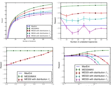
of gradient descent is set to T = 100, one expert trajectory is provided (l = 1), and the number of unsupervised trajectories is set to u = 20 with ν = 0.5. In order to study the impact of different parameters on the algorithms, we first report results where we fix all the above parameters except one and ana-lyze how the performance changes for different values of the selected parameter. In particular, in Fig. 1, while keeping all the other parameters constant, we compare the performance of MaxEnt-IRL, different setups of MESSI, and MESSIMAX by varying different dimensions: 1) the number of iterations of the algorithms, 2) the number of unsupervised trajectories,
3)the distribution Pµ1 by varying ν, and 4) the value of
pa-rameter λ. We then report a comparison with the MaxEnt-IRL with all trajectories and EM-MaxEnt algorithm in Fig. 2.
0 20 40 60 80 100 Number of iterations −10 −9 −8 −7 −6 −5 −4 −3 −2 −1 Re wa rd MaxEnt MESSIMAX MESSI with distribution Pµ1
MESSI with distribution Pµ2
MESSI with distribution Pµ3
5 10 15 20 25 30 35 40 45 Number of unlabeled trajectories −4.5 −4.0 −3.5 −3.0 −2.5 −2.0 −1.5 −1.0 R ew ar d 0.0 0.2 0.4 0.6 0.8 1.0 Parameter nu −5.0 −4.5 −4.0 −3.5 −3.0 −2.5 −2.0 −1.5 −1.0 R ew ar d MaxEnt MESSIMAX MESSI with distribution Pµ1
10−3 10−2 10−1 100 parameter lambda −12 −10 −8 −6 −4 −2 0 R ew ar d MaxEnt MESSIMAX MESSI with distribution Pµ1
MESSI with distribution Pµ2
MESSI with distribution Pµ3
Figure 1:Results as a function of (from left to right): number of it-erations of the algorithms, number of unsupervised trajectories, pa-rameter ν, and papa-rameter λ.
0 20 40 60 80 100 Number of iterations −14 −12 −10 −8 −6 −4 −2 R ew ar d MESSIMAX MESSI MaxEnt with all trajectories
0 20 40 60 80 100 Number of iterations −14 −12 −10 −8 −6 −4 −2 R ew ar d MESSIMAX MESSI 1 - EM MaxEnt 5 - EM MaxEnt 10 - EM MaxEnt 20 - EM MaxEnt 50 - EM MaxEnt
Figure 2:Comparison of MESSI with MaxEnt-IRL using all
trajec-tories (left) and η-EM-MaxEnt with η =1, 5, 10, 20, 50 (right).
The highway problem. We study a variation of the car
driving problem in Syed [2008]. The task is to navigate a car in a busy 4-lane highway. The 3 available actions are to move
left, right, and stay on the same lane. We use 4 features:
colli-sion(contact with another car), off-road (being outside of the
4-lane), left (being on the two left-most lanes of the road), and right (being on the two right-most lanes of the road). The expert trajectory avoids any collision or driving off-road
while staying on the left-hand side. The true reward θ∗
heav-ily penalizes any collision or driving off-road but it does not constrain the expert to stay on the left-hand side of the road.
θ1penalizes any collision or driving off-road but with weaker
weight, and finally θ2does not penalize collisions. We use the
RBF kernel with σ = 5 as the similarity function and evaluate the performance of a policy as minus the expected number of collisions and off-roads.
Results.In the following, we analyze the results obtained
by averaging 50 runs along multiple dimensions.
Number of iterations. As described in Sec. 2,
MaxEnt-IRL solves the ambiguity of expected feature count match-ing by encouragmatch-ing reward vectors that strongly discriminate from expert’s behavior and other policies. However, while in MaxEnt-IRL, all trajectories that differ from the expert’s are (somehow) equally penalized, MESSI aims to provide
sim-ilar rewards to the (unsupervised) trajectories that resemble (according to the similarity function) the expert’s. As a re-sult, MESSI is able to find rewards that better encode the known expert’s preferences when provided with relevant un-supervised data. This intuitively explains the improvement of both MESSI and MESSIMAX w.r.t. MaxEnt-IRL. In partic-ular, the benefit of MESSIMAX, which only uses trajectories drawn from a distribution coherent with the expert’s distribu-tion, becomes apparent after just a few dozens of iterations. On the other hand, the version of MESSI using trajectories
drawn from Pµ3, which is very different from Pu∗, performs
worse than MaxEnt-IRL. As discussed in Sec. 3, in this case, the regularizer resulting from the SSL approach is likely to bias the optimization away from the correct reward. Like-wise, the versions of MESSI using trajectories drawn from
Pµ1 and Pµ2 lose part of the benefit of having a bias toward
the correct reward, but still perform better than MaxEnt-IRL. Another interesting element is the fact that for all
MaxEnt-based algorithms the reward θt tends to increase with the
number of iterations (as described in Sec. 3). As a result, after a certain number of iterations, the reward reaches the
constraint kθk∞ = θmax, and when this happens, additional
iterations no longer bring a significant improvement. In the case of MaxEnt-IRL, this may also cause overfitting and de-grading performance.
Number of unsupervised trajectories. The performance
tends to improve with the number of unsupervised trajecto-ries. This is natural as the algorithm obtains more informa-tion about the features traversed by (unsupervised) trajecto-ries that resemble the expert’s. This allows MESSI to better generalize the expert’s behavior over the entire state space. However in some experiments, the improvement saturates af-ter a certain number of unsupervised trajectories are added.
This effect is reversed when Pµ3 is used since unsupervised
trajectories do not provide any information about the expert and the more the trajectories, the worse the performance.
Proportion of good unsupervised trajectories.MESSI may
perform worse than MaxEnt-IRL whenever provided with a
completely non-relevant distribution (e.g., Pµ3). This is
ex-pected since unsupervised trajectories together with the simi-larity function and the pairwise penalty introduce an inductive bias that forces similar trajectories to have similar rewards. However, our results show that this decrease in performance is not dramatic and is indeed often negligible as soon as the distribution of the unsupervised trajectories supports the
ex-pert distribution Pu∗ enough. In fact, MESSI provided with
trajectories from Pµ1 and Pµ2 starts performing better than
MaxEnt-IRL when ν ≥ 0.15. Finally, note that for ν = 1, MESSI and MESSIMAX are the same algorithm.
Regularization λ. The improvement of MESSI over
MaxEnt-IRL depends on a proper choice of λ. This is a well-known trade-off in SSL: If λ is too small, the regularization is negligible and the resulting policies do not perform bet-ter than the policies generated by MaxEnt-IRL. On the con-trary, if λ is too large, the pairwise penalty forces an extreme smoothing of the reward function and the resulting perfor-mance for both MESSI and MESSIMAX may decrease.
Comparison to MaxEnt-IRL with all trajectories.As
ex-pected, when unsupervised trajectoriesΣeare used directly in
MaxEnt-IRL, its performance is negatively affected, even in
the case of Pµ1 and ν = 0.5 as shown in Fig. 2. This shows
how MESSI is actually using the unsupervised trajectories in the proper way by exploiting them only in the regularization term rather than integrating them directly in the likelihood.
Comparison to η-EM-MaxEnt. In our setting,
η-EM-MaxEnt-IRL is worse than MESSI in all but a few iterations, in which it actually achieves a better performance. The de-crease in performance is due to the fact that the unsupervised trajectories are included in the training set even if they are unlikely to be generated by the expert. This is because the
es-timation of θ∗is not accurate enough to compute the actual
probability of the trajectories and the error made in estimat-ing these probabilities is amplified over time, leadestimat-ing to sig-nificantly worse results. Finally, one may wonder why not to interrupt η-EM-MaxEnt when it reaches its best performance. Unfortunately, this is not possible since the quality of the
pol-icy corresponding to θtcannot be directly evaluated, which is
the same issue as in SSIRL. On the contrary, MESSI improves monotonically and we can safely interrupt it at any iteration.
Our experiments verify the SSL hypothesis that when-ever unsupervised trajectories convey some useful informa-tion about the structure of the problem, MESSI performs bet-ter than MaxEnt-IRL: 1) If the expert trajectory is suboptimal and the unsupervised data contain the information leading to a better solution: For example, in the highway experiment, the expert drives only on the left-hand side, while an optimal pol-icy would also use the right-hand side when needed. 2) In the case where the information given by the expert is incomplete and the unsupervised data provide the information about how to act in the rest of the state space: On the other hand, if none of the unsupervised trajectories contains useful information, MESSI performs slightly worse than MaxEnt-IRL. However, our empirical results indicate that the distribution of the
tra-jectories Pu only needs to partially support Pu∗ (ν ≥ 0.15)
for MESSI to perform significantly better than MaxEnt-IRL.
5
Conclusion
We studied apprenticeship learning with access to unsuper-vised trajectories in addition to those generated by an expert. We presented a novel combination of MaxEnt-IRL with SSL by using a pairwise penalty on trajectories. Empirical results showed that MESSI takes advantage of unsupervised trajecto-ries and can perform better and more efficiently than MaxEnt-IRL. This work opens a number of interesting directions for future research. While MaxEnt-IRL is limited to almost de-terministic MDPs, the causal entropy approach [Ziebart et al., 2013] allows to deal with the general case of stochastic MDPs. A natural extension of MESSI is to integrate the pair-wise penalty into causal entropy. Other natural directions of research are experimenting with other similarity measures for trajectories (e.g., the Fisher kernel) and studying the setting in which we have access to more than one expert.
Acknowledgments
This work was supported by the French Ministry of Higher Educa-tion and Research and the French NaEduca-tional Research Agency (ANR) under project ExTra-Learn n.ANR-14-CE24-0010-01.
References
[Abbeel and Ng, 2004] P. Abbeel and A. Ng. Apprentice-ship learning via inverse reinforcement learning. In Pro-ceedings of the 21st International Conference on Machine Learning, 2004.
[Boularias et al., 2011] A. Boularias, J. Kober, and J. Peters. Relative Entropy Inverse Reinforcement Learning. In Pro-ceedings of the 14th International Conference on Artifi-cial Intelligence and Statistics, volume 15, pages 182–189, 2011.
[Chapelle et al., 2006] O. Chapelle, B. Sch¨olkopf, and A. Zien, editors. Semi-Supervised Learning. MIT Press, 2006.
[Erkan and Altun, 2009] A. Erkan and Y. Altun.
Semi-Supervised Learning via Generalized Maximum Entropy. In Proceedings of JMLR Workshop, pages 209–216. New York University, 2009.
[Klein et al., 2012] Edouard Klein, Matthieu Geist, Bilal Piot, and Olivier Pietquin. Inverse Reinforcement Learn-ing through Structured Classification. In Advances in
Neu-ral Information Processing Systems 25, pages 1016–1024.
2012.
[Levine et al., 2011] S. Levine, Z. Popovic, and V. Koltun. Nonlinear Inverse Reinforcement Learning with Gaussian Processes. In Advances in Neural Information Processing Systems 24, pages 1–9, 2011.
[Ng and Russell, 2000] A. Ng and S. Russell. Algorithms for inverse reinforcement learning. In Proceedings of the 17th International Conference on Machine Learning, pages 663–670, 2000.
[Ng et al., 2004] A. Ng, A. Coates, M. Diel, V. Ganapathi, J. Schulte, B. Tse, E. Berger, and E. Liang. Inverted Au-tonomous Helicopter Flight via Reinforcement Learning. In International Symposium on Experimental Robotics, 2004.
[Syed et al., 2008] U. Syed, R. Schapire, and M. Bowling. Apprenticeship Learning Using Linear Programming. In Proceedings of the 25th International Conference on Ma-chine Learning, pages 1032–1039, 2008.
[Valko et al., 2012] M. Valko, M. Ghavamzadeh, and A. Lazaric. Semi-Supervised Apprenticeship Learning. In Proceedings of the 10th European Workshop on Reinforcement Learning, volume 24, pages 131–241, 2012.
[Zhu, 2005] Xiaojin Zhu. Semi-supervised learning litera-ture survey. Technical Report 1530, Computer Sciences, University of Wisconsin-Madison, 2005.
[Ziebart et al., 2008] B. Ziebart, A. Maas, A. Bagnell, and A. Dey. Maximum Entropy Inverse Reinforcement Learn-ing. In Proceedings of the 23rd AAAI Conference on Arti-ficial Intelligence, 2008.
[Ziebart et al., 2013] Brian D. Ziebart, J. Andrew (Drew) Bagnell, and Anind Dey. The principle of maximum causal entropy for estimating interacting processes. IEEE Trans-actions on Information Theory, February 2013.
A
The Grid-world Problem
In this set of experiments, we use a 16 × 16 square grid-world, a variation of the grid-world domain in (Abbeel and Ng, 2004). The agent has 4 possible actions (up, down, left, right) with 70% chance of success and 30% chance of taking a random different action. The grid is divided into 64 macro-states of size 2 × 2 each, which define the feature space f, so that each macro-state has its own characteristic feature that is active when a state within a macro-state is traversed.
A reward vector θ∗ is generated at random and is set as
the true reward of the problem. This reward maps every fea-ture to a strictly negative value, except for 3 randomly chosen
features. θ1and θ2are also generated at random.
In this problem, we use the RBF kernel s(ζi, ζj) =
exp(−kfζi − fζjk/10) to define the similarity between two
trajectories ζi and ζj. This similarity function is completely
general and does not exploit any prior knowledge about the problem. We evaluate the performance of a policy as its ex-pected reward w.r.t. the true reward, i.e., θ>
truefT .
Results are reported in Figs. 3, 4, 5, and 6. The result of the comparison with the η-EM-MaxEnt are reported in Fig. 7.
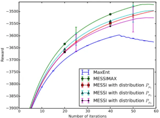
0 10 20 30 40 50 60 Number of iterations −3900 −3850 −3800 −3750 −3700 −3650 −3600 −3550 −3500 Re wa rd MaxEnt MESSIMAX
MESSI with distribution Pµ1
MESSI with distribution Pµ2
MESSI with distribution Pµ3
Figure 3: Results on the grid-world problem as a function of number of iterations of the algorithms.
0 20 40 60 80 100
Number of unlabeled trajectories −1550 −1500 −1450 −1400 −1350 −1300 R ew ar d
Figure 4: Results on the grid-world problem as a function of number of unsupervised trajectories.
0.0 0.2 0.4 0.6 0.8 1.0 Parameter nu −1300 −1290 −1280 −1270 −1260 −1250 R ew ar d MaxEnt MESSIMAX
MESSI with distribution Pµ1
Figure 5: Results on the grid-world problem as a function of parameter ν. 10−3 10−2 10−1 100 parameter lambda −1700 −1680 −1660 −1640 −1620 −1600 −1580 −1560 −1540 R ew ar d MaxEnt MESSIMAX
MESSI with distribution Pµ1
MESSI with distribution Pµ2
MESSI with distribution Pµ3
Figure 6: Results on the grid-world problem as a function of parameter λ. 0 20 40 60 80 100 Number of iterations −1600 −1550 −1500 −1450 −1400 −1350 −1300 −1250 −1200 R ew ar d MESSIMAX MESSI 1 - EM MaxEnt 5 - EM MaxEnt 10 - EM MaxEnt 20 - EM MaxEnt 50 - EM MaxEnt
Figure 7: Comparison between the performance of MESSI and MESSIMAX with the iterative η-EM-MaxEnt with η =
B
The Pit Problem
Initial State
Terminal State Figure 8: The pit domain.
In this set of experiments, we use a 6 × 6 grid world repre-senting an edge surrounding a pit (see Fig. 8). The agent has
4possible actions (up, down, left, right) with 85% chance of
success and 15% chance of taking a random different action. The initial state is the square with coordinate (1, 1) and the terminal state is the square with coordinate (6, 6). The grid is divided in 3 parts that correspond to the 3 different features, the left edge (represented by the white squares in Fig. 8), the right edge (shaded squares), and the pit (the gray squares in the middle).
The objective of the expert is to move from the initial square to the terminal state by avoiding the pit in the mid-dle. The (single) expert trajectory (the black arrow) provided to the learner goes around the pit counter-clockwise. In this case, the unsupervised trajectories are generating as a mixture of trajectories generated from a deterministic policy that goes around the pit either clockwise or counter-clockwise
(basi-cally Pu∗) and trajectories are generated from a policy that
crosses the pit.
The similarity function used in this experiment is
hand-crafted for this domain and is defined as s(ζj, ζk) =
exp(−knj− nkk), where nj denotes the number of change
of direction in the trajectory ζj (for instance going left then
down). This is an example of a hand-crafted similarity func-tion that fits nicely to the problem, since a trajectory is good if and only if it goes around the pit, and thus, turns only once. Since a good trajectory should carefully avoid the pit, for this experiment, we evaluate the performance of a policy by how frequently it crosses the pit, that corresponds to
evaluat-ing the expected feature count fT (obtained after T iterations
of gradient descent) corresponding to the pit. We denote by
fTpitthis value, and report −fTpitas a measure of performance
in the plots of Figs. 9, 10, 11, and 12. The results basically confirm the discussion in other experiments and show an even stronger advantage of MESSI w.r.t. MaxEnt-IRL, i.e., when-ever prior knowledge about the problem is available and a very informative similarity function is chosen, MESSI is very effective in taking advantage of it and significantly outper-forms MaxEnt-IRL. 0 20 40 60 80 100 120 140 160 −5.0 −4.5 −4.0 −3.5 −3.0 −2.5 −2.0 −1.5
Figure 9: Results on the pit problem as a function of number of iterations of the algorithms.
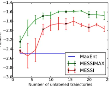
0 5 10 15 20 25
Number of unlabeled trajectories −3.0 −2.8 −2.6 −2.4 −2.2 −2.0 −1.8 −1.6 −1.4 Re wa rd MaxEnt MESSIMAX MESSI
Figure 10: Results on the pit problem as a function of number of unsupervised trajectories.
0 20 40 60 80 100
% of good unlabeled trajectories −3.2 −3.0 −2.8 −2.6 −2.4 −2.2 −2.0 −1.8 −1.6 −1.4 R ew ar d MaxEnt MESSIMAX MESSI
Figure 11: Results on the pit problem as a function of ν.
10-3 10-2 10-1 100 101 102 103 parameter lambda −3.0 −2.8 −2.6 −2.4 −2.2 −2.0 −1.8 −1.6 −1.4 Re wa rd MaxEnt MESSIMAX MESSI