Essays on risk management and financial stability

(1)

HAL Id: tel-01967628

https://tel.archives-ouvertes.fr/tel-01967628

Submitted on 1 Jan 2019

HAL is a multi-disciplinary open access archive for the deposit and dissemination of sci-entific research documents, whether they are pub-lished or not. The documents may come from teaching and research institutions in France or abroad, or from public or private research centers.

L’archive ouverte pluridisciplinaire HAL, est destinée au dépôt et à la diffusion de documents scientifiques de niveau recherche, publiés ou non, émanant des établissements d’enseignement et de recherche français ou étrangers, des laboratoires publics ou privés.

Essays on risk management and financial stability

Saifeddine Ben Hadj

To cite this version:

Saifeddine Ben Hadj. Essays on risk management and financial stability. Business administration. Université Panthéon-Sorbonne - Paris I, 2017. English. �NNT : 2017PA01E003�. �tel-01967628�

(2)

Université catholique de Louvain

Louvain School of Management

Université Paris 1 Panthéon Sorbonne

Ecole de Management de la Sorbonne

PhD dissertation

Essays on Risk Management and Financial

Stability

Saifeddine Ben hadj

President: Pr. Jean-Paul Laurent Université Paris 1 Panthéon Sorbonne

Supervisors: Pr. Isabelle Platten Université catholique de Louvain

Pr. Roland Gillet Université Paris 1 Panthéon Sorbonne

Jury: Pr. Hans Dewachter National Bank of Belgium & KULeuven

Pr. Frédéric Lobez Université de Lille 2

Pr. Mikael Petitjean Université catholique de Louvain et IESEG

(3)

Saifeddine Ben hadj

Essays on Risk Management and Financial Stability PhD dissertation, July 4, 2017

Supervisors: Isabelle Platten and Roland Gillet

Université catholique de Louvain Louvain School of Management Place de l’université

1348 and Louvain-la-Neuve

Université Paris 1 Panthéon Sorbonne Ecole de Management de la Sorbonne Place du Panthéon

(4)

Acknowledgement

Undertaking this PhD has been a truly life-changing experience for me and it would not have been possible to do without the guidance and support that I received from many people.

I would like to first say a very big thank you to my supervisors Prof Isabelle Platten and Prof Roland Gillet for all the support and guidance they provided during the elaboration of this PhD without their constant feedback this PhD would not have been achievable.

Besides my advisor, I would like to thank the rest of my thesis committee: Prof Mikael Petitjean, Prof Jean-Paul Laurent for their insightful comments and encour-agement, but also for the hard questions which incented me to widen my research from various perspectives.

I also thank Prof Hans Dewachte and Prof Frédéric Lobez for carefully reading this thesis and providing valuable feedbacks and comments.

I would like to thank my colleagues in UcL especially in Mons campus for the stimu-lating discussion and all the fun we had. I also address my thanks to my colleagues in the National Bank of Belgium who encouraged me during the last miles of this journey.

Last but not least, I would like to thank my family: my parents and my sisters for supporting me and their prayers throughout writing this thesis and my life in general. My gratitude goes to my wife Mariem the women who made all the differ-ence in my life who supported me, encouraged me and gave me the strength that I needed when I despaired. My thanks go also to little Anass who supported me

(7)

without knowing with his joyful smile and continuously radiating happiness in our home.

(8)

1

Introduction

In the late19thcentury, it was the failure of railroad companies that triggered ma-jor economic crises. Their role as intermediate between miners, producers, and consumers was the cornerstone and booster of economic activity. Nowadays, it is banks and more generally financial institutions that play the leading role in the economy. Some claim that the ability of banks to intermediate between those who are willing to lend and others in need of borrowing is the key determinant of growth and economic welfare. In the absence of this modern system of intermediation, it would be difficult for companies to fulfill their investment needs and for individuals to invest in durable goods and consume non-durable ones. Driven by regulation and the natural survival instinct living in each economic agent seeking profit, banks are investing billions of dollars yearly in their risk management department.

Economic historian reached no consensus about the origin of the concept of risk. However, one story seems to have more proponents than others. It traces back risk to trades between Christian and Arab merchants in the Middle Age and attributes its origins to the middle-eastern language. Italian traders qualify traveling merchan-dise in the middle of the sea as risk having in mind the negative outcome of its loss, while Arabs consider risk in a positive way. In fact, a risk to Arab merchant is the gain that God attributed to them however hard work is still needed to cash it. The missing link in the history of risk is how the positive connotation has transformed into a negative one after crossing the Mediterranean. Despite this little agreement about the origin of the word, it seems that the modern concept of risk in the west-ern civilization emerged with economic development and replaced the notion of dangers and hazards in the circles of businessmen. Later, entrepreneurs stopped considering risk as a fatality and started to develop strategies to mitigate the effect of risk or what we call now risk management.

(9)

Modern risk management in the financial industry started to grow in the second half of the 20thcentury as investment banks ventured into derivatives. Companies saw there a real opportunity to ship uncertainty out of their balance sheet and focus on their core business activities. It is safe to consider investment bankers as profes-sional risk managers. The task turned to be cumbersome for the industry and their supervisors. The latest financial crisis violently demonstrated the impact of incom-plete risk assessment on the viability of the financial system and the continuity of financial intermediation. It also showed how governments efforts to even keel after the storm without proper crisis management plan could lead to a Pyrrhic victory.

Series of financial crises which began from the great depression of the 1930’s to the great recession that peaked in 2008 has given birth to regulation that shaped the modern financial system. The reforms are generally the result of lessons learned by regulators after the storm. From that angle, the latest financial crisis was a great learning experience for economic agents. The first lesson is that the next crisis is unlikely to be the result of over-investment in A-rated Mortgage Bases Securities (MBS). The second and more important lesson is that regulation needs to be re-engineered having in mind the evolutionary characteristic of the financial actors. It is important to marry micro-prudential measures with macro oriented regulations while keeping an eye on international coordination. In fact, the responsibility of financial system stability is a burden that must be shared between individual banks, national governments, and international regulatory organizations.

No later than 1933, the US government established explicit deposit insurance to protect customers’ deposits against future bank runs via the creation of the FDIC. To avoid moral hazard problems, banks agreed to allow regulators monitor their risk-taking behavior. Besides, they were also concerned about the viability of the financial system and the continuity of its services. Despite all the regulatory efforts (or because too much was done according to some) and the evolution of risk man-agement techniques by banks, the 2008 crisis clearly demonstrated that economic agents were unprepared to cushion the negative effects of a full-scale financial cri-sis. More specifically, they acknowledged the existence of imperfections in the risk management techniques and banking regulations.

(10)

At the level of banks, risk managers were unable to estimate correctly the risk that was undertaken by their institutions. Consequently, most of them failed to antici-pate unprecedented market downturns that endangered the viability of their banks. Even the very few which were able to foresee the wave before hitting the shores failed to reckon the scale of the future crisis. This failure is partially due to the oversimplification of risk assessment models that dealt with sizable portfolios of ex-otic derivatives combined with structured products. This complexity led to a lack of understanding of the real level of risk created by those products. In short, financial engineers were highly overrunning risk managers who had trouble keeping up with the increasing complexity of financial instruments.

In the meanwhile, regulators were lacking the tools and technologies to identify the financial institutions which could threaten the stability of the system. In fact, the financial system could be compared to a soccer game played by banks and refereed by regulators. The common features between both games are that players are highly skilled compared to the arbitrator. Nevertheless, a good pair of eyes is enough to detect unfair actions even by the most resourceful players in soccer games. Unfor-tunately, more complex observation tools are required to identify players who are breaking the rules in the financial system. In fact, the main indicator of the impor-tance of a bank to the economy was the size of the institution. National champions were qualified as being too big to fail and benefited from the implicit guarantee that governments will step-in to bail them out in the case of financial distress.

Of course, such superficial analysis of the contribution of banks to a systemic crisis will fail to anticipate critical downturns and could only result in a massive bailout as it was the case in the US and Europe after 2008. In addition, it was also clear to governments that the lack of international coordination of financial regulation was a source of regulatory arbitrage.

In fact, the globalization of the financial markets resulted in the global spread of the financial crisis and when burst it required remedies at the international level. This dissertation is structured into three proposed essays. In each chapter, we choose to tackle the issues related to risk management from a different angle: the point of

(11)

view of individual banks, national regulators and international regulatory institu-tions.

While subjects may seem different, they all try to give answers to the same ques-tion: How should we improve the process of risk management to enhance financial stability at the banks level and more importantly at the national and international level? For instance, at the level of banks, we propose technical solutions to recon-cile the flexibility of risk management assessment models with the feasibility and real-time implementation of those models. In the upper layer of risk management i.e. regulators, we propose to provide them with tools that can detect hazardous innovation in the financial system without the need of the costly thorough analysis of individual bank positions. Finally, given the fragmentation of regulatory bodies at international or even national levels, we propose a model of strategic interac-tion between different regulators. The chapter aims at studying to what extent collaboration between regulators is beneficial. The titles of each chapter are as following:

• Chapter 1: Non-uniform nested simulation algorithms in portfolio risk mea-surement

• Chapter 2: Financial Institutions Externalities and Systemic Risk: a Tale of Tails Symmetry

• Chapter 3: A game theory approach for systemic risk and international regu-latory coordination

In the first chapter of this dissertation, we focus on the question of improving risk assessment within individual banks and more precisely for those holding portfolios of complex derivatives. In fact, the failure of correct risk assessment during the crisis showed how realistic were the standard assumption. The sacrifices that were made to accuracy in order to obtain a solution in the time limits are no longer acceptable today. To add flexibility to those models, financial engineers are bounded to use simulations that call for the use of computationally greedy algorithms. In this chapter, we question whether the pricing complexity leads inevitably to massive computational spendings in risk management applications. The focus of this chapter

(12)

is the widely used risk Value-at-Risk that requires the use of nested simulations or a two-stage simulations: the outer simulation and the inner simulation. The outer simulation is used to sample risk factors over a given time horizon. The inner simulation reprices the portfolio instruments conditional on the drawn risk factors. We focus on Value-at-Risk because it goes beyond risk management. It is also applied as a limit for managing trading desk in big investment banks and can also be used as an asset allocation criterion.

The core of the first chapter is to improve the direct nested simulation technique to allow for the use of more realistic pricing models while remaining within reason-able computational efforts. These ideas are based on the work of Gordy and Juneja (2010) and inspired from the work of Broadie et al. (2011) on evaluating proba-bilities of large losses. The biggest contribution of this chapter to the literature of computational finance is in the applied methodology. In fact, it is the first technique applied to quantile-based risk measures and it has no prerequisite that could pre-vent its implementation in practice. Later, we provide theoretical justification and numerical implementations of the proposed algorithms to shows its efficiency.

The second chapter focus on a broader concept related to the stability of the fi-nancial system. Regulators from the early 2000 knew the importance of marrying macro and micro-prudential regulations. In fact, what can be considered as a ratio-nal and desirable behavior at the individual level can have serious negative effects on the system. The objective of this chapter is to propose a theoretical and practical framework for identifying and measuring the negative externalities, or the social costs generated by the banking activities. The core of this chapter is to suggest a new framework for assessing the negative impact of the internal decision of banks on the financial system.We develop both a theoretical and an empirical framework to measure those externalities. Our biggest contribution with regard to the litera-ture is in the concept of externalities and the way to measure it. In fact, we argue that any financial activity that creates no negative externalities should not affect the symmetry in the tails of the profit and loss distribution of the banks that take part of this transaction. The perfect example of externalities are the too-big-to-fail implicit guarantee that can distort the P &L distribution. Banks will be keeping the gains resulting from excessively risky positions while they expect governments to

(13)

vene when big losses materialize. Several arguments support the concepts that we propose. First, derivatives contracts are zero-sum games which suggest that some risks are visible on the gains part of their counterparts. The second argument is a historical argument. In fact, most of the hazardous financial innovations resulted in important gains in the start and still lead to heavy losses only visible later in the future. Such outcome suggests that some inter-temporal transfer of risk and present gains are the symptoms of risk taken in a future time. To better understand crises, we argue that it is also important to have a closer look at the build-up phase and we that gains are informative as losses in this case. The last argument is related to risk management within the bank. As gains are the results of a favorable exposure to a set of risk factors, a negative outcome of the same factors will result in losses. The concept of tail symmetry that we introduce is only relevant to the tails as we tolerate skewness that results on different market anticipations.

The last chapter takes a general view of financial stability and questions the impor-tance of international collaboration in the presence of coordination costs. We argue that international coordination is not an obvious decision and regulators should bal-ance costs and benefits to engaging in collaborative efforts. The main incentive for international coordination is the contagion of crises that become more important due to the increasing integration of financial systems. Moreover, history showed that negotiation to share the burden of a crisis_{ex − post is inefficient. This research} proposes a strategic theoretical model based on the concept of contagion used in the biological environments to justify collaboration between similar financial actors in the such as regulators.

The main focus of this chapter is to propose a strategic interaction model between regulators to justify collaboration in the presence of costs. Compared to the rele-vant literature, we contribute both in the choice and the design of the model. First, we extend the famous SIR model (Susceptible/Infected/Recovered or Removed) to the economic context. We propose a unique design in the network literature of banking that takes into account the heterogeneity of banks and the effects that reg-ulation could have on moral hazard. Second, by contrast to the previous works in the financial intermediation literature, we do not consider banks as the atomic unit in the network. We model the financial system as a population of unit values that

(14)

are susceptible to failure. This design allows for the possibility to study general protection measures that are not oriented toward a single financial institution. The results should encourage regulators to consider the international dimension in their expenditures related to regulatory efforts . Depending on the level of interconnect-edness, peripheral countries should help the source country in its regulatory effort beyond the optimal level if decided only by the later. In fact, the country where the crisis starts has no incentive to stabilize more its financial system beyond its selfish optimal level despite that the fact that it would have important positive effects on other countries. We show the importance of a central planner in that context.

After almost ten years since the first sign of the global financial crisis, we believe that the tentative answers provided by each chapter in this document are timely for several reasons.

First, in most advanced economies it seems that the deleveraging cycle is coming to an end. The chances are that banks will take more risk to ensure profits to their shareholders driven by an environment of very low revenue on fixed-income as-sets due to falling interest rates. In such an environment accurately measuring risk grows in importance. The first chapter is very handy in this aspect. Quantile-based risk measures are by far the most widespread technique used by the financial indus-try and it is improving the computational algorithms applicable for those measures the biggest contribution of this chapter to the literature. In fact, techniques applica-ble by practitioner to VaR whic aim at improving directly nested-simulations are in rare in the literature. We show that the algorithms that we develop (called sequen-tial and stratified) for computing risk measures such as the VaR yield significant computational savings. In the simulation exercise, we show the non-optimized uni-form algorithm requires at least twice the effort in the case of the Gaussian portfolio to reach the same level of accuracy. The advantage of is even more pronounced for other more complex settings than the naive algorithm. For example, in the case of a portfolio holding a single position of a basket option, the uniform technique needs between 24 and27.5 more effort to match the performance of the sequential algorithm. The test cases are also more comprehensive than in the literature. The challenge is that the theoretical value of each quantile must be available to compute the performance metrics (MSE) In the chapter, we also provide theoretical evidence

(15)

that the sequential algorithm is superior to its uniform equivalent. In particular, the analytical findings shows that the new technique that we introduce focus the com-putational power around the exact value of the risk measure for the corresponding portfolio. The importance of such a gain is that it allows risk managers to stretch their model to cover risk far in the tails and tackle interconnectedness risk of which the crisis of 2008 revealed the crucial aspect. Moreover, this chapter proposes a technique that does not compete with classic variance reduction techniques. In other words, the latter simulation’s optimization methods can be combined with the algorithms in this chapter. One additional advantage of the sequential and strat-ified algorithms is that with a small tweak they can be useful to compute other types of risk measures that also call for the use of two-steps simulations such as the regulatory stress tests.

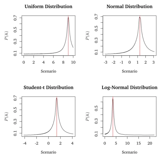
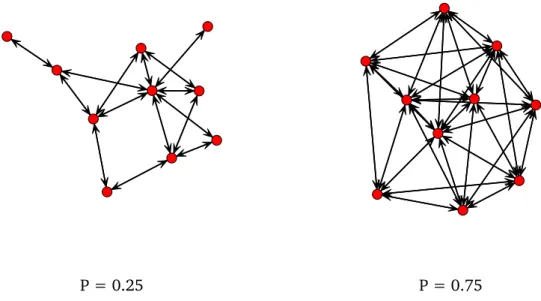
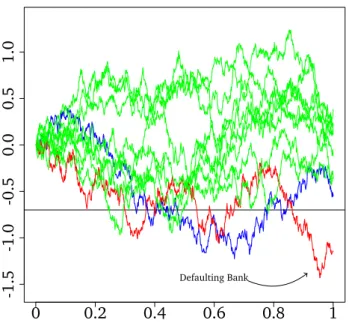
The contribution and lessons drawn from the second chapter are also timely, es-pecially from regulatory aspects. It is indeed critical to build up buffers that can cushion the effect of a financial crisis when the it hits the shores. Moreover, it is important to separate risks that banks can manage via traditional risk management, from those that are due to negative externalities generated by some polluting play-ers in the system. The first type of risk is part of the economic activity of banks and is an engine of economic development. It is the latter that we believe is more dangerous as it is mostly unmonitored and hard to detect. We propose in the third chapter a new framework to detect those invisible risks. The idea is to check the probability of gains to detect the institutions behind such bubble-creating risks. This chapter, shows via three different techniques that extreme gains can be informative about the global health of the financial system. We use a theoretical model in the first part to show that regulators can impose a "fair game" by proposing a weak notion of tail’s symmetry. In that case, systemic crises are limited to unpredictable, out of control events. In addition to this theoretical framework, we also establish via simulations that financial systems are safer when all banks have tail’s symmetry. The model that we use for simulation cover two types of topologies advocated in the literature on banking. The first is a system where the direct connections between banks are the major contagion channel and the second topology is where a common liquidity market centralize transactions between banks. The model that we simulate cannot probably capture all the complexity of a financial system, but the results of

(16)

the simulations are overwhelming and can give hints about the importance of tails symmetry as we advocate it. Finally, we design an empirical measure of externali-ties based on the idea of tail symmetry. We can, via publicly available data, assess the level of externalities that a bank is creating in a period of time. The measure can be computed at the high frequency and can be updated daily. We compare the link between this measure and a proxy for externalities which is the ex-post fines paid by the US banks and show that a measure based on trials symmetry could have higher explanatory power compared to used techniques available in the traditional systemic risk literature.

The third chapter of this thesis deals with the issue of global safety net. In the after-math of the financial crisis, it was argued that collaboration between regulators at the international level was essential to avoid and mitigate, when necessary, financial crises. A question remains unanswerd, what would justify the cost of cooperation especially amid an economic crisis. In the third chapter, we enrich the literature with a special design of the financial system that not only allows answering the pre-vious question but also considers the relationship between regulations and moral hazard. We base the strategic decision of individual regulators on a unique design of the financial system that can cover a multitude of situations where collaboration is possible. The type of situations can range from individual banks pooling up re-sources for times of troubles to cooperation between several regulatory agencies to collaboration between international regulator. In this chapter, we dedicate an important space to the description of the model and the dynamic of the evolution of the crisis inside our model. This is mainly because of the novelty of using this type of model an the economic context. Thanks to this design we show that inter-national coordination is preferable when financial systems are connected enough for contagion to leave sizable effects. We also reveal that it is advisable to subsidize reforms in countries where potentially arise can start and little willingness is shown to engage in stronger regulatory oversight.

Each chapter is structured to be independent of the others. Within each of those chapters, we adopt a classic scheme. We will begin first by a brief motivation. Second, we present an overview of the most relevant literature to the research question. We finally present the methodology and the results.

(17)

(18)

2

A non-uniform nested simulation

algorithms in portfolio risk

measurement

W

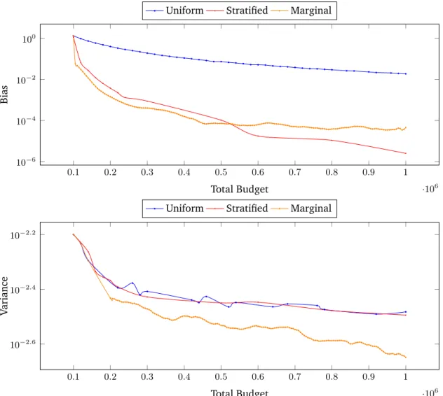
Einvestigate the computational complexity for estimating quantile-based risk measures, such as the widespread Value at Risk for banks and Solvency II capital requirements for insurance companies, via nested Monte Carlo simulations. The estimator is a conditional ex-pectation type estimator where two stage simulations are required to evaluate the risk measure: an outer simulation is used to generate risk-factor scenarios that govern price movements and an inner simulation is used to evaluate the future portfolio value based on each of those scenarios. We propose a new set of non-uniform algorithms to evaluate risk. The algorithms place more importance upon outer scenarios which are more likely to have a direct impact on the estimator and considers the marginal changes in the risk estimator at each additional inner sce-nario. We demonstrate using analytical and experimental settings that our proposed heuristics outperform the uniform algorithm and result in a lower variance and bias with the same initial settings and resources. The results are also robust enough for the multidimensionality of risk factors and the non-linearity of pay-offs.

(19)

Introduction

Despite the theoretical advances made in the field of derivative pricing, a wide range of commonly used derivatives do not fall within range of a pricing formula. Therefore, practitioners have no alternative but to use Monte Carlo simulations and face the constraints of their computational cost. The closer the model is being able to substantially grasp the complexity of the financial system , the more likely is that the time budget needed for an accurate simulation will become excessive. Many simplifications of the models are, therefore, being applied and accuracy is sacrificed to lower the execution time to acceptable limits fixed by the application of the simulation. Consequently, for the purpose of computing large portfolio risk measures, the optimization of simulations is almost inevitable.

The failure of major risk assessment models to protect both big and small investors in the recent years has demonstrated the need for models which are closer to reality. The sacrifices made to accuracy to simplify the models are no longer acceptable. As flexibility should be added to the pricing models, risk practitioners will have their toolbox limited to Monte Carlo simulations for pricing complex products and nested simulations for computing risk measures.

Regardless of the risk measure, the evaluation procedure is usually divided into two stages. Risk scenarios are generated and designed either to reflect normal market conditions and the most probable evolution of the financial market or the contrary the scenarios which are the least likely but bear critical risks for the financial in-stitution. The second stage is to evaluate the portfolio under the condition of the risk scenarios. Because any risk measure is usually to intended account for possi-ble losses within a future time horizon, the two-levels procedure is fated unless a pricing formula exists for each position in the risky portfolio.

In spite of the fact that for risk management application, the time constraint is rather generous the portfolio’s size will affect the task complexity. A second chal-lenge which is overlaid in this particular type of application,it is the use of nested simulation, to evaluate common risk measures such as Value-At-Risk (VaR), Ex-pected Shortfall (ES) or Solvency II capital requirement, on a given horizon. Nested

(20)

simulation calls for the use of two stages of simulations: the outer simulation and the inner simulation. The outer simulation is used to sample risk factors over a given time horizon. The number of required risk factors and the correlation be-tween them justifies the need for Monte Carlo simulations at this level. The in-ner simulation reprices the portfolio instruments conditional on the drawn risk fac-tors.

In this chapter, we question whether the pricing complexities inevitably lead to a large computational burden that may prevent accurate risk assessment in practice. Because some risk scenarios may have no direct impact on the estimator, we show that an ingenious allocation of a relatively small computation budget can yield ac-ceptable levels of variance and bias for portfolio risk measures such as the VaR. We analyze how a fixed computational budget could be allocated across both inner and outer simulations to minimize the Mean Square Error (MSE) of the outcome estimator.

Moreover, the field of application of VaR is not limited to portfolio risk management. Large bank would usually divide its trading activities into trading desks. Manage-ment rules limit the freedom of each desk using quantifiable ceilings. Before the widespread application of VaR, these limits used to be defined in terms of notional limits that were hardly comparable between asset classes. Therefore, the use of a VaR-based trading limit is preferable for managing trading desks. For more details about VaR-based risk limits, refer to Blanco and Blomstrom (1999).

Besides, Cuoco et al. (2008) prove that if VaR is recomputed dynamically using the latest available information, then the risk exposure of trading using VaR is always lower than that computed for the unconstrained traders. Therefore, VaR could also be used as a criterion for asset allocation problems. Again, the dynamic re-evaluation of VaR will require a significant computational budget that could jeopar-dize the application of such a strategy in practice. It is obvious that we are working in relatively small perimeters compared to those of risk management applications, and that means we are no longer limited by the size of the problem. Nevertheless, for trading applications, the time constraint is generally very tight which creates the need for a clever simulation design.

(21)

A second major application of nested simulation in finance is the valuation of Amer-ican options. It is important to remember that AmerAmer-ican options can be exercised at any time until maturity. Hence, the holder of such options is faced with an optimal stopping problem where he must choose the best execution time. The straightfor-ward technique to resolve the issue is by nested simulation. Because a continuous-time stopping problem is burdensome in simulation, most American options are approached as Bermudan options, which have a finite set of execution times. When-ever the set of possible execution times is large enough, the American option could be treated as a Bermudan option. The simulation procedure, which is usually ex-pensive in terms of computational resources, consists in measuring the continuation value at every step on each path via inner simulation to decide whether to exercise the option or continue to hold the option. The outer simulation will be dedicated to sampling different paths. This procedure is not privileged in practice due to its computational cost. However, when dealing with high dimensionalities, such as American style basket options, Monte Carlo repricing seems to be inevitable.

The core of this paper is to present a set of efficient heuristic algorithms to eval-uate quantiles such as VaR. We are focusing our attention on improving the direct nested simulation techniques. Our main purpose is to allow the use of more realistic models in the managing of financial investments.

These ideas are based on the work of Gordy and Juneja (2010) and inspired by the work of Broadie et al. (2011) on evaluating the probabilities of large losses. The main concept behind this paper is that for a two-stage simulation, the additional budget will not have the same marginal improvement from one simulation to an-other. The foremost contributions of this paper to the literature of non-uniform nested estimators are:

1. We will provide a non-uniform nested simulation algorithm for estimating quantile-based risk measures such as VaR and the implementation of the in-ternal model in the Solvency II regulations. The algorithm has no prerequi-site that would prevent practitioners from adopting it. The algorithm will execute the simulation sequentially. The first set of simulations will generate preliminary results. Then extra budget will be allocated, at each step, where

(22)

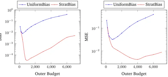
one added inner simulation will have the largest impact on the desired risk measure. The numerical implementation of this estimator demonstrates that bias is reduced dramatically even for relative small additional computational budgets. We also provide a theoretical justification of the efficiency of this technique compared to the standard ones.

2. A second estimator will be proposed. In fact, given that the purpose of the non-uniform estimator is to enhance the uniform algorithm in terms of bias, a budget saving could be generated. However, where the actual level of bias is acceptable, the savings could be considered to generate additional outer scenarios and, consequently, reduce the variance. Therefore, we will present an estimator that will try to balance the bias generated by inner simulations and the variance reducible by increasing the number of outer scenarios.

This chapter will be structured as follows. Section (2.1) will provide a brief liter-ature review. The general simulation framework and notation will be presented in the next section. The third section will be devoted to describing the optimal algorithm proposed for the quantile estimators. Finally, numerical results and con-clusions will be presented in the fourth section.

(23)

2.1 Literature Review

As the measurement is the cornerstone of risk management in a financial institu-tions, it has received the attention of scholars and practitioners for the last few decades. For a general overview of risk measures and risk management in financial markets refer to Crouhy, 2000. Properties and requirements of risk measures were studied in Artzner et al., 1999. They proposed a set of axioms that risk measures are required to satisfy to be deemed a coherent risk measure. It should be noted that, despite the interest given to coherent risk measures in theoretical research, VaR (which is not a coherent risk measure) is, by far, the most widespread risk measure used within the banking industry. However, a number of papers including Cochran et al., 2010 have criticized the axioms of coherence and proposed a dif-ferent classification for risk measures. Their newborn class of risk, called natural risk measures, includes the VaR as defined by the Basel II and Basel III regulations. They also argued that VaR is not contradictory to the principle of diversification as is claimed by Artzner et al., 1999. In fact, according to the VaR criteria, the merger of two portfolios will increase risk only in case of extremely heavy tailed-distribution in which case diversification may not be preferable. Their work seems to provide a theoretical justification for the Basel II and Basel III regulations. The determination of the VaR is also important to compute other risk measures such as the ES defined as the expected loss when the VaR is exceeded. Therefore, even if regulators will shift to the usage of ES for regulatory capitals the determination of the quantiles will remain important and its accuracy will have a direct impact on the precision of the ES. In addition, regulators of financial sectors other than the banking sec-tor, like insurance calls for the use of a quantile-based risk measure. It is the case for example for Solvency II regulation in Europe. For a complete overview on the computational detail of Solvency II capital requirements please refer to Devineau and Loisel (2009) and Bauer et al. (2012). An alternative measure of riskiness has been developed by Bali et al., 2011, who were able to classify portfolios according to their expected return by unit of risk.

The problem of estimating risk measures using nested simulation was first intro-duced by Lee (1998) and Lee and Glynn (2003). Those anthers have began by

(24)

investigating the properties of the uniform nested simulation estimator. Such esti-mators, distribute budget over outer scenarios equally and lead to a constant num-ber of inner simulations. Both authors demonstrated the asymptotic variation of the accuracy of such an estimator where the bias is a function of inner simulation, while the variance of the estimator is inversely proportional to the number of outer scenarios.

The work of Gordy and Juneja (2010) was able to characterize the perfect alloca-tion of budget between inner and outer simulaalloca-tion for uniform nested simulaalloca-tions and has assessed bias for the particular case of the gaussian portfolios. For the continuous case Gordy and Juneja (2010) established that given a total computa-tional budget of Γ the optimal asymptotic mean square error (MSE) is of order Γ−2/3 _{for VaR and expected shortfall. Although, their work is pioneering} concern-ing methodology, it in unclear how to compute the optimal allocation for more complex portfolios where the Profit and Losses’ distribution (P&L) is not theoreti-cally characterized. Guojun Gana (2015) also used similar techniques to value large portfolios of variable annuity (VA) products that provide downside protection from the fluctuation of financial markets in the form of a minimum guarantee.

Authors, such as Longstaff and Schwartz (2001) addressed the problem of nested simulations for pricing American options. They proposed to reduce the computa-tional burden by using a meta-modeling methodology. More precisely, a limited number of inner simulations is generated to estimate a relationship between the price of the options and the risk factors using the least square modeling approach. For a complete overview of the latest techniques of Monte Carlo methods for valu-ing American options and the possible improvement, refer to Bouchard and Warin (2012).

A similar approach is that of Liu and Staum (2010) who proposed the use of stochas-tic kriging for estimating risk measures. Their approach is also a meta-modeling ap-proach that takes into consideration the bias in the estimated values. Kernel-based estimators were studied in the particular case of estimation conditional expecta-tions by Hong, 2009. They demonstrated that the estimator converges at the rate k−min(1,d+24 )whered is the dimension of the risk factor’s vector. This method beats

(25)

the nested simulation only in the case where_{d ≤ 3. However, this technique will} lose its competitiveness in high dimensional simulations.

The work of Broadie et al. (2011) is the closest work to our study. They established an efficient algorithm to allocate budget to inner simulation to compute the prob-ability of large losses. Their development is based on the idea that the marginal change in the risk estimator is not uniform across scenarios when the additional budget for inner simulations is allocated. For risk measures that focus on the tail of the distribution, such us VaR and the probability of large losses, the extreme scenarios are the ones that matter the most.

In our study, we will try to make a similar extension as Broadie et al. (2011) to the work of Gordy and Juneja (2010) but to a more conventional risk measure i.e. the VaR. The main difficulty of our circumstances compared to those of Broadie et al., 2011 is that for evaluation of the probability of large losses the threshold defining extreme losses is known and is expressed in nominal terms. In other words, both the input and the output from the algorithm have the same dimension. In our work, the threshold defining the extreme losses needs to be estimated then updated after each step of the sequential simulation. Our work is also of interest to other applications that need the a conditional expectation of a quantile close to the tail such as the Solvency II capital requirements.

2.2 General Framework

In this section we will present the model framework for the two main application of nested simulation in the financial industry: Value-at-Risk and Solvency II capital requirements. It is also possible to call for the use of nested simulation for other financial application like the valuation of exposures in credit risk measurement. In this paper, we will only focus on regulatory measures. Nevertheless, only a small tweak is needed to be made to the proposed algorithm to be useful for the mentioned application.

(26)

2.2.1 Model Framework for VaR

For consistency purposes, we will follow the model and the notations proposed by Gordy and Juneja (2010).

Let Xt be the vector of v state variables that will determine the asset prices. The

vector should include all the information needed for the pricing operation at time t. In the following, Ftis the filtration generated by Xt. In order to discount future

cash flows, we denote by Bt(s) the value of a unit of currency invested at time t ≤ s

in a risk free money-market account. Given the interest rater then:

Bt(s) = exp

�� s

t r(u)du

�

,

The portfolio that we study is composed of K + 1 positions. The price of each position k will depend on the t, Ftand the legal characteristics of the instrument

priced. Position p0, regroups the set of instruments for which an analytical pricing

function is available. The portfolio is assumed to be held static over the model horizon and maturities Tk are finite for all positions k = 1, · · · , K. The second

assumption will ensure that Monte Carlo pricing is always possible for the positions with no proposed analytical formula.

LetCk(t) be the cumulative cash flow for the position k over the time horizon (0, t].

Notice that conditional on Ft ,Ck(t) is a deterministic function according to the

instrument contractual terms. According to that, the market value of each position is the present discounted expected value of its cash flows under the risk-neutral measureQ. Vk(t) = EQ � � Tk t dCk(s) Bt(s) � � � � �Ft � (2.1) Whenever_{t ≥ T}k, we setVk(t) = 0 2.2 General Framework 21

(27)

Given all those assumptions the portfolio loss, defined as the difference between the present portfolio value and the discounted future values adjusted to interim cash flows, Y can be written as:

Y (H) = K � k=0 � Vk(0) − 1 B0(H) � Vk(H) + � H 0 Bt(H)dCk(t) �� (2.2)

Here the present time is normalized to 0 and the model horizon is H. An implicit assumption is that the interim cash flows received at time t, t < H are reinvested in the money market until time H. However, other conventions could be easily adopted. Moreover, no portfolio weights are used in this model as positions are expressed in currency units.

The combination of equations (2.1) and (2.2) illustrates the necessity of nested simulations. Observe that by construction, Monte Carlo simulation is inescapable for pricing position_{k where k �= p}0. Therefore, repricing via equation (2.2) is only

possible via simulation. Moreover, instruments value at time H and interim cash flows up to the horizon H are conditioned to the choice of the filtration Ft. Once

again, simulation is the only way through this problem, where different filtrations will be generated in order to obtain a vision of the loss distribution function.

Because the value of a position k at time H is simply a conditional expectation that does not depend on future cash flows of other positions (see equation(2.1)), it should be noted that inner simulations can be run independently across position. This could have two benefits in practice. First, it will be possible to run parallel repricing for the distinct positions in the portfolio and take advantage of the ad-vancing parallel computing hardware. Second, this will ensure the diversification of pricing error among different positions and lead to less biased portfolio measures. We will also assume that the initial pricesVk(0) are already known and can be taken

as constant in our problem.

2.2.2 Simulation Framework for VaR

In this section, we will develop the notations needed to illustrate the simulation process. The simulation is nested. More precisely there is an outer step in which

(28)

we simulate scenarios up to the time horizon H. In each trial in the outer step, a second simulation called the inner simulation is needed to reprice each position (except the positionp0by construction).

In what will follow,L will represent the number of trials in the outer simulation. In each of these trails we will execute the following steps:

1. Simulate a pathXt for t ∈ (0, H] under the physical measure. Let ξ be the

realisation of random variables (Xt : 0 < t ≤ H). Hence, ξl represents the

generated information in the outer steps of triall.

2. Evaluate the accrued value atH of the interim cash flows.

3. Evaluate the price of each position at H and this by applying the following rule

a) Closed-form price for positionp0 atH

b) Simulation withNl inner steps trials for time period(H, Tl]. The inner

paths are simulated under the risk neutral measure.

4. Sum both the accrued value of cash flows and the estimated value at time H and discount everything back to time0. The estimate loss is then ˜Y (ξi)

0 H T Time t ξl ξ1 ξL Zi Z1 ZNk

Fig. 2.1.: Illustration of the Nested Simulation sampling

Figure (2.1) illustrates the idea of the simulation and its nested aspect. Step (1) in the previous procedure is shown in the figure in the time horizon [0, H]. Then, starting from a generated scenario ξl, each position is repriced using the second

sim-ulation as specified in the step 3(b) up to the time horizon T . Using this procedure, the value of each position at timeH will be the mean of the position following the generated path in the inner simulation. The inner Monte Carlo estimator is

(29)

ased. However, its inaccuracy will engender bias in the overall estimator of the risk measure.

2.2.3 Estimating Value-at-Risk

We will now go into more details regarding the problem of efficiently estimating the Value-at-Risk for the loss function_{Y . For a target insolvency probability α, α ∈ [0.1]} , VaR is the valueyα given by :

yα= V aRα[Y ] = inf {y : P (Y ≤ y) ≥ 1 − α} (2.3)

As specified before, the nested simulation generates samples ( ˜Y (ξ1), · · · , ˜Y (ξL)).

We sort these draws as ˜Y_[1] _{≥ · · · ≥ ˜}Y_[L]. ˜Y_�αL� provides an estimate of yα �a�

donates the integer ceiling of the real numbera.

The focus of our work is the efficiency of the estimator. Therefore, we will begin by characterizing the mean square error (MSE). MSE is a conventional measure of the performance of the nested simulation estimator. The objective of this paper is to minimize the MSE.

The MSE E[( ˜Y[αL]− yα)2] could be decomposed as the sum of a bias and a variance

: E_{[( ˜}_Y_�αL�_{− y}_α₎2_] � �� M SE = V[ ˜Y_�αL�] � �� V ariance +�E_{[ ˜}_Y_�αL�_{− y}_α_]�2 � �� Bias2 (2.4)

For a given computational budget, the problem of estimating Value-at-Risk, beyond the pricing complexity of derivatives, is the trade-off between bias and variance. To compute the most efficient estimator of the quantile-based risk measure the budget must be allocated wisely between the two levels of simulation.

(30)

2.2.4 Estimating Solvency II capital requirements:

In Europe, Solvency II plays the role of Basel III for the insurance industry. The sets of rules in Solvency II aim at improving the solvency of insurance companies. The key element of the Solvency II approach is that the company should hold enough capital at time zero to overcome difficulties that may arise from an unforeseen event in the following year.

Economic Balance Sheet at timet At Et

Lt

WhereAtis the market value of the asset at time t. Et is the equity value at timet

andLtrepresents the liabilities also at timet. The objective of solvency is to ensure

that insurance companies have enough capital to face a bankruptcy situation i.e Et= At− Lt< 0. To compute the value of the economic balance sheet, we need to

introduce the following notation:

(Ft)t≥0 : is the filtration of the available information at time, all the elements

: of the balance sheet are Ftmeasurable

δ_t the discount factor expressed with the risk free ratert.

δt= e−

�t

0 rhdh

Pt the cash flows of liabilities at period t

Rt the profit of the company at time t

(2.5)

Thus, the value of equity and liabilities at time0 are easily computed as:

L0 = EQ  � u≥1 δuPu|F0   (2.6) E0 = EQ  � u≥1 δuRu|F0   (2.7) 2.2 General Framework 25

(31)

The economic capital is then evaluated using the following formula:

C = E0− P (0, 1)q0.5%(E1) (2.8)

With P (0, 1) is the price of a zero coupon of 1-year maturity. The quantity C is the surplus of capital that need to be added to ensure that the condition that may wipe out the entire equity occurs with a probability equal to 0.5%. We should consider that the evaluation ofC needs the knowledge of the quantile of the equity distribution at a future time1. This is very similar to the computation of V aR. In this context we also have that:

E1 = EQ  � u≥2 δu δ₁Ru|F RW 1 + R1   (2.9)

WhereF₁RW is the real world information of the first year.

For more details about the computation of Solvency II capital requirement please refer to Bauer et al. (2012) and Devineau and Loisel (2009). It is important to have a snapshot of the distribution ofE1 to evaluate the desired quantile. For that

purpose, we need to simulate a different set of information FRW

1 . The valuation

of the future return of the company is usually a simulation exercise. In fact, those revenues depend on several risk factor and a set of financial and non-financial vari-ables with complex emended options in the insurance contracts. Both simulations combined is again a situation of nested simulations.

It is important to note that insurance companies are struggling to implement this technique and are resolved to use a more simplified approach that may miss situa-tions that threaten the viability of the company. It is also worth mentioning that the particular case of Solvency II capital requirements is more complex than Basel III requirements in our opinion. In fact, the long time horizon (1 year ) for Solvency II calls for the use of numerous real world scenario to ensure an acceptable level of accuracy. According to a study by Moody’s (Morrison (2009)) as much as 100 000 real world scenarios are required by insurance companies. This number is almost computationally infeasible for a large portfolio of an insurance contract. Therefore,

(32)

the simulation optimization is inevitable. This paper proposes a feasible solution to this kind of problem.

(33)

2.3 Sampling Algorithms

2.3.1 Uniform Sampling

Uniform sampling is perhaps the most obvious way to proceed to a two level simula-tion. The estimator is a function of two variablesL and N . L is the number of outer simulation and N is the number of inner simulations. The estimator is uniform in the sense that the number of inner stage samples is identical for each outer stage scenario. The algorithm is as follows:

Algorithm 1 VaR uniform estimator sampling 1: procedure UNIFORM(L, N )

2: for_{l ← 1, L do}

3: Generate scenario ξl

4: Evaluate the accrued value atH of the interim cash flows 5: Estimate the closed form price for position0

6: Conditioned on the scenario ξlgeneratei.i.d inner samples ˆZl,1, · · · , ˆZl,N

of portfolio losses

7: Compute an estimate of portfolio loss in scenariol ˜Yl= _N1 �Ni=1Zˆl,i

8: end for

9: Compute an estimate of the VaR,yˆα = ˜Y_�αL�

10: end procedure

An asymptotic characterization of the bias and variance of the uniform estimator is possible throughout a set of technical assumptions that will ensure that the higher order partial derivatives could be eliminated when proceeding with a Taylor series expansion to compute an asymptotic version of the bias1as follows:

Gordy and Juneja (2010) established an asymptotic characterization of the bias based upon known properties of order statistics:

Theorem 1 2:

Bias = E[ ˜Y_�αL�_{] − y}α=

θα

N f (yα)

+ oN(N−1) + OL(L−1) + oN(1)OL(L−1) (2.10)

1_{For more information about these technical assumptions and a discussion about their implications}

please refer to Gordy and Juneja (2010).

2_{We say that a function is O}

m(h(x)), if its absolute value is upper bounded by a constant multiplied

by h(x) starting from a sufficiently large m. In the same way, we say that a function is om(h(x)),

if for all � >0 the absolute value of the function is upper bounded by � multiplied by h(x) starting from a sufficiently large m

(34)

Knowing that :

Θ_{(u) =} 1

2f (u)E[σ

2

ξ | Y (ξ) = u]

Wheref denotes the density distribution function of Y and σ2

ξ is the conditional

variance of the error of the portfolio inner pricing (conditioned on ξ). Finally let θα = −Θ�(yα).

With the aid of Theorem 1, we can visualize3 _{that in the case of Value-at-Risk,}

the bias is introduced by the uncertainty of the inner simulation. Consequently, the number of inner simulations determines of the level of bias. Allocating more budget to the inner simulation will increase the accuracy of the inner simulation and, consequently, reduce the bias. However, an increase of1 in the number of inner scenarios will result in an increase ofL in the total budget for uniform estimators.

The number of outer scenarios will be the key factor in variance reduction as increas-ing the number of outer scenarios sampled will decrease the variance. Theorem 2 is an asymptotic characterization of the level of variance

Theorem 2 V_{[ ˜}_Y �αL�] = α_{(1 − α)} (L + 2)f (yα) + oL(L−2) + oN(1)OL(L−1) (2.11)

Theorems (1) and (2), besides characterizing the origin of bias and variance, also allow the convergence rate of the uniform algorithm to be determined. Depending on the application, the convergence speed of both bias and variance may oblige a practitioner to employ significant numbers of both inner and outer scenarios. Conse-quently, for large portfolios, uncontrollable amounts of memory and computational resources are often required to satisfy the industry standards.

3_{The Bias}2 _{is proportional to} 1

N2, as the two parameters θα and f(yα) are not a function of the

simulation parameters. Hence, as the bias could be eliminated by dramatically increasing the number of inner simulation, the inaccuracy introduced by the inner Monte Carlo simulation is the origin of bias

(35)

2.3.2 Optimal Uniform Sampling

Gordy and Juneja (2010) demonstrated that the optimal choice ofL and N could lead to a better allocation of computational budget. In other words, they established the existence of L∗ _and_N∗ _{that minimize the MSE. This result is conditioned by}

the verification of a set of assumptions. Before illustrating the value of the optimal choices, we will first assume the following notations: γ0is the average effort needed

for generating an outer scenario. γ1 will be the average effort needed in the inner

simulation. Thus, the overall computational effort will be Γ= L(N γ1+ γ0)

Specifically, to find the optimal budget allocation between inner and outer simula-tions, we will use the approximation of MSE. It is important to remember that the MSE is the sum ofBias2 and variance detailed in Theorem 1 and Theorem 2. The solution of the following optimization problem will lead to a perfect asymptotic al-location of budget between the inner and outer scenarios. It will also lead to the best possible performance using the uniform algorithm.

minimize L,N θα N f (yα)+ α(1−α) (L+2)f(_y α) subject to L(N γ1+ γ0) ≤ Γ, L, N ≥ 0.

The solution to the problem is :

N∗ = � 2θ2α α_(1−α)γ1 �1/3 Γ1/3_{+ o}_Γ_(Γ1/3₎ and L∗ ₌ �α_(1−α) 2γ2 1θα2 �1/3 Γ2/3_{+ o}_Γ_(Γ2/3₎ (2.12)

The two parameters are then injected into the uniform algorithm to compute an estimator of the VaR.4.

(36)

Despite the importance of the work of Gordy and Juneja (2010), they do not give a practical approach for implementing the simulation, and the optimal allocation so-lution that they present is quite difficult to use in practice as some of the parameters required are not available and must be the object of a simulation. Therefore, the optimal solution could only be used as a benchmark of other simulations designed to compute risk measures and could not be applied to industry problems.

Lee and Glynn (2003), adopted the strategy of using a two-stage simulation to com-pute the distribution of conditional expectations. The output of the first stage is the number of inner and outer simulations to be perform in order to attain the optimal estimator. The second step will be to perform nested simulations to compute the desired loss probability. Their algorithm delivered a small empirical improvement to the crude uniform estimator.

2.3.3 Sequential Simulation

Here,we will present a second family of algorithms studied by Broadie et al. (2011). Their work is focused on the measure of the probability of large loss. Their work is very similar to that of Lee and Glynn (2003), yet concentrates on probabilities far along the tail of the distribution.

Our development is inspired by their methodology and we tried to use similar think-ing process to develop more efficient algorithms to estimate the VaR.

Because the estimator of the VaR is ˆY_�αL�, we can see that only the order of the estimated values and the quantity of the _�αL�thloss matters for the estimator. The basic idea behind our procedure is that an additional scenario will yield the greatest impact whenever it has a much greater probability of changing the order of the esti-mated losses and by consequence a greater probability of affecting the estimator. To explain and illustrate our idea, we will present a simple example. Imagine a setting where a certain number of inner and outer simulations has been performed. The quantile that we seek to estimate, is on the right tail of the distribution. Therefore, obvious allocating additional budget to the outer scenarios where losses are closer to the right tail will have a greater impact to allocate . By contrast, the additional

(37)

of an inner scenario to an outer scenario where the associated loss is located in the left tail will not impact upon the VaR estimate greatly. It is very unlikely that the added scenario will make the loss jump to the level that will alter the quantile estimator on the opposite tail of the distribution. This example illustrates both the concept behind the estimator that we are developing and, in the same occasion, demonstrated the inefficiency of the uniform estimator.

To go further into detail, let us suppose that we have already estimated L outer scenarios usingN0 inner steps. The challenge is to find the best allocation for the

remaining budget Γ_{− L}0(N0γ1+ γ0).

Without any loss of generality, let us suppose that the set ˆYB

ξ1(k1), · · · , ˆY

B

ξL(kL) is non

decreasing. Where ˆY_ξB

l(kl) is the loss estimated using klinner steps and conditioned

to scenario ξl. The overall budget consumed for the simulation at this stage is

B = L0(N0γ1+ γ0).

The additional inner scenario will cause a significant if the new loss estimated af-fects the order of the losses around the current estimation using the available simu-lations. To be more specific, let us suppose that for the budget B the scenario ξ� _is

the VaR scenario. In other words,Y(ξ�)B(k�) =V aR(B).ˆ

ˆ

Y_ξB+1_i (ki) will denote the loss estimated for the scenario ξi using a total budget of

B + 1 for the global simulation. The first step is to look for the outer scenario ξk

verifying: � ˆ Y_ξB_k(kk) − ˆV aR(B) � � ˆ Y_ξB+1 k (kk) − ˆV aR(B) � < 0 (2.13)

Equation (2.13) ensures that the loss evaluated conditioned on scenario ξk will

jump from the right side of the estimator when adding a single inner scenario or in-versely depending on the initial order of ˆYB

ξk(ki) and

ˆ

V aR(B). In other words, ˆV aR(B) should be inside the segment bounded by ˆY_ξB_k(ki) and ˆYξB+1k (kk) to satisfy condition

(38)

Regardless of the initial and final configuration, we are confident that a scenario satisfying equation (2.13) will have a direct impact on the estimator and therefore, will be more efficiently allocated. In fact, whenever a new inner simulation added to one of the outer-scenarios simulations satisfies condition (2.13), the estimator will see its value changed simply because the outer scenario that generated the VaR loss will be changed. By contrast, not every inner-scenario added can leave its footprint on the value of the estimator. In such a situation, we can say that the additional budget spent to add the corresponding inner scenario was wasted. This is often the case when allocating budget to the outer-scenarios that will result in losses in the left tail of the loss distribution.

However, the main difficulty of this setting compared to the framework of Broadie et al. (2011) and Lee and Glynn (2003), is that for measuring quantile, loss thresholds must be estimated.

It is useful to remember that, in the setting of estimating the probability of large loss, the estimator is:

ˆ α= 1 L L � i=1 1_{{ ˆ}_{Y (ξ}_i_)>c} (2.14) where c is the extreme loss threshold. Both authors evaluated the probability of making an impact on the estimator according to the loss benchmark c which is an input of the estimator and is expressed in currency units. On the other hand, the input for quantile estimation, is a loss probability. Then, as specified in equation (2.13), the benchmark V aR(B) is an estimated value and can bear some inaccu-ˆ racy. Consequently, we should take the uncertainty of the loss estimated in the development into consideration in the sequential simulation.

The uncertainty surrounding the parameter V aR(B) is illustrated in the value ofˆ ˆ

σ_i, the estimated standard deviation of loss conditioned on a scenario ξi. σˆi is

considered as a commonly accepted measure of the uncertainty of the conditional expectation. Hence in the algorithm we will seek a scenario that not only change the estimator but also consider the uncertainty errors in the estimator itself. In order to incorporate the estimation error within the first scenario, our evaluation of the probability of having a direct impact upon the estimator by adding a single

(39)

2σ ˜ yα Y˜Bi(ξi) ˜ YBi+1(ξi) Loss P ro ba bi li ty

Fig. 2.2.: Illustration of the Stratified Nested Simulation sampling changing order strategy

without accounting for uncertainty due to the initial configuration of the scenario and the actual loss estimate

2σ ˆ yα YˆBi+1(ξi) ˆ YBi(ξi) Loss P ro ba bi li ty

Fig. 2.3.: Illustration of the Stratified Nested Simulation sampling changing order strategy

while accounting for uncertainty due to the initial configuration of the scenario and the actual loss estimate

inner scenario will depend on the initial settings. In fact, we will distinguish two different configurations:

• | ˆV aR(B) − ˆYB

ξi(ki)| > ˆσiconfiguration illustrated in figure 2.2.

In this case, we can say with an acceptable level of confidence that the loss generated by the outer scenario ξ is greater (or smaller) than the actual value of the quantile we are trying to estimate using the computational budgetB. Our certainty is derived from the fact that the loss ˆY_ξB_i(ki) is outside the

un-certainty region of the estimatorV aR(B). Therefore, in this setting, there isˆ no need for special treatment to deal with the bias in the estimator.

• | ˆV aR(B) − ˆY_ξB_i(ki)| ≤ ˆσiconfiguration illustrated in figure 2.3

In fact, whenever the loss associated with a given outer scenario ξk is within

the domain of uncertainty, the scenario is still a candidate for the _�αL�th scenario and consequently V aR = ˆˆ Y_ξB

(40)

remedy is to account for inner scenarios that will have the maximum amount of changes to the actual loss estimated conditioned to a given outer scenario. In other terms, we will try to maximize the chances to jump over yˆα ± ˆσi

depending on the initial position of the loss-estimate under consideration and the current estimator of the VaR. The previous treatment will maximize the chances that an order change will occur, and this jump is more likely to be considered relative to the real value of the VaR. In other terms, we are hoping to identify an allocation of the additional inner scenario that may clear the fog and position the loss outside the uncertainty domain([ˆyα− ˆσi, ˆyα+ ˆσi]).

If we were to perform the additional sample in a given scenario ξi, this would result

in a new loss estimate given by:

ˆ Yξi(ki+ 1) = 1 ki+ 1 ki+1 � j=1 ˆ Zi,j = 1 ki+ 1 ˆ Zi,k+1+ ki ki+ 1 ˆ Yξi(ki) (2.15) ˆ

Zi,j is the value of the simulated inner scenario j corresponding to the outer

sce-narioi.

This additional sample will have maximum impact if it changes the order of the set of loss estimators. The event of sample order change, according to the previous condition when considering uncertainty, will be called event A. At this level, it is easy to see that a is a union of two disjointed events: A1 and A2. Where A1 is

the settings where the uncertainty domains of the scenario and the VaR estimator determined by the corresponding standard deviation are overlapping. A2 is the

case where both the estimator of the VaR and the loss conditioned of a scenario are different enough to ignore the effect of uncertainty.

Noting thatd = ˆσ_�αL�andm = ˆyαObserve that:

P_(A₁_{) = P}�_{| ˆ}_Y_ξ i(ki+ 1) − m| ≥ d � � �| ˆYξi(ki) − m| ≤ d) � (2.16) P_(A₂_{) = P}��_Yˆ_ξB k(ki) − m � � ˆ Y_ξB+1 k (kk) − m � ≤ 0�� Yˆξi(ki) − m| ≥ d � (2.17) 2.3 Sampling Algorithms 35

(41)

Using the approximationki(m+d− ˆYξi(ki))+(m+d−µ) ≈ ki(m+d− ˆYξi(ki)) where

E_{[ ˆ}_Z_i,k_{] = µ, the one side Chebyshev inequality, and by denoting σ}_i _{= Var[ ˆ}_Z_i,k_{] we} can establish that:

P_(A₁�� Yˆξi(ki) ≤ m) ≤ � 1 +k2i σ2 i � m + d − ˆYξi(ki) �2�−1 P_(A₁�� Yˆξi(ki) ≥ m) ≤ � 1 +k2i σ2 i � m − d − ˆYξi(ki) �2�−1 (2.18)

And finally, using equivalent development and notation we can establish that:

P_(A₂_{) ≤} � 1 +k 2 i σ_i2 � m − ˆYξi(ki) �2�−1 (2.19)

Before detailing the idea of the optimization algorithm, we will need to divide the set of outer scenarios into three subsetsI1,I2, andI3 where:

I1= � i ∈ 1..L�� m − d ≤ ˆYξi(ki) < m � (2.20) I2= � i ∈ 1..L�� m ≤ ˆYξi(ki) < m + d � (2.21) I3 = � i ∈ 1..L�� | ˆYξi(ki) − m| ≥ d � (2.22)

From this set of equations, we can observe that we have an optimal solution that maximizes the probability of order change (event A). Thus let n∗₁ ,n∗₂ andn3 be a

triplets of integer that satisfies :

n∗₁ = argmin i∈I1 � k2 i σ2 i � m + d − ˆYξi(ki) �2� n∗₂ = argmin i∈I2 � k2 i σ2 i � m − d − ˆYξi(ki) �2� n∗ 3 = argmin i∈I3 � k2 i σ_i2 � m − ˆYξi(ki) �2� (2.23) Recall, that n∗

i ; i = 1..3 is the minimum over 3 disjointed outer scenario spaces

Ii; i = 1..3. Them each minimum is computed over one of the three subspaces.