Publisher’s version / Version de l'éditeur:
Vous avez des questions? Nous pouvons vous aider. Pour communiquer directement avec un auteur, consultez la
première page de la revue dans laquelle son article a été publié afin de trouver ses coordonnées. Si vous n’arrivez
Questions? Contact the NRC Publications Archive team at
PublicationsArchive-ArchivesPublications@nrc-cnrc.gc.ca. If you wish to email the authors directly, please see the first page of the publication for their contact information.
https://publications-cnrc.canada.ca/fra/droits
L’accès à ce site Web et l’utilisation de son contenu sont assujettis aux conditions présentées dans le site LISEZ CES CONDITIONS ATTENTIVEMENT AVANT D’UTILISER CE SITE WEB.
Research Report (National Research Council of Canada. Institute for Research in
Construction), 2003-10-15
READ THESE TERMS AND CONDITIONS CAREFULLY BEFORE USING THIS WEBSITE. https://nrc-publications.canada.ca/eng/copyright
NRC Publications Archive Record / Notice des Archives des publications du CNRC : https://nrc-publications.canada.ca/eng/view/object/?id=53fe3e62-0f2a-421a-8f78-7c726356ccb1 https://publications-cnrc.canada.ca/fra/voir/objet/?id=53fe3e62-0f2a-421a-8f78-7c726356ccb1
Archives des publications du CNRC
For the publisher’s version, please access the DOI link below./ Pour consulter la version de l’éditeur, utilisez le lien DOI ci-dessous.
https://doi.org/10.4224/20378574
Access and use of this website and the material on it are subject to the Terms and Conditions set forth at
Environmental Satisfaction in Open-Plan Environments: 4.
Relationships Between Physical Variables
Newsham, G. R.; Veitch, J. A.; Charles, K. E.; Marquardt, C. J. G.; Geerts,
J.; Bradley, J. S.; Shaw, C. Y.; Reardon, J. T.
Environmental Satisfaction in Open-Plan Environments: 4.
Relationships Between Physical Variables
Newsham, G.R.; Veitch, J.A.; Charles, K.E.;
Marquardt, C.J.G.; Geerts, J.; Bradley, J.S.;
Shaw, C.Y.; Reardon, J.T.
IRC-RR-153
April 2004
Environmental Satisfaction in Open-Plan Environments:
4. Relationships Between Physical Variables
Guy R. Newsham, Jennifer A. Veitch, Kate E. Charles, Clinton J.G. Marquardt, Jan Geerts, John S. Bradley, C.-Y. Shaw, James T. Reardon
Institute for Research in Construction
National Research Council Canada, Ottawa, ONT, K1A 0R6, Canada
IRC Research Report RR-153
Environmental Satisfaction in Open-Plan Environments:
4. Relationships Between Physical Variables
Guy R. Newsham, Jennifer A. Veitch, Kate E. Charles, Clinton J.G. Marquardt, Jan Geerts, John S. Bradley, C.-Y. Shaw, James T. Reardon
Executive Summary
As part of a larger project concerning the design and operation of open plan offices, a field study was conducted to determine the effects of open-plan office design on the indoor environment and on occupant satisfaction with that environment. Measurements were made in nine buildings in six cities; six buildings were in Canada, and three in the US; three were federal buildings, two were provincial buildings, and four were private-sector (high-tech) buildings. A total of 779 employees and their workstations were included in the data set. During a workstation visit, research staff conducted detailed measurements of ventilation, temperature, noise, lighting, and descriptive characteristics of the workstation during a 10-minute period. At the same time, the occupant completed a 27-item questionnaire on a handheld computer concerning their satisfaction with the workplace. The
satisfaction data are analysed in other project reports, this report is concerned only with relationships between the physical variables.
The physical data from the field study were analysed to check that relationships supported those derived from laboratory and simulation (“non-field”) studies in other parts of the project. Where there was a theoretical reason to do so, we also explored the field study data for additional relationships that were not explored in the non-field studies. Overall, the field data showed patterns consistent with the findings of the non-field studies. Therefore, we will continue to use these findings in the development of design software and other guidance for designers. Analyses of acoustics and lighting data supported the relationships and
expectations from other work (e.g., Figure A). In ventilation, the analyses generally showed only small effects, which were sometimes contradictory and not easy to interpret. However, this was also in line with expectations. Other studies have indicated that office design parameters have little effect on ventilation efficiency and thermal comfort when minimal standards for outside air delivery are met. The analyses did reveal some interesting, additional relationships. We found that background noise tended to increase with decreasing workstation size (increasing
occupant density), and decreasing partition height. We also observed that background noise tended to be higher with higher air velocity and lower carbon-dioxide concentrations, perhaps indicating how the operation of the HVAC system might generate noise. Finally, we were able to confirm that temperatures near to windows are generally a little cooler than temperatures in non-windowed workstations, during the winter and spring months.
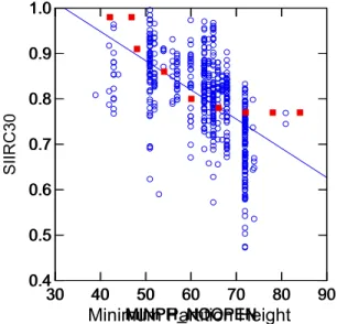
30 40 50 60 70 80 90 0.4 0.5 0.6 0.7 0.8 0.9 1.0 S II R C 3 0 30 40 50 60 70 80 90 0.4 0.5 0.6 0.7 0.8 0.9 1.0 MINPH_NOOPENMINPH_NOOPEN
Minimum Partition Height
Figure A. A comparison between field measured Speech Intelligibility Index, SII (with assumed constant background noise) and results from an analytical model, for variation with partition height. Individual field measurements are blue open circles, and the best linear fit line to these data is also shown.
Table of Contents
1.0 Introduction ... 4 2.0 Method ... 5 2.1 Sites... 5 2.1.1 Building 1 details. ... 6 2.1.2 Building 2 details. ... 7 2.1.3 Building 3 details. ... 7 2.1.4 Building 4 details. ... 7 2.1.5 Building 5 details. ... 8 2.1.6 Building 6 details. ... 8 2.1.7 Building 7 details. ... 8 2.1.8 Building 8 details ... 8 2.1.9 Building 9 details ... 9 2.2 Participants ... 92.2 Physical Dependent Measures ... 9
2.2.1 Cart+chair System... 10
2.2.2. Additional Acoustics Measurements at Night ... 12
2.3 Data Collection Procedure... 13
2.3.1. Measurements at Night ... 15
2.4 Data Analysis Procedure ... 16
3.0 Results ... 18 3.1 Acoustics ... 19 3.2 Lighting ... 25 3.3 Ventilation ... 28 4.0 Discussion... 32 5.0 Conclusions ... 34 6.0 References... 35 Acknowledgements... 36
1.0 Introduction
As part of a larger project (COPE) concerning the design and operation of open plan offices, a field study was conducted to determine the effects of open-plan office design on the indoor environment and on occupant satisfaction with that environment.
Measurements were made in nine buildings in six cities; six buildings were in Canada, and three in the US; three were federal buildings, two were provincial buildings, and four were private-sector (high tech) buildings. A total of 779 employees and their workstations were included in the data set. During a workstation visit, research staff conducted detailed measurements of ventilation, temperature, noise, lighting, and descriptive characteristics of the workstation during a 10-minute period. At the same time, the occupant completed a 27-item questionnaire on a handheld computer concerning their satisfaction with the workplace. The satisfaction data are analysed in other project reports; this report is concerned only with relationships between the physical variables. The methodology of these studies and descriptive data from the various study sites has been detailed elsewhere [Veitch et al, 2002a].
In addition, the COPE project has conducted a number of literature reviews, studies in mock-up office laboratories, and simulation studies (collectively referred to in this report as “non-field” studies) exploring the relationships between office design variables (e.g. workstation size, partition height) and indoor environment conditions (e.g. illuminance, ventilation efficiency, speech intelligibility index). In this report we explore similar relationships in the field study data with two goals:
1. To check the findings against those of the “non-field” studies to ensure there were no important conflicts.
2. To explore relationships that were not, or could not, be addressed in the “non-field” studies.
2.0 Method
The methodology of these field studies and descriptive data from the various study sites has been detailed elsewhere [Veitch et al, 2002a], and only the directly relevant information will be summarized here.
2.1 Sites
Data were collected in nine office buildings, located in large Canadian and American cities. The first three buildings were occupied by government organisations in large Canadian cities, and were visited in 2000. The dataset was expanded in 2002, by including data from four private-sector office buildings (one organisation), and two more government office buildings (one organisation). Three of the buildings were in large Canadian cities, and the remaining buildings were located in two US cities. All buildings, and the specific locations within them, were
selected because they contained open-plan offices occupied by white-collar workers, and because their management was willing to host the visit. During the 2002 data collection, we also intentionally chose buildings that contained smaller workstations and lower partitions, to increase the presence of these workstation characteristics in the overall dataset. A summary of the building characteristics at each site is shown below, in Table 1.
Table 1. Summary of site characteristics.
Bldg. Year
Built City Sector Visited # Floors
Floor plate
(sq.ft.) Lighting HVAC Windows
Sound Masking 1 1977 Ottawa public spring 2000 11 (4 visited) 39,000 (x 2 towers) 4' coffered prismatic fluorescent
ducted air VAV cooling / perimeter hot-water heating non-openable no sound masking 2 1975 Toronto public summer 2000 12 (3 visited) 40,000 4' recessed parabolic cube
ducted air VAV cooling / perimeter convention heating non-openable no sound masking 3 1975 Ottawa public spring 2000 & winter 2000 22 (4 visited) 18,000 4' recessed prismatic (some parabolic)
ducted air VAV cooling / perimeter hot and chilled water heating & cooling non-openable sound masking in use 4 1976 Ottawa private winter 2002 15 (1 visited) 16,000 2’ x 4’ prismatic
ducted air VAV cooling / perimeter hot-water heating
non-operable no sound masking
5 1994 San Rafael private
spring 2002 3 (3 visited) 40,000 2’ x 4’ recessed parabolic
ducted air VAV cooling / hot-water reheat
non-operable sound masking in use 6 1984 San Rafael private
spring 2002 5 (1 visited) 35,000 2’ x 4’ recessed parabolic
ducted air VAV cooling, perimeter hot-water heating non-operable no sound masking 7 1916 (reno-vated 2000) San Francisco private spring 2002 8 (1 visited) 41,000 8’ direct/ indirect
ducted air VAV operable windows sound masking in specific locations 8 1954 Montreal public spring 2002 4 (2 visited) 6,700 50% indirect / 50% 2’x 4’ parabolic
ducted air VAV Perimeter heating
non-operable no sound masking
9 1989/
90 Quebec City public
spring 2002 3 (3 visited) 15,300 1’ x 4’ parabolic fan-coil with occupant-controlled ceiling vents, perimeter electric heating non-operable no sound masking 2.1.1 Building 1 details.
Parts of four floors in the eastern half of this building were visited. Office accommodation at this location was primarily open-plan, with some enclosed offices on the perimeter and at the centre of the floor plan. In the majority of cases, open-plan workstations were formed using free-standing fabric partitions, and free-free-standing furniture elements. Lighting was provided, almost universally, by surface mounted prismatic luminaires housing a single 4ft fluorescent lamp. These luminaires were located at the centre of 5ft x 5ft ceiling coffer elements. Sound masking was not in use at this location. The HVAC system comprised a ducted-air variable air volume (VAV) cooling system, and a perimeter hot-water heating system, both controlled by zone thermostats. Perimeter zones stretched between structural columns along the perimeter (33ft) to a depth of about 10ft; interior zones were up to 30ft x 30ft in size. The building operators controlled zone thermostats. Thermostats were generally fixed at 22oC, although certain thermostats had been adjusted to accommodate local preferences. The VAV system utilised two compartment fans in each tower of each floor. Each fan served approximately half the floor plate, and was capable of supplying up to 25,500 cfm, with the outside air fraction fixed at 10%. Manual controls ensured that the flow rate to the interior zones never fell below 50% of
maximum, and that the flow rate to the perimeter zones never fell below 20% of maximum. These fans were switched off between 6pm – 6am each night; only the fans serving the building lobby and retail floors operated for 24 hours/day.
2.1.2 Building 2 details.
Areas of three floors were visited. Office accommodation at this location was primarily open-plan, with some enclosed offices on the perimeter and at the centre of the floor plan. In the majority of cases, open-plan workstations were formed using systems furniture elements. Lighting was provided, almost universally, by recessed paracube parabolic luminaires housing a single 4ft fluorescent lamp. Orange-painted hollow ceiling beam-like elements formed a 5ft x 5ft ceiling grid, and each of these 5ft x 5ft areas contained one (usually) luminaire at the centre (usually). Sound masking was not in use at this location. The ceiling beams also contained slot air diffusers. The HVAC system comprised a ducted-air VAV cooling system, and a perimeter convection heating system. Zones served by individual VAV boxes were approximately 1500 ft2, though some smaller perimeter zones had been created where solar gain was problematic. The building operators controlled zone thermostats. The target thermostat setting was 22oC, though many thermostats had been adjusted to accommodate local preferences. The building had two main fresh air fans with in-line heating and cooling coils; there was also a cooling coil in the main return air duct. The VAV system utilised two compartment fans on each floor. Each fan served approximately half the floor plate, with the outside air fraction fixed at 15%. Controls ensured that the flow rate to the interior zones never fell below 10% of maximum. These fans were switched off between 6pm – 2am each night.
2.1.3 Building 3 details.
Sections of four floors were visited, two in spring and two in winter. Office accommodation at this location was primarily open-plan, with some enclosed offices at the centre of the floor plan. In the majority of cases, open-plan workstations were formed using systems furniture elements. Lighting was provided, almost universally, by ceiling-recessed prismatic luminaire housing a single 4’ fluorescent lamp, though there were “paracube” parabolic luminaires in a few locations. These luminaires were located in a regular grid on 5ft x 5ft centres. Sound masking was used on all floors at this location. The HVAC system comprised a ducted-air VAV cooling system, and a perimeter hot- and chilled-water system. The perimeter system was locally controlled by occupants. The VAV system was controlled by zone thermostats in the interior; interior zones were up to 15ft x 20ft in size. Zones were originally aligned with office locations, but
rearrangement of office furniture over the years means that this is no longer the case. The building operators controlled interior zone thermostats. Thermostats were initially set at 20-22
oC, although certain thermostats had been adjusted to accommodate local preferences. The
VAV system utilised a total of seven fans, four dedicated to the interior and three to the perimeter. Perimeter fans served South, North-east and North-west zones. The outside air fraction varied with external climate, but never fell below 15 %. These fans were switched off between 6pm – 6am each night.
2.1.4 Building 4 details.
Measurements were taken in various areas of one floor of this building. The office
accommodation was primarily plan, with some enclosed. In the majority of cases, open-plan workstations were formed using systems furniture elements. Lighting was provided, almost universally, by ceiling-recessed 2ft x 4ft, prismatic lens luminaires housing a two 4ft fluorescent lamps, these luminaires were located in a regular grid on 6ft x 10ft centres. There were
supplemental undershelf task lighting in most workstations. The HVAC system comprised a VAV system, with hot water perimeter heating. The VAV system was controlled by pnuematic control thermostats in each zone; the zone sizes are 1200 ft2 on the interior, and every 10 linear ft on the perimeter. Building occupants chose the local thermostat settings. Total air flow to the floor was 40,000 cfm; the outside air fraction varied between 20% and 100%. The system fans were switched off between 9pm – 6 am.
2.1.5 Building 5 details.
Data were collected from all three floors of this building. The office accommodation was primarily open-plan, with some enclosed offices on the 1st floor. In the majority of cases, open-plan workstations were formed using systems furniture elements. Lighting was provided, almost universally, by ceiling-recessed 2ft x 4ft, 18-cell, deep-cell parabolic luminaires housing three 4’ fluorescent lamps, these luminaires were located in a regular grid on 8ft x 12ft centres. There were some supplemental 2ft x 2ft luminaires in some locations, as well as undershelf task lighting. Sound masking was in use in this building. The HVAC system comprised a VAV system, with hot water reheat. The VAV system was controlled by pnuematic control thermostats in each zone; the zone sizes vary based on design, exposure, and usage. The facilities managers set the thermostats at approximately 72 F (22.2 oC). The outside air fraction varied with external climate, but never fell below 20%; free cooling was utilized and outside air fraction could rise to 100% to maximize this. The system fans were switched off between 6pm – 4.30 am each workweek night, and was off all weekend. The organisation we visited at this building had a policy allowing occupants to bring pets, principally dogs, to work. This policy was indicated to be a privilege, and there were requirements for behavioural standards to be met. This organisation also supported work-from-home arrangements.
2.1.6 Building 6 details.
One floor was visited in this building. The office accommodation was a mixture of enclosed offices and open-plan, though measurements were conducted in open-plan offices only. In the majority of cases, open-plan workstations were formed using systems furniture elements. Lighting was provided, almost universally, by ceiling-recessed 2ft x 4ft, 18-cell, deep-cell parabolic luminaires housing three 4ft fluorescent lamps, these luminaires were located in a regular grid on 8ft x 12ft or 8ft x 10ft centres. There was some use of supplemental undershelf task lighting. There was no sound masking system in use in this building. The HVAC system comprised a VAV system, with hot water perimeter coils. The VAV system was controlled by pnuematic control thermostats in each zone; there were typically 3-4 offices per zone. The building managers and tenants interact in setting the thermostats at approximately 70-72 F (21.1-22.2 oC) in summer and 74F (23.3 oC) in winter. Air flow rates were around 1.5-2 cfm/ft2. The outside air fraction was 15-20%. The system fans were switched off between 6pm – 6 am (except Monday when they were started earlier at 4.30 am). The organisation visited at this building also had pets-at-work and work-from-home policies.
2.1.7 Building 7 details.
Measurements were taken on one floor of this building. The office accommodation was entirely open-plan, with a few enclosed conference rooms. Open-plan workstations were formed using systems furniture elements. Lighting was provided, almost universally, by 8ft direct/indirect luminaires housing a single fluorescent lamp, these luminaires were suspended 18 inch. from the ceiling in regular rows. The HVAC system comprised a VAV system only. The VAV system was controlled by zone thermostats in each zone; zones varied in size. The tenants set the thermostats locally at typically 71-73 F (21.7-22.8 oC). Outside air supply was 20 cfm/person, based on 133 ft2/person. The outside air fraction was at least 20% of total air flow. The system fans were switched off between 6pm – 7 am each weekday night. Windows at the building perimeter were openable. The organisation visited at this building also supported work-from-home arrangements.
2.1.8 Building 8 details
Two floors were visited in this building. The office accommodation was mostly open-plan, formed using systems furniture elements. Fifty percent of the lighting in the areas visited was provided by indirect lighting luminaires (2 lamps per 4ft length), suspended 16 inch. From the
ceiling. The remaining lighting was provided by 2ft x 4ft parabolic “paracube” luminaires housing 2 lamps. These luminaires were located in a regular grid on 8ft x 6ft centres.
Workstations also had adjustable “angle-arm” task lights. Sound masking was not in use in this building. The HVAC system comprised a VAV system, capable of supplying 18,265 l/s airflow, and was supplemented with perimeter heating. The VAV system was controlled by direct digital control for each 100 m2 zone. The fraction of outside air varied with external climate, but was never allowed to fall below 17%. Outside airflow was typically around 0.9-1.2 cfm/ft2.
Thermostats were located at the centre of groups of four workstations, and were usually adjusted by occupants. The system was switched off between 6pm and 2.30am each workweek night, and were off all weekend.
2.1.9 Building 9 details
All three floors of this building were visited. The office accommodation was mainly open-plan, formed using systems furniture elements. Lighting was provided by 1ft x 4ft deep-cell parabolic luminaires, housing 2 lamps, with one luminaire assigned for every 50 ft2 of floor area. Sound masking was not in use in this building. The HVAC system used fan coil units to provide local cooling needs. Constant airflow volume was provided meeting a minimum outdoor air supply rate of 10 ls-1/person. Occupants had control of a ceiling diffuser dedicated to their workstation, and could change the direction of airflow, or close the diffuser entirely. Thermostats, to which occupants had access, controlled zones of 400-500 ft2. Perimeter heating was provided by electric baseboard heaters. The HVAC system was turned off at night and on weekends. 2.2 Participants
Participants were the occupants of floors visited by the research team. All occupants present on the visit days were eligible to participate, and approximately 90% of those invited agreed to take part. Table 2 shows the number of occupants who participated at each site.
Table 2. Number of workstations visited at each site.
Site N Full sample 779 Building 1 132 Building 2 160 Building 3 127 Building 4 52 Building 5 85 Building 6 48 Building 7 72 Building 8 47 Building 9 56 2.2 Physical Dependent Measures
Physical measurements were made using two systems. A cart+chair system was used to make measurements of a representative set of variables at each workstation during daytime and at night. Additional equipment was used to make more detailed acoustics measurements at night. These systems are described below.
2.2.1 Cart+chair System
We developed a custom, mobile system to measure the microclimate at the position occupied by an employee in an open-plan office workstation. This system consists of two main
components, the cart and the chair, both wheeled for mobility. The chair served as a platform for the indoor environment sensors. In taking measurements, we temporarily replaced the occupant’s own chair with ours; fabricating our sensor platform in the shape of a chair meant that it had a similar effect on the microclimate as the occupant’s own chair, adding to the validity of the measurements.
Figure 1. The cart and chair used for physical measurements.
Illuminance Sensors (movable) Air velocity Relative humidity Sound Level Temperature probes Radiant temperature Air sample Illuminance cube
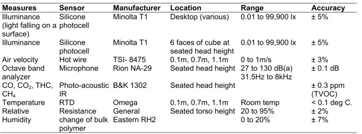
The various sensors mounted on the chair are described in Table 3, and the appearance of the chair is shown in Figure 1. The sensors were chosen to give as broad a characterisation of the indoor environment as possible within a reasonable time (< 15 mins.) and with reasonable mobility (cart+chair system to be moved by two staff through narrow openings typical of open-plan layouts). The selection and location of sensors related to thermal comfort (air temperature, radiant temperature, humidity, and air velocity) were designed to be as similar as possible to those followed in ASHRAE studies [Benton et al., 1990]. Illuminance measurements were taken in defined locations in the workstation (Figure 2), corresponding to locations defined in lighting recommended practice documents (Canada Labour Code, 2002; Illuminating Engineering Society of North America [IESNA], 1993).
The chair was connected to the cart by an “umbilical cord” of sensor lines, power cords, and communications cables. The cart (Figure 1) held a laptop computer, battery and power supply, data acquisitions equipment, and instrumentation for the air quality analysis. A custom data acquisition program on the laptop communicated with all instrumentation on the chair and cart, co-ordinated measurement cycles, and stored the resulting data. The cart also housed a camera, tape measures, open-ended questionnaire envelopes, and other miscellaneous
equipment. The cart was plugged in a wall socket (building’s regular 120V-AC power) overnight to charge the batteries. On a full charge it could operate independently for a full day of
measurements.
Table 3. Description of the various sensors used on the chair.
Measures Sensor Manufacturer Location Range Accuracy
Illuminance (light falling on a surface)
Silicone photocell
Minolta T1 Desktop (various) 0.01 to 99,900 lx ± 5%
Illuminance Silicone photocell
Minolta T1 6 faces of cube at seated head height
0.01 to 99,900 lx ± 5% Air velocity Hot wire TSI- 8475 0.1m, 0.7m, 1.1m 0 to 1m/s ± 3% Octave band
analyzer
Microphone Rion NA-29 Seated head height 27 to 130 dB(a) 31.5Hz to 8kHz ± 0.1 dB CO, CO2, THC, CH4 Photo-acoustic IR
B&K 1302 Seated head height ± 0.3 ppm (TVOC) Temperature RTD Omega 0.1m, 0.7m, 1.1m Room temp < 0.1 deg C. Relative Humidity Resistance change of bulk polymer General Eastern RH2
Seated torso height 20 to 95% 0 to 20%
± 2% ± 7%
Figure 2. Placement of sensor chair and desktop illuminance sensors for daytime measurements.
Chair-based octave band noise level measurements were supplemented by 1/3 octave band
measurements at a sample of locations.
2.2.2. Additional Acoustics Measurements at Night
Measurements of sound propagation between adjacent workstations were performed at night. The source was a small Alpha Mite PSB loudspeaker with directionality similar to that of a human. The receivers consisted of an array of four microphones located at the corners of a square, 46cm on each side.
Measurements were made by radiating a known level of pink noise (equal sound energy in each octave) from the source and measuring the levels at the four microphones in the adjacent workstation. The sound power output of the source was separately measured in a laboratory sound power measurement. This measured sound power output was then used to calculate a reference output level of the source for a distance of 0.9m in a free field (a location with no reflected sound). The microphone signals were transmitted to receivers connected to 4
channels of an 8-channel digital tape recorder, as illustrated in the block diagram of Figure 3(a), and the photo in Figure 3(b). Calibration signals were also recorded on each channel at the beginning and end of each measurement session. The tape recordings were played back under computer control into a B&K 2144 real-time analyzer. The reduction of intruding speech sounds was estimated by subtracting these recorded levels from the known level of the source.
Pink
noise -22 dB
Crown power amplifier PSB
DA38
Nexus
X1 X2 X3 X4
X-wire 1 X-wire 2 X-wire 3
2 3 4
X-wire 4
1
Figure 3. Schematic diagram and photo of equipment for night-time acoustic measurements. (a) Block diagram of equipment used for the night-time sound propagation measurements. The upper half of the figure shows the PSB loudspeaker powered by a Crown power amplifier and the pink noise source. The lower half of the figure shows the 4-microphone array, the Nexus microphone power supply, the X-wire transmitters and receivers and the DA38 digital tape recorder. (b) Photo of equipment.
2.3 Data Collection Procedure
Announcements about the study were sent in advance of the NRC team’s visit, and where possible were coordinated with representatives of both management and employees (e.g., through safety and health committees). During the measurement visits, NRC staff spent full days making individual visits to workstations in the selected areas of the target building. They attempted to visit every occupied workstation in the identified area, returning later if the employee was occupied or momentarily absent.
When the NRC team arrived at an occupied workstation, the members identified themselves and invited the employee to participate. If the employee agreed to participate, he or she was asked to step outside of the workstation in the company of the one of the NRC staff. The NRC staff member took the participant to a nearby location, typically a vacant workstation similar to his or her own, and gave instructions about the questionnaire (because this report is not concerned with questionnaire data, further details on the questionnaire are not provided here). The NRC staff member then left the participant to answer the questionnaire in private, and returned to help the other member of the NRC team with the physical measurements in the workstation. The participant was instructed to return to his or her workstation for assistance from the NRC staff if it were needed.
The measurements in the workstation began with two photographs. The first was a close-up of the computer screen with the screen turned off, principally to identify potential sources of reflected glare. The second photograph was an overall workstation picture, taken from the entrance to the workstation. Both photographs were taken with a Kodak™ DC 260 digital
camera with a wide-angle lens. A small blackboard featuring an ID code for the workstation was included in the photographs, and the same code was recorded on the building plans. In
addition, the photographs were automatically time-stamped, and the time of the visit was recorded on the building plans. These measures helped ensure that all data associated with a particular workstation could be collated later.
Once the instruments were in place, software on the laptop on the cart automatically co-ordinated measurements from the various sensors. Initially, the operator entered the
workstation ID code, and initials identifying him- or herself. The process began with the B&K 1302 taking an air sample for analysis; this process took about 2.5 minutes. While this was happening, NRC staff took measurements of workstation size, partition height and ceiling height, and noted them down for later data entry.
Next the noise level measurements were made; this process took about 1.5 minutes, during this time the NRC team took no actions that might disturb the measurement. The goal was to get a 20-second measurement without intelligible speech sounds (a person talking on the telephone in the next cubicle, for example), as a measure of prevailing background noise. Measurements were repeated 3 times, or until a measurement without speech was captured, whichever
occurred sooner. Other noises occurring during the measurement, such as ventilation noise or noise from outside the building, were noted.
Next, temperature, air speed, humidity and illuminance measurements were taken.
Measurements of all these parameters were taken every 10 seconds, and six measurement cycles were completed in a one-minute period. The last of the six measurements for each variable were shown on the screen, whereas all six measurements, and the mean of all six for each variable, were written to file. On completion, the desktop illuminance sensors were moved to a second location, and the measurements for those sensors were repeated.
Finally, NRC staff entered additional information describing the workstation. These data included relative location of entrance and computer screen, workstation size, partition height and finish, ceiling height, floor finish, lighting type and location, diffuser type and location, whether the VDT had an anti-glare screen, and whether the occupant was wearing headphones when first approached. After completing this screen the operator was prompted to enter any additional comments.
At each stage in this process the operator could visually check the data and redo
measurements if necessary. All data were recorded to a time-stamped text file on the laptop computer. Typically the physical measurements were completed before the questionnaire, in which case NRC staff simply waited for the participant to return to the workstation with the palmtop computer.
Figure 4. Illuminance sensor locations for additional night-time measurements (electric lighting only).
The NRC team then moved on to invite the next available person to participate. There was no set plan as to which employees were approached when, and some work areas were revisited several times to recruit employees who had been unavailable on previous visits to the work area.
2.3.1. Measurements at Night
NRC staff returned after normal working hours (typically 7 – 10 pm) to perform additional measurements with the cart+chair system. These measurements provided baseline data without occupants, and data on the light level provided by the electric lighting system
independent of any daylight contribution. Measurements were made in a subset (around 1/3) of
the workstations that were visited during the day.
Measurements at night with the cart+chair system followed essentially the same protocol as the daytime measurements, with the following exceptions:
• Photographs were not taken, as they would have added little more information to the daytime photographs.
• Additional desktop lighting measurements were made (Figure 4).
• Workstation information was not entered as it would have only duplicated the daytime data. At night we also took the opportunity to take additional photographs not related to a particular workstation (e.g., overall views, luminaires, diffuser types).
At the end of every evening of measurements all data collected with the cart+chair system that day, including questionnaire responses and photographs, were backed up to disk and CD-ROM. Two additional NRC staff conducted the night-time sound propagation measurements. Night-time sound propagation measurements were made in every workstation where dayNight-time measurements had been made (although not necessarily on the same day). The participant’s workstation acted as the receiver workstation, and the source workstation was selected as the adjacent workstation from which speech sounds could most readily propagate.
The sound source was located at the centre of the source workstation and was pointed towards the receiver workstation. The centre of the square receiver array was located at the centre of the receiver workstation. Locating the source and receivers at the centres of each workstation approximated the average of the many possible occupant positions.
These sound propagation measurements were combined with the daytime ambient noise levels measured using the cart+chair system to assess the expected speech privacy between adjacent workstations. A number of other acoustical measures were also derived from these two sets of measurements.
2.4 Data Analysis Procedure
We conducted a series of regressions to test the relationships between important dependent variables and the independent variables expected to predict them. Our primary goal was to test complete models involving multiple predictors, because these account for the interactions of predictor variables. Nevertheless, we did look at single predictor models when comparing to results from the non-field studies, which were able to control conditions such that only a single predictor was varied independently. For example, we predicted the effect of workstation size, partition height and enclosure, and daylight, on illuminance in one 4-predictor model. We also looked at the effect of partition height on illuminance separately to compare the result to simulation studies that had varied only this one independent variable.
Table 4 describes the dependent and independent variables that were addressed in these analyses.
Table 4. Description of the dependent and independent variables addressed in these analyses.
Variable Name Unit (or range)
Description
Dependent Variables
LNOISEA dB(A) A-weighted background noise level at approximately the position of a seated occupant’s head, measured during the day.
SII 0 – 1 Speech Intelligibility Index, calculated from an assumed standard speech level, the sound propagation between workstations measured at night, and LNOISEA
SIIRC30 0 – 1 Speech Intelligibility Index, calculated from an assumed standard speech level, sound propagation between workstations measured at night, and an assumed standard (low level) background noise (RC30) ACO_HI dB(A) A-weighted sound level for 1000-8000 Hz background noise.
ACO_LO dB(A) A-weighted sound level for 16-500 Hz background noise. LOHI_DBA dB(A) ACO_LO – ACO_HI
E_CUBE lux The mean illuminance on the six sides of a cube at approximately the position of a seated occupant’s head, measured during the day. E_DESK lux The mean illuminance on at the four points on the desktop, measured
during the day.
E_DESKUNI 0 – 1 (Maximum of four desktop illuminance points – Minimum of same four points) / Maximum
RTD_H oC Air temperature measured during the day 1.1 m from the ground, at the approximate location of a seated occupant.
AIR_V_H ms-1 Air velocity measured during the day 1.1 m from the ground, at the approximate location of a seated occupant.
REL_HUMID % Relative humidity measured during the day at the approximate location of a seated occupant.
FDCO2 ppm Carbon-dioxide concentration at approximately the position of a seated occupant’s head, measured during the day.
Independent Variables
SQRTAREA ft The square root of the workstation area. The square root is used rather than the area itself because it is better distributed, and better facilitates comparison to non-field studies.
MINPH_NOOPEN inch. The minimum (non-zero) partition height of all partitions making up the cubicle, but excluding any fully open sides.
TIME_CHECK 0 – 1 Fraction of how much of the day had passed when the daytime measurements were made. E.g. 9am = 0.38 (9/24); 4pm = 0.67 (16/24).
PANELS_CAT 0, 1 A measure of enclosure. =1 if the only zero height gap in the partitions was the entrance to the cubicle; =0 if the gap was more extensive.
WINDOW 0, 1 =1 if the cubicle contained an external window; =0 if it did not. DAYLIGHT 0, 1, 2 =2 if the cubicle contained an external window; =1 if it did not have a
window but was within 15ft of a window; =0 if the cubicle was more than 15ft from a window. (treated as a numerical variable in regressions)
DFLOCATE 1, 2 =2 if nearest air diffuser was outside the cubicle; =1 if it was inside the cubicle
MONTH 1, 2, …, 6 Surrogate for external climate =month number for the date on which the daytime measurements were made. Minimum value =1 (January), maximum =6 (June). Note, measurements made in December were given a month value of 1 to preserve the simple ‘higher month, warmer climate’ trend (No measurements were made in July – November.
Univariate outliers for each variable were identified by examining frequency distributions of standardised scores. Scores greater than 3 standard deviations from the mean were excluded from the analysis. Multivariate outliers were detected by examining the values of the
Mahalanobis distance statistic. Cases for which the Mahalanobis distance statistic was greater than the critical value at p<.001 (translated into a critical leverage value, which is the statistic reported by the statistical analysis package used, SYSTAT) were excluded from the analysis. Correlation matrices were examined to check for multicollinearity and singularity.
Circumstances in which items are highly correlated (r>.80) indicate potential multicollinearity problems, because understanding their separate relations to other variables becomes difficult. Items that are only weakly correlated with other variables (r<.30) suggests that the variable is singular, and does not have meaningful relations to other items.
3.0 Results
The results are divided into sections by aspects of the indoor environment: acoustics, followed by lighting, followed by ventilation-related measures. Table 5 shows the descriptive statistics for all of the dependent and independent variables in the analyses.
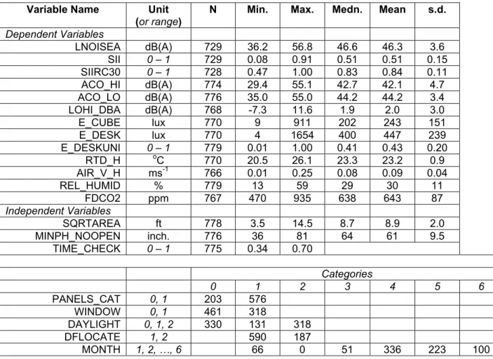
Table 5. Descriptive statistics for variables in these analyses. Values shown for numerical variables are after the univariate outliers have been removed. s.d. = standard deviation.
Variable Name Unit (or range)
N Min. Max. Medn. Mean s.d.
Dependent Variables LNOISEA dB(A) 729 36.2 56.8 46.6 46.3 3.6 SII 0 – 1 729 0.08 0.91 0.51 0.51 0.15 SIIRC30 0 – 1 728 0.47 1.00 0.83 0.84 0.11 ACO_HI dB(A) 774 29.4 55.1 42.7 42.1 4.7 ACO_LO dB(A) 776 35.0 55.0 44.2 44.2 3.4 LOHI_DBA dB(A) 768 -7.3 11.6 1.9 2.0 3.0 E_CUBE lux 770 9 911 202 243 151 E_DESK lux 770 4 1654 400 447 239 E_DESKUNI 0 – 1 779 0.01 1.00 0.41 0.43 0.20 RTD_H oC 770 20.5 26.1 23.3 23.2 0.9 AIR_V_H ms-1 766 0.01 0.25 0.08 0.09 0.04 REL_HUMID % 779 13 59 29 30 11 FDCO2 ppm 767 470 935 638 643 87 Independent Variables SQRTAREA ft 778 3.5 14.5 8.7 8.9 2.0 MINPH_NOOPEN inch. 776 36 81 64 61 9.5 TIME_CHECK 0 – 1 775 0.34 0.70 Categories 0 1 2 3 4 5 6 PANELS_CAT 0, 1 203 576 WINDOW 0, 1 461 318 DAYLIGHT 0, 1, 2 330 131 318 DFLOCATE 1, 2 590 187 MONTH 1, 2, …, 6 66 0 51 336 223 100
3.1 Acoustics
The results of the regressions on Acoustics-related dependent variables (DVs) are summarized in Table 6. For each DV, the initial highlighted section shows the final multiple-predictor model, including the constant, the coefficients (or slopes) associated with predictors (or independent variables, IVs) that are significant in the model, the overall percentage of variance in the DV explained by the model (Radj2), and the F-statistic and degrees-of-freedom for the test (F(df)).
Following that are relevant single-predictor models. Finally, shaded, are models of relationships between acoustic variables and ventilation variables, which we looked at to explore the role of the ventilation system as a substantial source of noise.
Also shown, for each significant IV, is the maximum change in the DV that could be caused by a realistic change in the IV. This is calculated by simply multiplying the coefficient for that IV by the largest realistic change that might be effected in that IV by a designer. We provide this number as a guide to relative magnitude of each effect. The largest changes assumed for this calculation were: SQRTAREA= 5 (equivalent to a change from an 11 ft x 11 ft area cubicle to a 6 ft x 6 ft); MINPH_NOOPEN= 30 (equivalent to a change from a 72 inch high partition to a 42 inch high partition); PANELS_CAT= 1 (equivalent to a change from a cubicle with only one zero-height gap in the partitions, the entrance, to a cubicle with more than one zero-zero-height gap); FDCO2= 400 (equivalent to a change in carbon-dioxide concentration from 900 ppm to 500 ppm); and, AIR_V_H= 0.20 (equivalent to a change in air velocity from 0.05 ms-1 to 0.25 ms-1).
Table 6. Summary of results related to Acoustics dependent variables. “n.s.” indicates the variable was not significant.
DV Const. IV Coeff. R2adj F (df) Mx. Effect.
SIIRC30 1.3169 SQRTAREA n.s. 0.4895 231.5 (3, 718) MINPH_NOOPEN -0.0048 -0.14 PANELS_CAT -0.0955 -0.10 1.0725 SQRTAREA -0.0265 0.2557 250.4 (1, 725) -0.13 1.2059 MINPH_NOOPEN(11) -0.0064 0.3061 239.2 (1, 539) -0.19 FDCO2(sealed) n.s. 0.7912 AIR_V_H 0.3361 0.0165 11.9 (1, 651) 0.07 LNOISEA 55.4325 SQRTAREA -0.3650 0.1577 46.0 (3, 719) -1.8 MINPH_NOOPEN -0.0861 -2.6 PANELS_CAT n.s. 52.1056 SQRTAREA -0.6446 0.1284 108.1 (1, 726) -3.2 53.0600 MINPH_NOOPEN(11) -0.1136 0.0607 36.1 (1, 542) -3.4 51.3401 FDCO2(sealed) -0.0083 0.0397 28.1 (1, 655) -3.3 45.2432 AIR_V_H(sealed) 8.1434 0.0072 5.7 (1, 654) 1.6 SII 0.7083 SQRTAREA 0.0121 0.0936 25.9 (3, 719) 0.06 MINPH_NOOPEN -0.0018 -0.05 PANELS_CAT -0.1126 -0.11 SQRTAREA n.s. MINPH_NOOPEN(11) n.s. 0.2758 FDCO2(sealed) 0.0004 0.0399 28.2 (1, 652) 0.16 AIR_V_H(sealed) n.s. ACO_HI 54.4494 SQRTAREA -0.5566 0.1884 59.6 (3, 755) -2.8 MINPH_NOOPEN -0.0975 -2.9 PANELS_CAT -0.8460 -0.8 50.3649 SQRTAREA -0.9297 0.1605 146.9 (1, 762) -4.6 53.4864 MINPH_NOOPEN(11) -0.1931 0.1026 65.0 (1, 559) -5.8 46.8205 FDCO2(sealed) -0.0080 0.0205 15.2 (1, 680) -3.2 40.5777 AIR_V_H 12.2122 0.0095 7.6 (1, 681) 2.4 ACO_LO 52.3086 SQRTAREA -0.2878 0.1459 44.3 (3, 757) -1.4 MINPH_NOOPEN -0.0914 -2.7 PANELS_CAT n.s. 49.0947 SQRTAREA -0.5575 0.1098 95.3 (1, 764) -2.8 49.2810 MINPH_NOOPEN(11) -0.0874 0.0433 26.4 (1, 560) -2.6 50.0263 FDCO2(sealed) -0.0097 0.0631 46.9 (1, 680) -3.9 AIR_V_H(sealed) n.s. LOHI_DBA -1.8173 SQRTAREA 0.2630 0.0678 19.4 (3, 758) 1.32 MINPH_NOOPEN n.s. PANELS_CAT 0.9076 0.91 -1.1692 SQRTAREA 0.3541 0.0566 47.0 (1, 765) 1.77 -3.1301 MINPH_NOOPEN(11) 0.0877 0.0513 31.3 (1, 560) 2.63 FDCO2(sealed) n.s. AIR_V_H(sealed) n.s.
SIIRC30 is the DV closest to a controlled laboratory measurement; it is derived from a sound propagation measurement made at night, and a standard background noise assumption (rather than that measured during the day). The simple 3-predictor (SQRTAREA, MINPH_NOOPEN, PANELS_CAT) model explains fully 49% of the variance in SIIRC30. The amount of variance explained is not higher because we did not include other predictors in the model that we know to be important but which were not recorded in the field, such as: the sound absorption
properties of the partitions and other cubicle surfaces, the properties of the ceiling, and the location of reflecting surfaces external to the workstation. All of the regressions discussed in this report suffer to an even larger degree from this inevitable lack of inclusion of predictor variables. SQRTAREA is not significant in the overall model, which is surprising given our non-field study results. However, the non-field study regressions are complicated by a high negative correlation between SQRTAREA and MINPH_NOOPEN (r= -0.61) – smaller workstations also tend to have lower partitions, and so associations between a DV and SQRTAREA may be “taken up” by MINPH_NOOPEN, and vice versa. As discussed below, the single-predictor model of SIIRC30 vs. SQRTAREA is significant, and with a relatively large effect.
MINPH_NOOPEN and PANELS_CAT are significant with negative coefficients, this is as expected: taller partitions with more enclosure have lower values of speech intelligibility. The single-predictor model of SIIRC30 vs. SQRTAREA is significant, and the percentage of variance explained is relatively large, at 26%. (Remember, in this single-predictor model, any variance due to differing partition heights at any given workstation size is now ‘unexplained’). The effect of workstation size on sound propagation was measured under controlled conditions in a study in a mock-up office laboratory [Bradley & Wang, 2001]. These data were then used in the development of an analytical model to predict SII in open-plan workstations [Wang &
Bradley, 2001a; Wang & Bradley, 2001b]. We compared the relationship between SIIRC30 and SQRTAREA from the field study with the predictions from the analytical model. For the model we made the following assumptions: cubicles have a square footprint; partition height is equal on all sides at the sample median of 64 inches; the only zero-height opening in the partitions is a single entrance; ceiling height is the sample median of 106 inches; floor type is the sample mode of carpet (SAA= 0.19); ceiling tile is typical of casual field study observations (SAA= 0.55) partitions are typical of casual field observations (SAA= 0.60, STC= 21); and, the background noise level is RC30. The result is shown in Figure 5. The best-fit linear regression line from the field data predicts SIIRC30~ 1 as SQRTAREA tends to 0, which is appropriate. The variation in SIIRC30 with SQRTAREA appears larger (slope steeper) for the field data regression line. However, remember that in the field smaller workstations also tended to have lower partitions. In the output from the analytical model shown in Figure 5 we have assumed the same partition height at all workstation sizes. If we assumed a 54 inch partition at a workstation size of 6 ft x 6 ft, the analytical model predicts SIIRC30= 0.89, much closer to the value predicted by the field data regression line.
For the single-predictor model of SIIRC30 vs. partition height, we chose only those workstations with “full” enclosure (PANELS_CAT= 1); this is indicated by the addition of “(11)” to the
MINPH_NOOPEN variable name. We did this to facilitate comparison to the non-field study results, which modelled a fully enclosed condition. This regression is significant, and the percentage of variance explained is relatively large, at 31%. We compared the relationship between SIIRC30 and MINPH_NOOPEN(11) from the field study with the predictions from the analytical model. The assumption for the model calculations are the same as those above, except that we varied partition height, and fixed workstation size at the sample median of 8.7 ft x 8.7 ft. The result is shown in Figure 6. Note, the analytical model predicts no effect of partition height on SIIRC30 until the partition is at least as high as the speech source, the mouth of a seated occupant, at 48 inches. At this height the field data and analytical output are almost
identical. They continue to be very close over most of the observed range of partition heights, and begin to diverge only at heights exceeding 70 inches, with the trend from the analytical model becoming non-linear. Again, this can be partly explained by the correlation in the field data between workstation size and partition height. If the analytical model is run with larger workstations at higher partitions, the predictions would more closely match the regression line from the field data. For example, for a partition height of 84 inches and a workstation size of 12 ft x 12 ft, the analytical model predicts SIIRC30= 0.72.
SIIRC30 was calculated using a fixed background noise level. However, the field study data suggest that background noise level (LNOISEA) varies with changes in workstation design parameters. The 3-predictor model explains 16% of the variance. Both SQRTAREA and MINPH_NOOPEN are significant with negative coefficients, indicating that background noise tends to increase if workstations are made smaller and partitions are lowered. This is easily explained, given that a substantial fraction of background noise is due to office equipment, non-speech sounds made by occupants, and distant (unintelligible) non-speech. Smaller workstations would increase the density and proximity of such sources, lower partitions would facilitate their propagation. This effect is not currently accounted for in our analytical models, but is worth considering at design time. The single-predictor models add nothing further to the interpretation of effects on LNOISEA. Note that the maximum magnitude of the effects on LNOISEA are in the range of perceivable differences (3dB(A)).
0
5
10
15
SQRTAREA
0.4
0.5
0.6
0.7
0.8
0.9
1.0
S
II
R
C
3
0
0
5
10
15
SQRTAREA
0.4
0.5
0.6
0.7
0.8
0.9
1.0
Figure 5. A comparison between field measured SII (with assumed constant background noise) and results from an analytical model, for variation with workstation size. Individual field measurements are
blue open circles, and the best linear fit line to these data is also shown. Analytical model output is shown by red solid squares.
30
40
50
60
70
80
90
MINPH_NOOPEN
0.4
0.5
0.6
0.7
0.8
0.9
1.0
S
II
R
C
3
0
30
40
50
60
70
80
90
MINPH_NOOPEN
0.4
0.5
0.6
0.7
0.8
0.9
1.0
Figure 6. A comparison between field measured SII (with assumed constant background noise) and results from an analytical model, for variation with partition height. Individual field measurements are blue
open circles, and the best linear fit line to these data is also shown. Analytical model output is shown by red solid squares.
SII is similar to SIIRC30, except that it is calculated using the background noise level measured during the day (LNOISEA). The 3-predictor model explains 9% of the variance.
MINPH_NOOPEN and PANELS_CAT are significant with negative coefficients, this is as expected: taller partitions with more enclosure have lower values of speech intelligibility. However, SQRTAREA has a positive coefficient, though the expectation is that large workstations would have lower speech intelligibility. But remember that SII is a function of sound propagation and the reciprocal of background noise. Larger workstations have lower sound propagation (see SIIRC30 results), but also lower levels of background noise (see LNOISEA results). These two effects will tend to counteract each other, and may explain the unexpected positive coefficient for SQRTAREA. A similar phenomenon will occur for partition height, it may not be enough to reverse the sign of the coefficient, but the magnitude of the effect of MINPH_NOOPEN is clearly smaller than for the SIIRC30 relationship. This probably also explains the lack of the significance in the single-predictor models.
We suggested above that a substantial fraction of background noise was due to office equipment, non-speech sounds made by occupants, and distant (unintelligible) speech. We can partially test this assumption by considering the high and low frequency components of the background noise. The effects of workstation design choices would be expected to be more effective at reducing high frequency sound. This is supported in the regression results. The 3-predictor models for ACO_HI and ACO_LO are both significant, explaining 19% and 15% of the variance respectively. Both SQRTAREA and MINPH_NOOPEN are significant with negative coefficients, indicating that background noise tends to increase if workstations are made smaller and partitions are lowered (as expected). PANELS_CAT is also significant for ACO_HI, and the coefficient for SQRTAREA is approximately twice as large in the ACO_HI model compared to the ACO_LO model. Also, in the single-predictor model with MINPH_NOOPEN, the coefficient is more than twice as large in the ACO_HI model compared to the ACO_LO model.
In a laboratory human factors experiment [Veitch et al, 2002b], we found that the difference between the high and low frequency components of background noise (LOHI_DBA) was predictive of acoustic satisfaction, with higher values of LOHI_DBA tending to yield higher satisfaction. Therefore, we were interested in how it might be affected by office design choices. The 3-predictor model explains 7% of the variance. Both SQRTAREA and PANEL_CAT are significant with positive coefficients, indicating that the low-frequency component tends to increase relative to the high-frequency component if workstations are made larger and more enclosed. This is consistent with the findings above. MINPH_NOOPEN is significant in its single-predictor model, and with a positive coefficient, as expected.
We also explored the possibility of a relationship between ventilation-related and acoustic-related parameters, based on the assumption that the ventilation system is a major contributor to background noise. We also made the reasonable assumption that a “harder working”
ventilation system, in which airflows are higher for longer periods, would make more noise. We did not measure the ventilation system operation directly, so we tried two surrogate measures. These again are based on reasonable assumptions, that higher air flows from the ventilation system will lead to higher air velocities and lower carbon-dioxide concentrations at the locations of measurement. One building in the sample had openable windows that were used during the period of our visit. Open windows would likely increase background noise, and increase air velocity and lower carbon-dioxide concentration, independent of the effect of the mechanical system. Because we were interested in mechanical system noise only, we excluded the data from the building with openable windows from this analysis, this is indicated by the addition of “(sealed)” to the FDCO2 and AIR_V_H variable names. The analyses show that for those DVs directly related to background noise (LNOISEA, ACO_HI, ACO_LO), the single-predictor
regressions are significant, and in the expected direction. The magnitude of the variance explained suggests the FDCO2 is a better single predictor than AIR_V_H.
3.2 Lighting
The results of the regressions on Lighting-related dependent variables (DVs) are summarized in Table 7. Note that when calculating the maximum effect of the IVs there is an additional IV to consider compared to the Acoustics-related results, DAYLIGHT. The maximum change possible in the DAYLIGHT variable is 2 (equivalent to a change from a cubicle having its own window to a cubicle being more than 15 ft from a window).
E_CUBE and E_DESK are both measures of illuminance, and would be expected to behave in a similar way. In some senses, E_CUBE is the more reliable measurement: desktop sensors could be shaded by objects on the desktop, or prevented from being placed in their intended locations; the cube was always placed in the intended, unobstructed, location relative to the occupant’s computer screen. However, E_DESK is very familiar to practitioners, whereas E_CUBE is not, so we performed regressions for both. The overall models contain four predictors, and the result is similar in form for both E_CUBE and E_DESK. In both cases, SQRTAREA, MINPH_NOOPEN and DAYLIGHT are significant predictors, and PANELS_CAT is not. The coefficients are consistent with expectations, and with our non-field studies [Newsham and Sander, 2002; Reinhart, 2002], indicating that illuminance increases with increasing
workstation size, decreasing partition height, and proximity to a window. The 4-predictor model explains a greater percentage of variance in E_CUBE (28%) than in E_DESK (16%), which is perhaps partly explained by the greater reliability in the E_CUBE measure, as described above. The single-predictor models suggest that proximity to a window is the most important predictor of illuminance. The effect of workstation size and partition height was studied using computer simulations [Newsham and Sander, 2002; Reinhart, 2002]. In one set of simulations we
included electric lighting effects only, in another set we looked at daylight penetration explicitly. Therefore to compare the relationships from the field study with the simulation results, we performed separate single-predictor regressions for data from workstations in each of the three DAYLIGHT categories. We also limited the partition height regressions to workstations with “full” enclosure (PANELS_CAT= 1), this is indicated by the addition of “(11)” to the
MINPH_NOOPEN variable name, as this was the design assumption in the simulations. For these single-predictor models there is no significant effect of SQRTAREA on E_DESK. This is surprising, and not consistent with our simulation results. For E_CUBE there is a small effect of SQRTAREA in the non-daylit case (DAYLIGHT=0), the coefficient is positive, consistent with our simulations. There is a larger effect for workstations within 15 ft of a window, but without a window of their own. In this case, the coefficient is negative, this is consistent with our
simulations, because decreasing the size of a cubicle in such circumstances would take it closer to a window.
The single-predictor models related to partition height are generally as expected. The models explain 2-7% of variance, and all have negative coefficients: illuminance increases as partition height decreases. For the E_DESK, DAYLIGHT=0 case we can make a direct comparison to our simulation results. The simulations generated the relative effect of partition height on average desktop illuminance, and indicated that increasing partition height from 30 inch. (no partition above the desktop) to 72 inch would reduce desktop illuminance by ~33%. The regression results indicates a reduction of:
(715 – 5.36•30) – (715 – 5.36•72) x 100% = 41% (715 – 5.36•30)
The comparison is quite good, especially considering all of the unknowns in the field
measurements. Note that the coefficient is substantially larger for the DAYLIGHT=2 case. One likely reason for this is that for a cubicle next to a window, lower partitions would increase the exposure to the windows of neighbours on either side.
The regressions on our measure of illuminance uniformity (E_DESKUNI) were not very successful. The 4-predictor model was not significant, and the single-predictor effects were small and inconsistent. Our simulations indicated that it was difficult to develop general relationships for uniformity, but that illuminance tended to be more uniform for larger
workstations with lower partitions, in a non-daylit scenario. For the DAYLIGHT=0 case, the relationship with SQRTAREA is significant (4% of variance explained), and the coefficient is negative. The definition of E_DESKUNI is such that a lower value indicates greater uniformity, therefore a negative coefficient for SQRTAREA is as expected. For the DAYLIGHT=0 case, the relationship with MINPH_NOOPEN is also significant (5% of variance explained), and the coefficient is negative. This would mean that illuminance becomes more uniform as minimum partition height increases, counter to expectations.
Table 7. Summary of results related to Lighting dependent variables. “n.s.” indicates the variable was not significant.
DV Const. IV Coeff. R2adj F (df) Mx. Effect.
E_CUBE 327.9722 SQRTAREA 14.7876 0.2778 74.5 (4, 760) 74 MINPH_NOOPEN -4.5252 -136 PANELS_CAT n.s. DAYLIGHT 73.4942 147 138.5557 SQRTAREA(day=0) 3.6135 0.0093 4.1 (1, 328) 18 412.5458 SQRTAREA(day=1) -25.0898 0.0839 12.9 (1, 129) -125 SQRTAREA(day=2) n.s. MINPH_NOOPEN(11)(day=0) n.s. 385.9484 MINPH_NOOPEN(11)(day=1) -3.2180 0.0935 9.7 (1, 83) -97 644.5817 MINPH_NOOPEN(11)(day=2) -4.9629 0.0321 9.0 (1, 241) -149 165.2294 DAYLIGHT 80.2873 0.2330 234.6 (1, 768) 161 E_DESK 566.4370 SQRTAREA 16.5366 0.1605 37.5 (4, 760) 83 MINPH_NOOPEN -6.6389 -199 PANELS_CAT n.s. DAYLIGHT 84.2577 169 SQRTAREA(day=0) n.s. SQRTAREA(day=1) n.s. SQRTAREA(day=2) n.s. 710.4607 MINPH_NOOPEN(11)(day=0) -5.2913 0.0676 18.1 (1, 235) -159 764.3216 MINPH_NOOPEN(11)(day=1) -6.1540 0.0905 9.4 (1, 83) -185 1207.9090 MINPH_NOOPEN(11)(day=2) -10.3761 0.0545 15.0 (1, 242) -311 356.9471 DAYLIGHT 92.1285 0.1220 107.8 (1, 768) 184 E_DESKUNI n.s SQRTAREA MINPH_NOOPEN PANELS_CAT DAYLIGHT 0.6050 SQRTAREA(day=0) -0.0206 0.0372 13.7 (1, 328) -0.10 SQRTAREA(day=1) n.s. 0.3361 SQRTAREA(day=2) 0.0129 0.0113 4.6 (1, 315) 0.06 0.7963 MINPH_NOOPEN(11)(day=0) -0.0058 0.0465 12.5 (1, 235) -0.17 MINPH_NOOPEN(11)(day=1) n.s. MINPH_NOOPEN(11)(day=2) n.s. 0.4212 DAYLIGHT 0.0167 0.0045 4.5 (1, 777) 0.03
3.3 Ventilation
The results of the regressions on Ventilation-related dependent variables (DVs) are summarized in Table 8. Note that when calculating the maximum effect of the IVs there are four additional IVs to consider compared to the previous analyses, DFLOCATE, MONTH, TIME_CHECK, and WINDOW. The maximum change possible in DFLOCATE is 1 (equivalent to a change from a cubicle having a diffuser within a cubicle to having a diffuser outside the cubicle); the maximum change possible in MONTH is 5 (equivalent to measurements made in June rather than
January); the maximum change possible in TIME_CHECK is 0.333 (equivalent to
measurements made at 4pm rather than at 8am); the maximum change possible in WINDOW is 1 (equivalent to a change from a cubicle not having a window to a cubicle having a window). In general, the Ventilation-related regressions reveal only small effects related to office design, which are sometimes contradictory and not easy to interpret. However, this is not unexpected. Our non-field studies [Shaw et al., 2003] suggest that office design parameters, in the context of an HVAC system meeting minimal standards for outside air delivery, have little effect on
ventilation efficiency and thermal comfort. [Shaw et al., 1993]
The overall models contain six predictors, with TIME_CHECK and MONTH included to try to account for changes in occupancy and external climate during a day, and changes in external climate during the year, respectively. The six-predictor model for air temperature (RTD_H) explains 15% of the variance, with SQRTAREA, MINPH_NOOPEN, PANELS_CAT,
DFLOCATE, and TIME_CHECK significant, though the maximum magnitude of all effects is no more than 0.5 oC. TIME_CHECK has a positive coefficient, this is expected: occupancy and external temperature tend to increase over the period in which we made our daytime
measurements, both of these effects would tend to increase internal air temperature. DFLOCATE has a positive coefficient, this is expected: the diffuser is generally a source of cooling air, so cubicles with a diffuser above them would tend to be cooler. SQRTAREA has a negative coefficient, this is also expected: larger areas would imply a lower density of heat sources such as occupants and their associated office equipment and desk lamps. Both MINPH_NOOPEN and PANELS_CAT have negative coefficients, suggesting that higher, more enclosing partitions are associated with cooler temperatures. One explanation might be that, for cubicles with a local diffuser, the greater enclosure serves to entrain the cool air within the workstation.
We explored this entrainment hypothesis through single-predictor models. We performed separate single-predictor regressions for data from workstations in each of the DFLOCATE categories (1= diffuser within cubicle; 2= diffuser outside cubicle). We also limited the partition height regressions to workstations with “full” enclosure (PANELS_CAT= 1), this is indicated by the addition of “(11)” to the MINPH_NOOPEN variable name, as this was the design used in our most recent non-field study of ventilation in open-plan office spaces. We see that the effect of workstation size and partition height on temperature is greater (coefficient more negative) for cubicles without their own diffuser, which tends to contradict the entrainment concept. Nevertheless, as seen below, there are other results to support it.
The six-predictor model for air velocity (AIR_V_H) explains only 9% of the variance, with SQRTAREA, MINPH_NOOPEN, DFLOCATE, MONTH, and TIME_CHECK significant, though the maximum magnitude of all effects is no more than 0.03 ms-1. TIME_CHECK has a positive coefficient, this is expected: occupancy and external temperature tend to increase over the period in which we made our daytime measurements, both of these effects would tend to