Building generative models over discrete structures : from graphical models to deep learning

Building Generative Models over Discrete Structures:

From Graphical Models to Deep Learning

by

Georgiana Andreea Gane

Submitted to the Department of Electrical Engineering and Computer

Science

in partial fulfillment of the requirements for the degree of

Doctor of Philosophy in Computer Science and Engineering

at the

MASSACHUSETTS INSTITUTE OF TECHNOLOGY

February 2019

o

Massachusetts Institute of Technology 2019.

Author

...

Signature re

All rights reserved.

clacted

Department of Electrical Engineering and Computer Science

Sppt1

unber 21, 2,018

Signature redacted

C ertified b y ...

... ...

Tommi S. Jaakkola

Thomas Siebel Professor of Electrical Engineering and Computer

Science, and the Institute for Data, Systems, and Society

Thesis Supervisor

Accepted by ...

MASSACH STSNTITUTE OFT ECHNOWOGY

FEB 212019

LIBRARIES

Signature redacted

ILes

&

WI Kolodziej ski

Professor of Electrical Engineering and Computer Science

Chair, Department Committee on Graduate Students

Building Generative Models over Discrete Structures:

From Graphical Models to Deep Learning

by

Georgiana Andreea Gane

Submitted to the Department of Electrical Engineering and Computer Science on September 21, 2018, in partial fulfillment of the

requirements for the degree of

Doctor of Philosophy in Computer Science and Engineering

Abstract

The goal of this thesis is to investigate generative models over discrete structures, such as binary grids, alignments or arbitrary graphs. We focused on developing models easy to sample from, and we approached the task from two broad perspectives: defining models via structured potential functions, and via neural network based decoders.

In the first case, we investigated Perturbation Models, a family of implicit distribu-tions where samples emerge through optimization of randomized potential funcdistribu-tions. Designed explicitly for efficient sampling, Perturbation Models are strong candidates for building generative models over structures, and the leading open questions per-tain to understanding the properties of the induced models and developing practical learning algorithms. In this thesis, we present theoretical results showing that, in contrast to the more established Gibbs models, low-order potential functions, af-ter undergoing randomization and maximization, lead to high-order dependencies in the induced distributions. Furthermore, while conditioning in Gibbs' distributions is straightforward, conditioning in Perturbation Models is typically not, but we theo-retically characterize cases where the straightforward approach produces the correct results. Finally, we introduce a new Perturbation Models learning algorithm based on Inverse Combinatorial Optimization. We illustrate empirically both the induced dependencies and the inverse optimization approach, in learning tasks inspired by computer vision problems.

In the second case, we sequentialize the structures, converting structure generation into a sequence of discrete decisions, to enable the use of sequential models. We explore maximum likelihood training with step-wise supervision and continuous re-laxations of the intermediate decisions. With respect to intermediate discrete repre-sentations, the main directions consist of using gradient estimators or designing con-tinuous relaxations. We discuss these solutions in the context of unsupervised scene understanding with generative models. In particular, we asked whether a

continu-ous relaxation of the counting problem also discovers the objects in an unsupervised fashion (given the increased training stability that continuous relaxations provide) and we proposed an approach based on Adaptive Computation Time (ACT) which achieves the desired result.

Finally, we investigated the task of iterative graph generation. We proposed a vari-ational lower-bound to the maximum likelihood objective, where the approximate posterior distribution renormalizes the prior distribution over local predictions which are plausible for the target graph. For instance, the local predictions may be bi-nary values indicating the presence or absence of an edge indexed by the given time step, for a canonical edge indexing chosen a-priori. The plausibility of each local pre-diction is assessed by solving a combinatorial optimization problem, and we discuss relevant approaches, including an induced sub-graph isomorphism-based algorithm for the generic graph generation case, and a polynomial algorithm for the special case of graph generation resulting from solving graph clustering tasks. In this thesis, we focused on the generic case, and we investigated the approximate posterior's relevance on synthetic graph datasets.

Thesis Supervisor: Tommi S. Jaakkola

Title: Thomas Siebel Professor of Electrical Engineering and Computer Science, and the Institute for Data, Systems, and Society

Acknowledgments

First, and foremost, I thank the Massachusetts Institute of Technology for helping me lay the foundation for my future career by providing the building blocks, through courses, research talks, and research opportunities, and the necessary mentorship, through all the great researchers it has brought in my way.

I thank my advisor, Toinini Jaakkola, for ensuring the quality of the construction at every stage, with enormous patience for good and bad results, for reached and missed deadlines. Through to his unique research insights in a fast-moving field, his hard-working style, his contagious enthusiasm for the unsolved, and, finally, through his sense of humor, Tommi has set himself up to be one of my most influential role models for years to come.

I thank my committee members Leslie Kaelbling, Stephanie Jegelka, and Tamir Hazan for joining me on the construction site, for their insights, their realistic expectations, and their valuable advice on how to shape and prioritize the components of this work. I am particularly grateful to Tamir, a long-term collaborator who morphed into an additional advisor, providing feedback on research, career advice, and hands-on guidance in the completihands-on of this work.

I thank Tommi Jaakkola's lab members Yu Xin, Paresh Malalur, Tatsunori Hashimoto, David Reshef, Jonas Mueller, Vikas Garg, David Alvarez, and Guang-He Lee, whose neighboring constructions motivated and often inspired mine, and the other MIT colleagues, past and present, Yevgeni Berzak, Rahul Gopalkrishnan, Zack Hynes, Karthik Narasimhan, Tahira Naseem, Cristina Sauper, and Adam Yala, for the fun and insightful conversations. I am also grateful to collaborators Jason Weston and Luke Lewitt for the impact they had on my formation as a scientist.

I thank the many friends I made during this process, within and outside the workplace, for being there for me, in spirit, but also in many coffee-shop working sessions, Boston Cream Pie study breaks, or impromptu New York City day-trips. I am grateful to my closest high-school and college friends from Romania, for the emotional support throughout this experience, and for behaving as if we have never been apart while meeting less than once a year.

I thank my family members, whose pride has been unshakeable in front of setbacks, especially my father, who helped me in all things great and small, and my older brother, who has been looking after me in varying ways since I was young, and who has always been an inspiration. Finally, I am grateful to my middle-school teacher Mihaela Rosioru for setting me on this path.

1 Introduction

1.1 M otivation . . . . 1.2 C ontribution. . . . . 2 Generating Discrete Structures via Perturbation Models

2.1 Introduction . . . . 2.2 Related W ork . . . . 2.3 Perturbation Models . . . . 2.4 Implicit Distributions . . . . 2.5 Characterization of Perturbation Models . . . . 2.5.1 Expressive Power of Perturbation Models . . . . 2.5.2 Higher Order Dependencies . . . .

2.5.3 Markov Properties and Perturbation Models . . . .

2.5.3.1 Tree-Structured Perturbation Models . . . 2.5.4 Conditional Distributions . . . . 2.5.4.1 Max-marginals . . . . 2.5.4.2 Conditional Independence . . . . 2.5.5 Perturbation Models and Stability . . . . 2.6 Learning Perturbation Models . . . . 2.6.1 Structured Potential Function Modeling . . . . 2.6.2 Learning Objective . . . . 2.6.2.1 Hard-EM . . . . 2.6.3 Inverse Optimization . . . . 2.6.3.1 Complementary Slackness . . . .

2.6.3.2 Margin-Augmented Inverse Optimization

Contents

21 21 26 29 30 . . . . 33 . . . . 34 . . . . 36 . . . . 38 . . . . 38 . . . . 39 . . . . 41 . . . . 42 . . . . 44 . . . . 46 . . . . 47 . . . . 53 . . . . 56 . . . . 57 . . . . 59 . . . . 60 . . . . 62 . . . . 64 65

2.6.3.3 Examples . . . . 2.6.3.4 Lim itations . . . . 2.7 Empirical Results . . . . 2.7.1 Image Segmentation . . . . 2.7.2 Visual Permutation Learning . . . . 2.7.2.1 Problem Formulation . . . . 2.7.2.2 Model Architecture . . . . 2.7.2.3 Implementation Details for Inverse Optimization 2.7.2.4 Experimental Setup . . . . 2.7.2.5 Understanding Inverse Optimization . . . . 2.7.2.6 Comparison to Previous Work . . . . 2.7.2.7 Potential Extensions . . . . 2.8 D iscussion . . . .

3 Iterative Decoding of Discrete Structures for Scene Understanding 95 3.1 Introduction . . . .

3.2 Scene Understanding with Generative Models . . . . . 3.2.1 Modeling Variable-Length Representations . . . 3.2.2 Scene Understanding Model . . . . 3.3 Continuous Relaxation . . . . 3.3.1 Adaptive Computation Time . . . . 3.3.2 Application to Variable-Length Representations 3.3.3 Lim itations . . . . 3.3.4 Hierarchical Image Generation . . . . 3.3.4.1 Architecture . . . . 3.4 Experimental Evaluation . . . . 3.4.1 Comparison to Attend, Infer, Repeat . . . . 3.4.1.1 Implementation Details . . . . 3.4.1.2 D atasets . . . . 3.4.1.3 Effect of the Topology Loss Scale . . .

68 73 74 75 77 79 80 82 85 88 90 92 93 . . . . 96 . . . . 98 . . . . 99 . . . . 100 . . . . 102 . . . . 102 104 . . . . 106 . . . . 107 . . . . 108 . . . . 110 . . . . 110 110 .... 111 .... 111

3.4.1.4 Comparison to Attend, Infer, Repeat . . . . 3.4.1.5 Hierarchical Approach . . . . 3.5 D iscussion . . . .

4 Iterative Decoding of Discrete Structures for Graph Generation 4.1 Introduction . . . . 4.2 Variational Objective . . . .

4.2.1 Alternative Optimization . . . . 4.2.2 Modeling Power of the Approximate Posterior . . 4.2.3 Connections to Other Graph Modeling Objectives 4.2.3.1 Graph Sequence Modeling . . . . 4.2.3.2 Importance Sampling . . . . 4.2.3.3 Order Matters . . . . 4.3 Graph Sequences . . . . 4.4 Sampling From the Approximate Posterior . . . . 4.4.1 Rejection Sampling . . . . 4.4.2 (Induced) Subgraph Isomorphism . . . . 4.4.3 Feasibility Test . . . . 4.4.4 Polynomially Solvable Special Cases . . . . 4.5 Practical Considerations . . . . 4.5.1 Restricting the Output Size . . . . 4.5.2 Training Efficiency . . . . 4.6 Experimental Evaluation . . . . 4.6.1 D atasets . . . . 4.6.2 Evaluation Metrics . . . . 4.6.2.1 Sequence Modeling Likelihood . . . . 4.6.2.2 _{Graph Modeling (Marginal) Likelihood .} 4.6.2.3 Perplexity Per Edge

4.6.2.4 Evaluation Metrics on Generated Samples 4.6.3 Understanding the GraphRNN Baseline . . . .

. . . . 112 114 115 117 119 123 125 126 128 128 128 129 130 132 133 134 135 137 138 138 139 140 140 141 142 143 144 145 146 .

4.6.4 Implementation Details . . . . 4.6.4.1 Feasibility Test Implementation . . . 4.6.4.2 Eliminating Node Isolation in Partial 4.6.5 R esults . . . .

4.6.5.1 Baseline Results . . . . 4.6.5.2 Visualization . . . . 4.6.5.3 Posterior Sampling . . . . 4.7 D iscussion . . . . A Supplementary Material for Iterative Decoding of

tures for Scene Understanding

A.1 Attend-Infer-Repeat Architecture Details . . . .

Structures. 148 148 149 149 149 152 153 154 Discrete Struc-157 . . . . 157

List of Figures

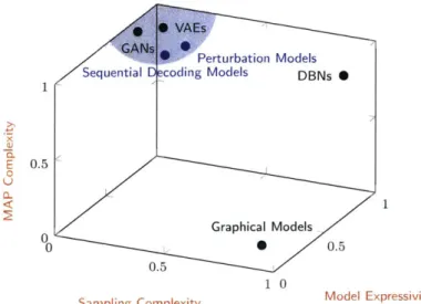
1-1 Illustration of various models along the axes of interest, namely sam-pling complexity, MAP complexity, and model expressivity. In placing the points, we only distinguished between high/low quantities (e.g. whenever sampling is easy, the corresponding point is located close to 0, and whenever sampling is computationally challenging, the corre-sponding point is placed close to 1, with the actual values being selected arbitrarily). The corner highlighted in gray shows the broad focus of the thesis: expressive models that are nevertheless easy sample from. In particular, we explore perturbation models and sequential decoding m odels, shown in blue. . . . . 24

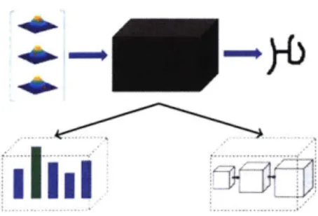
2-1 Broad structure of implicit distributions: samples from a generic tribution are mapped through a complex mapping to realize the dis-tribution of interest. The black box mapping can be realized via an optimization solver (left) or a neural network (right). . . . . 37

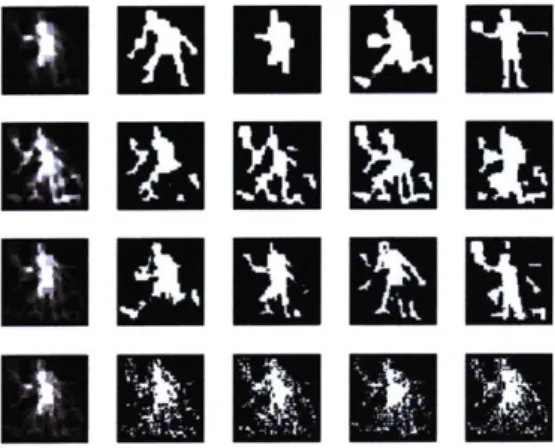
2-2 First line: max-margin parameters and resulting segmentation, second line: the mean of the perturbation parameters, the average segmenta-tion and the four images with the highest count. . . . . 75

2-3 Correlations between a reference pixel (white) and the rest, as captured by the covariance matrix of the perturbation distribution. We show a pixel that is always off (so no correlations) and two pixels that are activated on different poses. . . . . 76

2-4 The average segmentation and samples from four models, one per line: perturbation model where the perturbations have unrestricted vs. di-agonal covariance matrix and multivariate gaussian model with unre-stricted vs. diagonal covariance matrix. . . . . 76

2-5 Visual permutation learning: given a permuted sequence of images, the goal is to discover their underlying meaningful ordering (in this case, the order in which they appear in the original image). . . . . 78

2-6 The jigsaw puzzle solving architecture, same as Mena et al. [102]. The arrows indicate the computation flow: the input pieces are em-bedded independently via a convolutional model and used to produce unnormalized preference vectors over the output positions. The output permutation is obtained from the preference vectors via a maximum m atching algorithm . . . . . 80

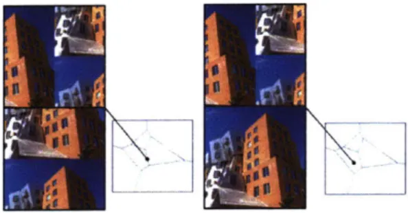
2-7 Combinatorial inverse optimization illustration. The top images are the scrambled inputs, while the bottom images are obtained by solving the inverse program, running a maximum matching algorithm on the solution, and applying the output permutation. On the left side, we used the inverse program formulation without a margin, which can lead to the optimal assignments being placed on the border between two inverse sets. When including a margin term, the solution is guaranteed to be placed inside the inverse set . . . . 84

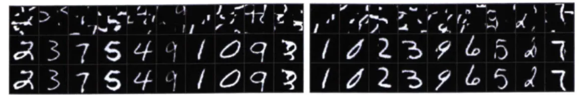
2-8 Model predictions, random samples. In each row pair, the top row indicates the shuffled input, and the bottom row indicates the predic-tion. We do not show the target since it is self explanatory. We show samples from the untrained model (left) and the trained model (right). 88

2-9 Unsolved samples at various iterations. NW: iteration 0 (random model), NE: iteration 25 (i.e. after seeing 2500 examples), SW: it-eration 50, SE: last model (after 10x540 itit-erations). In each row pair, the top row indicates the prediction, and the bottom row indicates the target. Note that in the unsolved examples, the model correctly builds a structure in the middle of the image, but it fails to capture the finer grained structure. The last group is shorter because there were only six misclassified examples in the validation set. . . . . 88

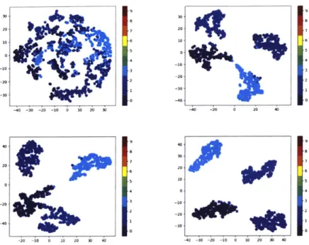
2-10 Matrix row embeddings colored by their target index. NW: iteration 0 (random model), NE: iteration 25 (i.e. after seeing 2500 examples), SW: iteration 50, SE: last model (after 10x540 iterations). This in-dicates that indeed the network learns to quickly cluster the patches according to their target location. . . . . 89

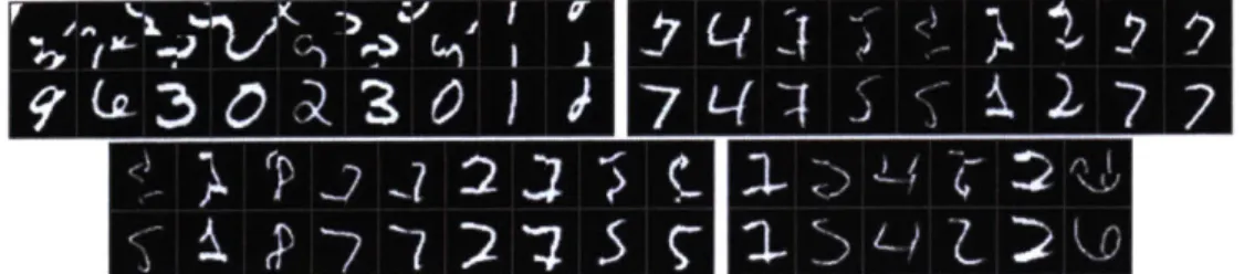
2-11 Solved examples on the MNIST-3 x 3 task. In the left group we show arbitrary samples from the validation set. In the right group we show examples where the accuracy is strictly smaller than 1. For each group, the top row shows the input (scrambled) pieces, the middle row shows the reconstructed image, and the bottom row shows the target recon-struction . . . . . 91

3-1 The Attend, Infer, Repeat (AIR) [36] encoder model. The input image

x is decomposed into a variable number of objects, each represented

through a location and a content variable. . . . . 100

3-2 The Attend, Infer, Repeat (AIR) [36] decoder model. Given a variable number of inputs, each corresponding to the location and content of an object, the model produces an image incorporating all the items. . 101

3-3 The Adaptive Computation Time approach

[52].

The model computes a preliminary halting probability estimate per node o-(Wh') (orange boxes) from the recurrent hidden state (blue boxes). Computation continues as long as the sum of estimated halting probabilities (dark grey progress bar) does not exceed (1 - c). The last halting probability estimate is set to the remaining total halting probability mass (rather than the extracted estimate from the state) and we indicate this via the dotted arrow. The existence probability per node can be extracted from the remaining total halting probability at each time step (light gray ). . . . . 103 3-4 Linearization of the hierarchical grouping of latent variables. The

bi-nary representation is used for topology prediction (with 1 indicating to continue generating children and a 0 indicating the end of the chil-dren list). The three shades of blue indicate the nodes corresponding to the same level of coarseness. . . . . 108 3-5 The neural network unit per tree node. The arrows indicate the flow of

information. Each orange box is an instance of a generator model. We denote by ppres, Pz the parameters of the distribution over the structure variable s and content variable z respectively, and by T the parameters of the attention model which indicate how the output of the current node should be placed on the canvas. . . . . 109 3-6 Accuracy on the training set at iterations 10, 000 (blue), 30, 000 (red),

200000 (magenta) as a function of the topology loss scale. Note that, due to reduced computational resources, we ran for further iterations only the models which performed best in the initial iterations. Evalu-ated across a single run per topology loss. . . . . 111 3-7 Training curves for a topology loss scale of 50 (left) and 60 (right),

3-8 Too small topology loss scale (left) and too high topology loss scale (right) with the inferred objects per time step highlighted. The extra small digit indicates the number of time steps inferred. Red / green

blue boxes indicate each time step (red = 1, green = 2, blue = 3). . . 113

3-9 Input (left) and reconstructions (right) with the inferred objects per time step highlighted. The extra small digit indicates the number of time steps inferred. Red / green / blue boxes indicate each time step (red = 1, green = 2, blue = 3). Note that in the last column, the blue and green area overlap. . . . . 113

3-10 The plot shows the accuracy (in terms of the number of time steps vs. actual number of objects) as a function of the topology loss scale used for training. Note that in this experiment, the each image contains at least one object, and we force the model to do the same. At the highest scale, the model predicts a single time step, resulting in 0.5 accuracy. At the lowest scale, the model uses all the available time steps, resulting in 0 accuracy. The images show samples from the model: example reconstruction with a maximum number of time steps (middle) and samples from the decoder model per time step (right). . 114

4-1 Node-based generation as in You et al [1621. In the figure, the new node per time step is shown in green, and the previously generated nodes in gray. The model computes existence probabilities for each candidate edge between the new node and previous nodes, and these are illustrated with blue lines of varying width. The node-level prediction is a binary adjacency vector w.r.t. the previous nodes (most recent nodes first), which is used to update the evolving structure (right graphs). . 130

4-2 The figure illustrates the effect of the node-level output size All on a sequence of generated nodes: when M = V I-1 a new node can connect to any previously generated node, when M = 2, the new node can only connect to its two predecessors, enabling improved computational performance. Previous work [162] uses BFS orderings and fixes M to match the maximum BFS queue size. Instead, we ask whether we can fix M and search for predictable (not necessarily BFS) orderings. . . 131 4-3 Sampling from the approximate posterior. The prior probabilities

(il-lustrated by blue lines of varying width in the top-left graph) are renor-malized over the feasible candidates to produce the approximate pos-terior probabilities (blue lines of varying width in the middle graph). The target (bottom-left graph) is a cycle, so the new node can only be attached to the left or the right ends. . . . . 132 4-4 Feasibility test. When restricted to the completed nodes (A), the

prob-lem corresponds to an induced subgraph isomorphism probprob-lem. How-ever, our problem includes an incomplete node (B). . . . 136 4-5 Polynomially solvable special cases. . . . 137 4-6 BFS orderings consistent with the target graph (left). The two node

orderings shown (middle and right illustrations) require M > 2 and M > 4, respectively. . . . 138 4-7 Baseline samples from a model learned on the grid dataset. We display

samples selected by iterating over the dataset graph sizes and, for each graph size, selecting a generated graph whose size is closest. The left group (4x4) shows the graphs corresponding to the smallest 16 sizes, while the right group shows the graphs corresponding to the largest 16 sizes. . . . .. . .. . . . . 152 4-8 Samples obtained from training with the approximate posterior, on the

grid-small dataset, obtained across two train-test seeds. . . . . 153 A-1 The Attend, Infer, Repeat (AIR) Model Equations. . . . .1 158

List of Tables

2.1 Various accuracy measures computed for our trained model on MNIST-3 x MNIST-3, and shown side-by-side with the results extracted from Mena et al [102]. We evaluated the model across two runs and note that the difference between results was less than 0.01, so we are not reporting the standard deviation in this table. . . . . 91

3.1 Accuracy of detecting the number of objects in the input image. We report the mean across training runs with the standard deviation in the parentheses. In the Soft-AIR case, we report the results obtained for a topology scale equal to 50, since it performed the best in our analysis from the previous section. However, more runs, with a higher frequency between topology scale steps, might uncover better-performing models. 113

4.1 Graph datasets statistics. The last column indicates the choices con-sidered for the output size M. In the experiments below, we will specify the chosen M together with the dataset name (e.g. grid-small-15 to indicate that we use the grid-small dataset with M = 15). . . . . 141

4.2 Baseline results on the MMD-based evaluation metrics proposed in the cited work [162J. We evaluate these metrics to verify that the trained models perform similarly to those in the cited work. . . . . 150

4.3 Baseline results on the likelihood metrics discussed in sections 4.6.2.1 - 4.6.2.3. We report the results at the last epoch (3000). Note that, for datasets such as grid-small, due to the small number of examples, the difference in graph length statistics across training and test sets reflects in the average NLL scores. While averaging over multiple splits could alleviate the issue, we also point the reader to PPL scores, which are averaged across edge predictions and are less sensitive to varying graph lengths. . . . .

... ...151

4.4 Baseline results on the likelihood metrics discussed in sections 4.6.2.1 - 4.6.2.3. We report the results at the last epoch (3000). Note that the improved results when evaluating on the canonical ordering for the k-path-small datasets indicate that the model learns a preference for that ordering, even when trained across all sequences. . . . . 152

1

Introduction

Contents

1.1 Motivation ... ... 21 1.2 Contribution .. .. .... ... . . .. .. ... ... .. 26

1.1

Motivation

Structured prediction problems are prevalent in computer vision, natural language, speech processing, bioinformatics, and many others fields. Whether the goal is com-puting image segmentations, uncovering the hierarchical structure of natural lan-guage, transcribing a speech, or generating protein structures, the models involve high-order dependencies between the output variables. These dependencies make structure prediction challenging.

Graphical models. Structured potential functions that are used to model the de-pendencies in graphical models must make strong assumptions to enable efficient

in-ference. There are two fundamental inference problems:

1. Computing a single, best assignment of the structured output variables given the input (MAP inference), and

2. Extracting one of the many possible outputs according to their probability of realization (sampling).

Unfortunately, in both cases, the resulting inference calculations can become compu-tationally intractable whenever the structured potential function includes high-order terms. Sampling is particularly challenging, due to the requirement of summing over all the terms in order to obtain calibrated probability values. This task often remains computationally intractable even when computing the best assignment is not (see, for instance, the bipartite matching problem [146]). A critical challenge in this setting is building models which are powerful, yet easy to sample from.

One-shot decoding with neural networks. In recent years, neural network-based approaches have demonstrated that models which predict each output variable inde-pendently of the others, but which rely on rich multi-layer features, can provide state of the art results for structured prediction tasks, including image segmentation [93], pose detection [143], and many other applications. These one-shot decoding models consist of parametrized feed-forward mappings from input to outputs and can be successfully trained for tasks where the goal is to compute single assignments, cor-responding to performing MAP inference. Furthermore, unlike structured potential functions, these models make fewer or no assumptions about the (structure of the) problem, rendering them more flexible. In the context of generative models, however, early applications of feed-forward networks, such as Deep Belief Networks (DBNs)

[63],

continued to involve intractable sampling steps, requiring the use of Gibbs sam-pling [63, 129].

Implicit models. Fortunately, both structured potential functions and feed-forward neural networks can increase modeling power and sampling efficiency through the use

of implicit distributions. Specifically, recent approaches have developed lightweight structured prediction models by taking advantage of efficient computational primi-tives designed for computing single assignments, such as MAP solvers, or feed-forward neural network mappings. For instance, perturbation models [23, 26] define proba-bilistic models via efficient deterministic optimizers with randomized parameters; the variational auto-encoder (VAE) framework [16] maps simple priors to distributions over text or images; the generative adversarial network (GAN) framework [8] simi-larly maps generic noise to images. The joint strategy is mapping samples from simple distributions into samples from highly structured distributions. Whenever sampling is challenging to perform, or it requires restrictive assumptions on the structure of the models, implicit distributions provide a promising alternative.

Nevertheless, when predicting all the outputs at once, neural network models may fail to capture critical dependency structure, even when relying on stochastic latent variables for increased modeling power. In image generation, for instance, when assuming that individual pixels are independent of each other conditioned on the input, neural network models may miss small-scale features such as textures or sharp edges, resulting in decreased quality of image samples and reduced log-likelihood

[55].

Furthermore, when predicting all output variables at once, neural network models may not capture the expected global constraints, such as connectivity or tour structure, one having to resort to post-processing heuristics to enforce the desired properties [109, 134]. For instance, in previous work on graph generation [134], while all the training examples consisted of connected graphs, the authors imposed connectivity at test time by selecting the maximum spanning tree over the predicted adjacency matrix, creating a discrepancy between the manner in which inference is performed at training time vs. test time.

Sequential decoding. Sequential models, which incorporate dependencies between outputs more explicitly have been successful at modeling sequences [138] as well as more complex structures [149, 111]. In many cases, they enable efficient maximum likelihood training for even highly complex models [111] and facilitate the hard-coding

04

GANs 0 _{Perturbation Models}

Sequlential Decoding Models DBNs 0

A-0 1 Graphical Models 00 0.5 0.5 1 0

Sampling Complexity Model Expressivity

Figure 1-1: Illustration of various models along the axes of interest, namely sam-pling complexity, MAP complexity, and model expressivity. In placing the points, we only distinguished between high/low quantities (e.g. whenever sampling is easy, the corresponding point is located close to 0, and whenever sampling is computationally challenging, the corresponding point is placed close to 1, with the actual values being selected arbitrarily). The corner highlighted in gray shows the broad focus of the thesis: expressive models that are nevertheless easy sample from. In particular, we explore perturbation models and sequential decoding models, shown in blue.

of global constraints by rejecting infeasible choices early

[14].

Concerning the com-plexity of inference, sequential decoding models enable efficient ancestral sampling, but computing a maximizing assignment is challenging, typically being performed via greedy methods, and beam search [158].

The models described so far vary along the following significant axes: the complex-ity of performing sampling, the complexcomplex-ity of computing the maximum-a-posteriori (MAP) assignment, and the modeling power (expressivity) of the model. We high-light the axes in Figure 1-1. For instance, graphical models, using structured potential functions, are generally challenging to sample from, even when MAP inference can be performed efficiently. Sequential decoding models, perturbation models, as well as one-shot decoding models defined via implicit distributions (VAEs, GANs), enable efficient sampling while computing the MAP assignment becomes challenging.

Figure 1-1), and we approach the task from two broad perspectives: defining models via structured potential functions, and via sequential neural network-based decoders. In the former case, we explored implicit distributions defined via optimization of ran-domized structured potential functions (perturbation models). Designed explicitly for efficient sampling, perturbation models are strong candidates for building generative models over structures, and the leading open questions pertain to

9 Understanding the properties of the perturbation models,

e Developing practical learning algorithms for learning perturbation models.

In the latter case, we explore building sequential models for structure decoding, and the main challenges to address are

o Designing appropriate sequentializations,

o Dealing with the discreteness of intermediate structure representations,

which we describe below.

The sequentialization of a complex structure refers to its conversion into a sequence of more straightforward choices, such as predicting a tour by enumerating the traversed nodes or predicting a graph by enumerating its edges1. Sequentialization can be achieved in a variety of ways, as can be seen by the multiple ways to describe a tree, including via its set of edges, a depth-first traversal or a breadth-first traversal. We lack a principled understanding of how to choose one approach versus another. Furthermore, previous work on modeling groups of items [148] showed that a poorly chosen sequentialization could hinder performance. For instance, when modeling a star-like graphical model as a sequence, predicting the structure by processing the center (parent) element first was empirically shown to be easier to optimize than the equivalent learning problems where leaf nodes are processed before the parent. The cited result highlights that, in some problems, the chosen ordering of output variables 'It should not be confused with the term arising in computing theory where it refers to the process of converting a parallel program into a sequential one (e.g., [18]).

is essential in producing an easy to optimize sequential model.

The second key challenge in using sequential models for structure prediction concerns the presence of discrete intermediate representations. Dealing with discrete latent variables is challenging because the resulting objective function is non-differentiable

and one cannot apply the back-propagation algorithm directly. Instead, one must use gradient estimators such as the score function estimator

[157],

or replace the discrete choices with continuous analogs [52, 70, 96], or bypass the issue by providing addi-tional supervision when applicable [4]. Typically, the issue arises when the discrete structure is latent, whether modeled via one-shot decoding or sequential approaches, in problems such as natural language modeling via latent tree representations [156], scene generation with a latent number of objects

[36],

or discriminator-based learning of discrete structures [65]. However, even when dealing with observed structured vari-ables, a sequential generation process produces intermediate discrete varivari-ables, such as node indices when predicting tours for solving the Traveling Salesman Problem [14] or binary edge predictions for performing graph generation [162]. Step-level supervi-sion enables the use of teacher forcing [87], however, in many problems of interest, such as graph generation, an appropriate node-level supervision scoring function is not readily available [134].

The next section will discuss the scenarios we consider in more detail.

1.2

Contribution

We aim to predict discrete structures, such as alignments, sequences, graphs, which are amenable to modeling through optimization methods and sequential models. In the former case, we explored implicit distributions defined via optimization of ran-domized structured potential functions. In the latter case, we explored learning se-quential models via maximum likelihood training with step-wise supervision and via continuous relaxations of the intermediate discrete variables. We tackled the resulting

challenges in the context of three scenarios:

* Perturbation Models. In this context, we address the challenges described in the previous section, namely characterizing and learning perturbation models. We present theoretical results showing that, in contrast to the more established Gibbs models, low-order potential functions, after undergoing randomization and maximization, lead to high-order dependencies in the induced distribu-tions. Furthermore, while conditioning in Gibbs' distributions is straightfor-ward, conditioning in perturbation models is typically not, but we theoretically characterize cases where the straightforward approach produces the correct re-sults. Finally, we introduce a new algorithm for learning perturbation models via Inverse Optimization. We illustrate both the induced dependencies and the inverse optimization approach empirically, in learning problems inspired by computer vision tasks, such as binary image modeling, and visual permutation learning.

" Scene Understanding. In dealing with discrete latent variables, the main approaches consist of using gradient estimators and designing continuous re-laxations. We discuss these solutions in the context of unsupervised scene un-derstanding with generative models. In particular, we asked whether using continuous relaxations of the binary latent variables involved in counting the objects in an image also enables discovering the objects in an unsupervised fash-ion. To this end, we proposed and investigated a scene understanding model based on the Adaptive Computation Time (ACT)

[52]

approach which achieves the desired result.

" Iterative Graph Generation. In the context of sequential graph generation, we propose a variational lower-bound to the maximum likelihood objective. The proposed approximate posterior distribution renormalizes the prior distribution over local predictions which are plausible for the target graph. For instance, the local predictions may be binary values indicating the presence or absence

of an edge indexed by the given time step, for a canonical edge indexing chosen a-priori. The plausibility of each local prediction is assessed by solving a com-binatorial optimization problem, and we discuss relevant approaches, including an induced sub-graph isomorphism-based algorithm for the generic graph gener-ation case, and a polynomial algorithm for the special case of graph genergener-ation resulting from solving graph clustering tasks. In this thesis, we focused on the generic case, and we investigated the approximate posterior's relevance on synthetic graph datasets.

2

Generating Discrete Structures via

Perturbation Models

Contents

2.1 Introduction . . . . 30 2.2 Related Work . . . . 33 2.3 Perturbation Models . . . . 34 2.4 Implicit Distributions . . . . 36 2.5 Characterization of Perturbation Models . . . . 38 2.5.1 Expressive Power of Perturbation Models . . . . 38 2.5.2 Higher Order Dependencies . . . . 39 2.5.3 Markov Properties and Perturbation Models . . . . 41 2.5.3.1 Tree-Structured Perturbation Models . . . . 42 2.5.4 Conditional Distributions . . . . 44 2.5.4.1 Max-marginals . . . . 46 2.5.4.2 Conditional Independence . . . . 47 2.5.5 Perturbation Models and Stability . . . . 53 2.6 Learning Perturbation Models . . . . 56 2.6.1 Structured Potential Function Modeling . . . . 57

2.6.2 Learning Objective . . . . 59 2.6.2.1 Hard-EM . . . . 60 2.6.3 Inverse Optimization . . . . 62 2.6.3.1 Complementary Slackness . . . . 64 2.6.3.2 Margin-Augmented Inverse Optimization . . . . . 65 2.6.3.3 Exam ples . . . . 68 2.6.3.4 Lim itations . . . . 73 2.7 Empirical Results . . . . 74 2.7.1 Image Segmentation . . . . 75 2.7.2 Visual Permutation Learning . . . . 77 2.7.2.1 Problem Formulation . . . . 79 2.7.2.2 Model Architecture . . . . 80 2.7.2.3 Implementation Details for Inverse Optimization . 82 2.7.2.4 Experimental Setup . . . . 85 2.7.2.5 Understanding Inverse Optimization . . . . 88 2.7.2.6 Comparison to Previous Work . . . . 90 2.7.2.7 Potential Extensions . . . . 92 2.8 D iscussion . . . . 93

2.1

Introduction

In applications that involve structured objects, such as object boundaries, textual descriptions, or speech utterances, the key problem is finding expressive yet tractable models. In graphical model approaches, the likely assignments are guided by potential functions over subsets of variables. The feasibility of inference is typically linked to the structure of the potential function and the tradeoff is between rich, faithful models defined on complex potential functions on one hand, and limited but manageable models on the other.

For instance, in natural language parsing, the goal is to return a dependency tree where arcs encode dependency relations, such as between a predicate and its subject.

Whenever the interactions are of high order, computing the dependency tree corre-sponds to an NP-hard combinatorial optimization problem

[101],

but when resorting to tractable formulations by limiting the type of interactions, the expressive power of the model is limited. In general, most realistic models for natural language pars-ing [83], speech recognition [120] or image segmentation/ captionpars-ing [110, 37] involve interactions between distant words in the sequence or large pixel neighborhoods.

Typical probabilistic models defined on structured potential functions make use of the Gibbs' distribution and its properties. Specifically, the structure of the potential function can be encoded as a graph that specifies conditional independencies (Markov properties) among the variables: two sets of vertices in the graph are conditionally independent when they are separated by observed vertices (e.g., [151, 81]). These assumptions are central for designing efficient exact or approximate inference tech-niques. Successful methods exploiting them include belief propagation [117], Gibbs sampling [48], Metropolis-Hastings [59] or Swendsen-Wang [152]. In specific cases one can sample efficiently from a Markov random field model by constructing a rapidly mixing Markov chain (cf. [71, 72, 67]). Such approaches do not extend to many practical cases where the values of the variables are strongly guided by both data (high signal) and prior knowledge (high coupling). Indeed, sampling in high-signal high-coupling regime is known to be provably hard [71, 49].

Finding a single most likely assignment (MAP) structure can be considerably easier than summing over the values of variables or drawing an unbiased sample. Substan-tial effort has gone into developing algorithms for recovering MAP assignments, either based on specific structural restrictions such as super-modularity [82] or by devising linear programming relaxations and successively refining them [135, 154]. Further-more, even when computing the MAP is provably hard, approximate techniques, such as loopy belief propagation [105], tree reweighed message passing [150], local search algorithms [164] or convex relaxations [84] are often successful in recovering the optimal solutions [83].

In recent years, MAP inference has been combined with randomization to define new classes of probability models that are easy to sample from [116, 140, 60, 61, 113, 981. Each sample from these perturbation models involve randomization of Gibbs' poten-tials and finding the corresponding maximizing assignment. The models are shown to provide unbiased samples from the Gibbs distribution when perturbations are inde-pendent across assignments [116, 140] and have been applied to several applications where the underlying combinatorial problem is easy to optimize, but difficult to sam-ple from, including boundary annotation [98] and image partitioning [77], but having a full account of the properties and power of perturbation models remains an open problem.

In this chapter, we describe and extend our work [45, 461 on understanding and exploiting the expressive power of perturbation models. Specifically, the properties of the induced distribution are heavily governed by randomization. In contrast to Gibbs' distributions, low order potentials, after undergoing randomization and maximization, lead to high order dependencies in the induced distributions. Furthermore, while conditioning in Gibbs' distributions is straightforward, conditioning in perturbation models implies restricting the randomizations to a non-trivial set and performing this efficiently is still an open problem.

Finally, we explore the interplay between learning algorithms and tractability of infer-ence procedures on complex potential functions. We describe dependent perturbations as a modeling tool for learning models which lead to tractable inference. Perturbation models are latent variable models and we learn distributions over perturbations using a hard-EM approach, illustrating on a synthetic dataset how the modeling power is split between the latent space and the optimization step.

In cases where the optimization step can be phrased as a linear program with a small number of constraints, we use an inverse convex program in the E-step to confine the randomization to the parameter polytope responsible for generating the observed answer. In previous work [45], we illustrated the approach on an image matching task.

In this chapter, we implement the inverse optimization-based learning algorithm in the context of a recently proposed Visual Permutation Learning task [29]. The challenge we encounter, also noted in Tarlow et al.

[140],

is that the element in the inverse set returned by the inverse program might be close to the border, such that the learning algorithm places probability mass both inside and outside the inverse set. To this end, we adjust the inverse program constraints to include a linear margin term.

2.2

Related Work

The Gibbs distribution plays a key role in many areas of computer science, statistics and physics. To learn more about its roles in machine learning we refer the interested reader to [81, 151]. The Gibbs distribution as well as its Markov properties can be realized from the statistics of high dimensional random MAP perturbations with the Gumbel distribution (see Theorem 1), [116, 140, 60, 61]. For comprehensive introduction to extreme value statistics we refer the reader to [85].

Recent works [115, 116, 140] explore different aspects of low dimensional MAP per-turbation models. Papandreou et al. [115] describe sampling from the Gaussian distribution with random Gaussian perturbations. Later , they show empirically that MAP predictors with low dimensional perturbations share similar statistics as the Gibbs distribution. In our work we investigate dependencies introduced by such probability models. Specifically, we present non-i.i.d. low dimensional random pertur-bations that reconstitute Markov properties of tree structured Markov random fields. We also show that independent low dimensional perturbations involve long-range in-teractions. Tarlow et al. [140] propose several techniques for learning perturbation models, including hard-EM. In contrast, we focus on understanding the structure of the induced distribution and our learning approach is different. We use dual LPs in our hard-EM approach so as to obtain compact representations of the inverse poly-tope when possible, while Tarlow et. al [33] focus on cutting plane approaches. When using cutting plane approaches for only a couple of iterations, the hard-EM estimates

often fall outside the inverse polytope. Our dual LP approach alleviates this problem and in our experiments almost all estimates fall within the inverse polytope.

Our experiments show that we are able to sample from the modes of the distribution. Alternatively, one may use the M-best approach and its diverse-versions to recover such modes [161, 42, 12, 103, 13, 57]. Finding the M-best carries a computational effort which extends beyond our learning approach whose complexity is as a 1-best solver. Alternatively, one may sample from determinantal point processes to retrieve modes of distributions [86]. This approach concerns problems that can be described by determinants while our approach is based on MRF potentials.

2.3

Perturbation Models

We are concerned with modeling distributions over structured objects x

E X, such as

image segmentations and key-point matchings, where X = X x -- - x X, is a discrete product space. We score the possible assignments via a real valued potential function 0(x) 0(xi, ... , x,), where excluded configurations are implicitly encoded by setting

0(x) = -o whenever x 1 dom(0).

For instance, a foreground-background segmentation over an image of size n x m can be encoded by x (xij)ic[n,JE[m] E {0, 1}nxm, where xij = 1 denotes a foreground pixel at position (i, i). If we want to explicitly encode that there always exists a foreground object, we can enforce that 0(x) = -oC whenever xij = 0 for all i C [n],

j

E [m]. If we want to further encod that the foreground object is contiguous, we may enforce that 0(x) = -o whenever the graph G = (V, E), with V = {(i, j)|lij = 1} and Vu = (ui, uj), v = (vi, vj), E V, Eu,v = 1 iff the pixels positioned at (ui, 'a) and (vi, vj) are adjacent, has more than one connected component.

Since dealing with arbitrary scoring functions is computationally intractable, 0(x) is typically defined as a sum of local potentials 0(x) = Ea A0(x), where a denotes a small subset of variables (factor) and A denotes the set of all such factors. In

the image segmentation case, for an image of size n x n pixels, A may include local neighborhoods of the form {(i + d,, j + d) Ii, j

c

{1 ... n}, dX, dy E {+1, 0, -1}}, as well as global factors for encoding excluded configurations as discussed above. In the following, we will often skip specifying A and write 0(x) =

Za

0, (x) for simplicity. Traditionally, the potentials are mapped to the probability scale via the Gibbs' dis-tribution:

p (xi .. ,1 ) = Z 6 , ..., x.,,a) (2.1)

Distributions defined in this manner have a number of desirable properties. For instance, the maximum-a-posteriory (MAP) prediction corresponds to the highest scoring assignment i = arg maxx 0(x), the set of conditional dependencies can be read from the structure of the potential function, and the model can be easily extended to handle partially observed data. Unfortunately, such distributions are challenging to learn and sample from, depending on how the potential function decomposes.

Our approach is based on randomizing potentials in Gibbs' distributions. We add a random function -y : X -+ R to the potential function and draw samples by solving

the resulting MAP prediction problem:

X* arg max{0() + 7(x)}. (2.2)

The distribution induced by the samples is given by

'P() P[ E arg max{0(x) + y(x)}] (2.3)

and its properties are heavily dependent on the nature of randomization.

The simplest approach to designing the perturbation function -y is to associate an i.i.d. random variable -y(x) for each x C X. The following result characterizes the

Specifically, due to the max-stability property of the Gumbel distribution, one can preserve the Markov properties of the Gibbs model. However, each realization x* in this setup requires an independent draw of -y(x), x E X, i.e., a high dimensional randomization.

Theorem 1

[56]

Let X be finite and let

{y(x),

x

C

X} be a collection of i.i.d. zero mean Gumbel distributed random variables, whose cumulative distribution functions is F(t) = exp(- exp(-(t + c))) and c ~ 0.5772 is the Euler-Mascheroni constant.

Then

- 1

P [i

c

arg max{0(x) + (() exp(0())) (2.4)

xEX _{. 2.0)}

However, this construction requires that for every sample d we must instantiate 1XI random variables (-y(x))xex, which is not feasible in practice. Since perturbation models are useful only if they can be succinctly parametrized, our focus is on investi-gating low-dimensional perturbations which have the same structure as the potential function:

P,[ Earg max (0( a( ) + - ('Xa)) (2.5)

In this case, each sample requires instantiating -ya(x0) for each a and each assignment

Xa, which is typically a much smaller set. Finally, since the noise function shares the structure of the potential function, the optimization algorithms designed for the origi-nal potential function remain applicable. We will often refer to the new (randomized) potential function as 0(x) = E 0,(x,), where 0a(x,) = 0a('a) + Ya (Xa).

2.4

Implicit Distributions

Perturbation models can be viewed as a special case of implicit distributions [68]. In particular, they both map samples from simple distributions into samples from highly

*ON-* ...

---Figure 2-1: Broad structure of implicit distributions: samples from a generic distri-bution are mapped through a complex mapping to realize the distridistri-bution of interest. The black box mapping can be realized via an optimization solver (left) or a neural network (right).

structured distributions. The mapping involves one of the following two components (Figure 2-1 graphically depicts this connection):

* A nonlinear mapping;

" An (efficient) optimization solver.

For instance, perturbation models [116, 141] define probabilistic models via efficient deterministic optimizers with randomized parameters, whereas [51] map generic Gaus-sian priors to distributions over text or images via rich neural network decoders. Neural networks provide efficient, rich and flexible feature mappings and are therefore the perfect candidate for morphing simple distributions into complex ones. Neural networks typically entail many layers of non-linear, non-invertible differentiable trans-formations thereby inducing highly complex dependencies among variables, even when the output (prediction) layer is completely unstructured. The associated challenges typically relate to carefully designing the mapping to enable efficient training via gradient descent.

On the other hand, in the optimization case, the mapping from input to target vari-ables is defined via a potential function over subsets of varivari-ables which captures their interactions. Such interactions allow defining complex scoring function over the pos-sible assignments as well as discrete structural properties, such as tree structured assignments, matchings, paths, and so on, which are difficult to enforce in neural

network settings as we discuss later in this thesis. In this chapter, we choose the optimization approach and in the following section we discuss the properties of the induced distribution as they relate to the choice of optimization solver.

2.5

Characterization of Perturbation Models

2.5.1

Expressive Power of Perturbation Models

Perturbation models were originally introduced as a way to approximate intractable Gibbs' distributions. In this chapter, we use perturbation models as a modeling tool, seeking to understand their properties, and how to estimate them from data.

The idea of specifying distributions over combinatorial objects by linking random-ization and combinatorial optimrandom-ization is not inherently limiting. At one extreme, the randomization may correspond to samples from the target distribution itself. Of course, the combination is advantageous only when both the randomization and the associated combinatorial problem are tractable. To this end, we focus on random-izing potentials in Gibbs' distributions whose MAP assignment can be obtained in polynomial time. The randomization we introduce will therefore have to respect how the potential functions decompose. For example, randomization of 0(x) = E 0a(x)

should only directly affect individual terms 0,(x).

One of the key questions we address is how the resulting perturbation models dif-fer from the associated Gibbs' models that they are based on. Gibbs' distributions are naturally understood in terms of Markov properties. Will these carry over to perturbation models as well? We will show that in contrast to Gibbs' distributions, low order potentials, after undergoing randomization and maximization, lead to high order dependencies in the induced distributions. Such induced dependences can be viewed as additional modeling power and specifically exploited and learned from data. Markov properties can be enforced in special cases such as with tailored perturbations

in tree structured models, if desired.

Perturbation models yield simple mechanisms for drawing unbiased samples but they are cumbersome with respect to conditioning. Indeed, "plug-in" conditioning natural in Gibbs' distributions does not carry over to perturbation models. Conditioning requires care, restricting the randomization such that the setting of the observed variables are indeed obtained as part of maximizing assignments. We show how this can be done in simple examples.

2.5.2

Higher Order Dependencies

In this section, we show that perturbation models defined via low dimensional ran-domizations do not follow the Markov-type dependencies inherent in Gibbs distri-butions. We focus on perturbation models with tree structured potential functions and edge-based randomization, but the results can be generalized to more complex graphs.

The following theorem shows that when i.i.d. perturbations follow the edge structure of the potential function, we are able to capture dependencies above and beyond the initial structure.

Theorem 2 Consider chain model with three variables (xI, X2, X3), xi e {0, 1, and

potential

function

0(x) = 012(x1, X2) + 023 (X2, 3). Then there exist local potential

functions 012,023 and i.i.d. perturbation distributions over {'ij (xi, x)}} indexed by

(i, j) E {(1, 2), (2, 3)}, xi, x3 E {0, 1} s.t. x1 LX 3X2 in the induced model specified in eq. (2.5).

Proof 1 Let F(da) be defined as

F(z) = sE arg max{0(x) + Y(x)}} (2.6)

assignment i, is included in the complete assignment returned by the arg max at the corresponding positions given by a.

Similarly, for all subsets a, C {1,... , n}, let

= {y: Earg max {0(x)+ Y(x)}} (2.7)

be the set of perturbation assignments for which 1: is optimal if we plug-in values 29. We illustrate that x, 1 3 |2 need not hold. To this end, consider probabilities:

P (i| 122) =Py (F (: i 12)|1 r(i2)) , for Z E {1, 3} (2.8)

Note that the set F(J11-12) is governed by the constraint 012(1:1, x2) + 7Y12(-J1,-':2) ->

maxx1{012(xi, 1:2) + 7Y12(XI, i2)} and similarly, F(i3j: 2) is governed by an analogous

constraint on Y23. P(1:2), in contrast, involves inequalities that couple all the

per-turbation variables together: maxx1{012(Xi, 1:2) + 712(x1, x2)} + maxX3{023(1: 2, X3) +

723(i2, X3)} > maxxf{0(x) + -712(X1, X2) + 'y23(X2, X3)}. Since in general these

con-straints cannot be decomposed as (-Y12, 723), the set is not a product space.

Consider the following example, where xi C {0, 1} and 012(1, 1) = 1.9, 012(0, 0) = 1.2,

012(0, 1) =1.1, 012(1, 0) = 0 and 023(a, b) = 012(b, a), Va, b C {,1} . For 2 =1, F (12)

includes the constraint max{1.9+71 2(1, 1), 1.1+-Y12(0, 1)}+max{1.9 +7 2 3(1, 1), 1.1+

723(1, 0)} ;> max{1.2 + 712(0, 0), 712(1, 0)} + max{1.2 + Y23(0, 0), 123(0, 1)}. We argue that there exist i.i.d. perturbation distributions over (712,723) for which the

con-straint couples the two variables. In particular, if 112(XI, 2) U{-1, 1} V(xi, 2) C

{0, 1}2, 723(X2, 3) ~ U{--1, 1} V(x2, 3) C {0, 1}2 and U is the uniform distribution,

then for 7yij = (745(1 1) 135(0, 1) 7 i(0 0), yij(1, 0)), the configurations (712, 123) E

{((1, 1, -1, 1), (-1, 1, 1,1)), ((1, 1, -1, 1), (1, 1, -1, 1)), ((-1, 1, 1,1), (1, 1, -1, 1)) }, are

in F(i2), but ((-1, 1,1, 1), (-1, 1, 1, 1)) is not, thus it cannot be a product space in

this case.