HAL Id: halshs-01719835
https://halshs.archives-ouvertes.fr/halshs-01719835v2
Preprint submitted on 27 Jan 2021
HAL is a multi-disciplinary open access archive for the deposit and dissemination of sci-entific research documents, whether they are pub-lished or not. The documents may come from teaching and research institutions in France or abroad, or from public or private research centers.
L’archive ouverte pluridisciplinaire HAL, est destinée au dépôt et à la diffusion de documents scientifiques de niveau recherche, publiés ou non, émanant des établissements d’enseignement et de recherche français ou étrangers, des laboratoires publics ou privés.
Inference on time-invariant variables using panel data: a
pretest estimator
Jean-Bernard Chatelain, Kirsten Ralf
To cite this version:
Jean-Bernard Chatelain, Kirsten Ralf. Inference on time-invariant variables using panel data: a pretest estimator. 2021. �halshs-01719835v2�
WORKING PAPER N° 2018 – 07
Inference on time-invariant variables
using panel data:A pretest estimator
Jean-Bernard Chatelain
Kirsten Ralf
JEL Codes: C01, C22, C23.
Keywords: Time-invariant variables, panel data, pretest estimator, instrumental
vari- ables, Mundlak estimator, Hausman-Taylor estimator.
Inference on time-invariant variables using panel
data: A pretest estimator
Jean-Bernard Chatelainyand Kirsten Ralfz
January 26, 2021
Abstract
For static panel data models that include endogenous time-invariant variables corre-lated with individual e¤ects, exogenous averages over time of time-varying variables can be internal instruments. To pretest their exogeneity, we …rst estimate a random e¤ects model that includes all averages over time of time-varying variables (Mundlak, 1978; Kr-ishnakumar, 2006). Internal instruments are then selected if their parameter is statistically di¤erent from zero (Mundlak, 1978; Hausman and Taylor, 1981). Finally, we estimate a Hausman-Taylor (1981) model using these internal instruments. We then evaluate the bi-ases of currently used alternative estimators in a Monte-Carlo simulation: repeated between, ordinary least squares, two-stage restricted between, Oaxaca-Geisler estimator, …xed e¤ect vector decomposition, and random e¤ects (restricted generalized least squares).
JEL classi…cation numbers: C01, C22, C23.
Keywords: Time-invariant variables, panel data, pretest estimator, instrumental vari-ables, Mundlak estimator, Hausman-Taylor estimator.
1
Introduction
Panel data have a time-series and a cross-sectional dimension, but in some studies one or several relevant explanatory variables are time-invariant. Examples of key time-invariant variables are geographical distance for cross-country data in gravity models of foreign trade and foreign direct investments (Serlenga and Shin, 2007); years of schooling, gender, and race when testing Mincer’s wage equation using survey data (Hausman and Taylor, 1981); colonial, legal, or political systems; international con‡icts; institutional and governance indicators; and initial gross domestic product per capita when testing the convergence of incomes in growth regressions. These variables are often highly relevant and have a high expected correlation with a cross-sectional and time-varying dependent variable in the cross-cross-sectional dimension.
For static panel data models that include endogenous time-invariant variables correlated with individual e¤ects, exogenous averages over time of time-varying variables can be internal instruments. If the number of exogenous internal instruments is at least equal to the number of endogenous time-invariant variables, Hausman and Taylor’s (1981) estimator can be applied (for example, Goh and Tham, 2013; Bouvatier, 2014). This estimator assumes that the practitioner knows which averages over time of time-varying explanatory variables are not correlated with individual e¤ects.
Acknowledgements: We thank two anonymous referees for very helpful comments. We thank William Greene for helpful comments on a previous draft of this paper, see also Greene (2012), section 11.4.5. This paper is forthcoming in Economic Modelling.
yParis School of Economics, Université Paris I Pantheon Sorbonne, 48 Boulevard Jourdan, 75014 Paris,
zESCE International Business School, INSEEC U Research Center, 10 rue Sextius Michel, 75015 Paris,
However, practitioners rarely know whether a given time-varying explanatory variable is not correlated with individual random e¤ects. Without a pretest for the exogeneity of internal in-struments, the Hausman-Taylor estimator faces potential endogeneity bias by wrongly assuming that all internal instruments are exogenous.
Practitioners may also have too many sets of internal instruments available. For example, Greene (2012, Chapter 11) evaluates the returns to schooling using Mincer’s wage equation. The unique endogenous time-invariant variable (g2 = 1) is each individual’s years of education. The baseline equation includes k = 9 time-varying explanatory variables. Their average over time allows up to k = 9 internal instruments for the returns to schooling for the Hausman-Taylor estimate. Without a pretest for selecting which subset of 1 k1 of internal instruments includes variables that are not correlated with individual e¤ects, the researcher is left with too many choices of instruments sets. When varying the sets of internal instruments, there are no fewer than
i=kP1=9
i=g2=1
9
i = 2
9 1 = 511 Hausman-Taylor estimates of the returns to schooling.
Therefore, this paper proposes an instrument selection procedure using Hausman (1978) pretests of the endogeneity of each time-varying regressor. The practitioner computes the aver-age over time of all time-varying variables. In the …rst step, he runs a random e¤ects estimator that includes all time-varying variables, all time-invariant variables, and, most importantly, all averages over time of all time-varying variables (Mundlak, 1978; Krishnakumar’s (2006) esti-mator). The practitioner selects as internal instruments the subset of 0 k1 k averages over time of time-varying explanatory variables that do not reject the null hypothesis of exo-geneity according to Hausman’s (1978) test. If the number of selected instruments is at least equal to the number of endogenous time-invariant variables (k1 g2), the practitioner runs a Hausman-Taylor (1981) estimation using these k1 internal instruments.
For the …rst regression, Mundlak (1978) proved that the estimator of the parameter related to the average over time of time-varying variables corresponds to the di¤erence between the within estimator (which is not biased because of endogeneity) and the between estimator (which may be biased because of endogeneity). Hausman and Taylor (1981) demonstrated that testing the null hypothesis of the equality between the within estimator and the between estimator allows us to test the null hypothesis of the correlation between individual random e¤ects and a given explanatory variable. Greene (2012, Section 11.5.6) presents an example of a Hausman (1978) test using Mundlak’s (1978) estimator (p. 381). Hausman and Taylor (1981, p. 1382) and Krishnakumar (2006, Section 5.2) con…rms that Hausman speci…cation tests are carried out in the same manner whether time-invariant variables are present or not. Guggenberger (2010) completed the theoretical analysis of the statistical properties of Hausman’s (1978) pretest for …xed versus random e¤ects in the case of a single instrument.
A robustness check may use an upward testing procedure for instrument selection (Andrews, 1999; Chatelain, 2007) that tests a sequence of joint null hypotheses of an increasing number of parameters of the average over time of time varying variables. For example, if two parameters are individually not statistically di¤erent from zero for each of their individual Hausman tests, the upward testing procedure will also test the joint hypothesis that both parameters are simul-taneously equal to zero. It is often the case that this joint null hypothesis will not be rejected if each of the two individual null hypotheses has been rejected. The theoretical background that justi…es upward testing procedures for selecting instrumental variables can be found in Andrews (1999).
We compute the theoretical determinants of the biases of the estimated parameters and the estimated standard errors of several alternative estimators used by practitioners: repeated between, ordinary least squares, two-stage restricted between, Oaxaca-Geisler estimator, …xed e¤ect vector decomposition, and restricted generalized least squares (random e¤ects) (Greene, 2010, 2012). First, an omitted variable bias on the estimated parameter may occur due to an omitted average over time of endogenous time-varying variables.
Second, the estimator of the standard error of the parameters of time-invariant variables may be biased because of an excessive weight on within-mean square error and on within-degrees of freedom (depending on the time dimension T ). Since a time-invariant variable has no variance in the time direction, it can only explain the variance of a time- and individual-varying variable in its individual direction. The reason it matters for inference is because "the e¤ ect of a random component can only be averaged out if the sample increases in the direction of that random (time or individual) component " (Kelejian and Stephan, 1983; see also Greene, 2012, pp. 404-411; Hsiao, 2014, pp. 58-64). For example, the pooled ordinary least squares (OLS) estimator with time-invariant explanatory variables uses the dimension N T when drawing inferences on time-invariant variables.
Finally, Guggenberger’s (2010) Monte Carlo design for evaluation of the Hausman (1978) pretest for …xed versus random e¤ects with a single instrument is extended to the case of the Hausman (1978) pretest for Hausman and Taylor (1981) in this paper. It presents the results of a Monte Carlo simulation that investigates the small-sample characteristics of the pretest and compares them with other available estimators.
The paper proceeds as follows. Section 2 de…nes the pretest estimator and compares it with alternative estimators used in panel data estimations. Section 3 describes the design of the Monte Carlo simulation, and Section 4 presents the results of this simulation for nine estimators including the pretest. Section 5 concludes.
2
A pretest estimator including time-invariant variables and
correlated individual e¤ects
2.1 The model
The static model of time-series cross-section regression estimates the following equation:
y = X + (IN eT) Z + (IN eT) + " ; (1)
where the N T 1 vector y = [yit] denotes the endogenous variable. Observations are ordered …rst by individual and then (in case of equality) by time. Subscripts indicate variation over individuals (i = 1; :::; N ) and time (t = 1; :::; T ). is a k 1 vector and is a g 1 vector of coe¢ cients associated with time-varying and time-invariant observable variables, respectively. X is a N T k matrix of full rank with rows Xit of cross-sections time-series data. eT is T 1 vector of ones and is the Kronecker product. The vector (IN eT) and each column of (IN eT) Z are N T vectors having blocks of T identical entries within each individual i = 1; :::; N . Z is a N g matrix of full rank with rows Zi for g time-invariant variables. The constant can be included in the matrix of time-invariant variables, in which case Z1it = 1; it is also individual invariant. The disturbances "itare assumed to be uncorrelated with the columns of (X; Z; ) and have zero mean E (") = 0 and constant variance covariance matrix "2IN T. The
individual e¤ect is a N 1 matrix with rows i assumed to be a time-invariant random
variable, distributed independently across individuals with zero mean E ( ) = 0 and variance covariance matrix 2IN and such that E ( i j Xit; Zi) 6= 0.
2.2 The pretest estimator based on the Mundlak-Krishnakumar unrestricted
GLS estimator
Although E ( i j Xit; Zi) 6= 0 need not be linear, Mundlak (1978) and Krishnakumar (2006) introduce an auxiliary equation that assumes a linear relation between the individual random e¤ects and the explanatory variables:
where X = T1 IN e=T X is a N k matrix computing the average over time of each time-varying and individual-time-varying variable for N individuals. is a k vector of coe¢ cients as-sociated with the average over time of time-varying variables. is a g vector of coe¢ cients associated with the time-invariant observable variables. The N disturbance terms M are nor-mally distributed, M 0; 2MIN N .
Let the projection matrix on the column space of a matrix Q is Q (Q0Q) 1Q0. The between projection matrix on the subspace spanned by individual dummy variables stacked in the matrix Q= IN eT is B = IN T1eTe=T . The within projection matrix is W = IN T B. One has B0 = B, B2 = B, W2 = W and BW = 0. The auxiliary equation (which is an N vector) can be repeated T times and written as an N T vector:
(IN eT) = BX + (IN eT) Z + (IN eT) M; (3)
where BX = (IN eT) X is a N T k matrix that repeats T times the average over time of each time-varying variable.
Combining the auxiliary equation as an N T vector with the initial equation (1) yields:
y = X + BX + (IN eT) Z ( + ) + (IN eT) M + "; (4)
If 6= 0, Krishnakumar (2006) mentions that one can only estimate the sum + and one cannot identify and separately with her estimator.
Using W + B = IN T, one introduces the sum of the between and within transformed dependent variables, explanatory variables and the disturbances W + B = IN T in equation (??). Using the property of the within and between as two orthogonal and complementary projectors WB = 0, one …nds a system of two equations. In the within subspace of dimension N T N , the …rst equation is:
Wy = WX + W" (5)
with a within estimator, using W0W = W2= W.
bW = X0WX 1X0Wy
The within estimator can be obtained running ordinary least squares (OLS) on within trans-formed variables and correcting the degrees of freedom to be equal to N T N k.
In the between subspace of dimension N , the second equation includes the average over time of time varying variables BX, so that Krisnakumar (2008) label this equation an "extended" between model (one has B (IN eT) = (IN eT)).
By = BX ( + ) + (IN eT) Z ( + ) + (IN eT) M + B"; (6)
The extended between estimator bB = \+ B (which is potentially biased) and bB = \+ B (which is potentially biased) can be obtained running ordinary least squares on between transformed variables and correcting the degrees of freedom to be equal to N k g 1 (taking into account the intercept.
If = 0 for all the g time-invariant variables and if 6= 0 for all the k average over time of time-varying variables, Mundlak (1978) and Krisnakumar (2006) demonstrated that the best linear unbiased estimatoris an unrestricted generalized least-squares estimator (unrestricted random e¤ects) estimator, denoted MK-GLS:
bM K GLS = bW, bM K GLS = bB bW,bM K GLS =bB
var bM K GLS = var bW , and var (bM K GLS) = var (bB) , (7) where bW and bB are the within and between estimators for time-varying variables. Because the within and between estimator lie in orthogonal subspaces, the variance of their di¤erence is the sum of their variance:
var (bM K GLS) = var bB bW = var bB + var bW ,
For the time-invariant variables, the estimatorbM K GLS and the estimator of the standard deviations bbGLS are exactly the ones of the extended between estimator.
The usual GLS or random e¤ects estimator is labeled “restricted" GLS estimator by Mundlak (1978), since the vector of parameters of the averages over time of the time-varying variables are restricted to be equal to zero: = 0. It will be referred to as R-GLS.
The MK-GLS estimator deals with the endogeneneity of time-varying variables E ( j X) 6= 0. However, the problem of endogeneity of time-invariant variables E ( j Z) 6= 0 remains to be solved.
Hausman and Taylor (1981) address the problem of endogeneity of time-invariant variables. They assume that the practitioner has prior information, namely which columns of X and Z are asymptotically uncorrelated with and which are correlated. Then [Xit] = [X1it;X2it] and [Zi] = [Z1i;Z2i] are split into two sets of variables such that X1 is N T k1, X2 is N T k2, Z1 is N T g1, Z2 is N T g2 with k1+ k2 = k and g1+ g2 = g where k1 is the number of exogenous variables and k2 the number of endogenous variables. X1 and Z1 are exogenous and neither correlated with nor with ", while X2 and Z2 are endogenous due to their correlation with , but are not correlated with ". If k > k1 g2, then the number k1 of internal instruments is su¢ cient to identify all g2 endogenous time-invariant variables.
The pretest estimator proposed in this paper combines Mundlak (1978) and Krishnakumar (2006) approach with Hausman and Taylor (1981) approach when the practitioner has no prior information on the exogenous the time-varying variables. It proceeds in two steps.
The practitioner computes the average over time of all time-varying variables. He runs a random e¤ects estimator including all time varying variables, all averages over time of all time-varying variables and all time-invariant variables.
The practitioner selects as internal instruments the subset of 0 k1 k average over time of time-varying explanatory variables which individually do not reject the null hypothesis of exogeneity. Mundlak (1978) estimation provides the statistical information for Hausman (1978) tests for the endogeneity of time-varying variables X. The MK-GLS regression (equation 4) provides all individual Hausman tests which are equivalent to t-test of each null hypothesis of the parameters of the average over time of time-varying variables:
H0;m : m = B;m W;m = 0, for each time varying variable indexed by m 2 f1; :::; kg The endogeneity of the single time-varying variable indexed by m corresponds to rejecting the null hypothesis H0;m. The outcome of the individual tests is that for k1 cases, 0 k1 k, the null hypothesis H0;m is not rejected. The related k1 average over time of time varying variables can be selected as internal instruments.
Even though the estimator bB is biased due to endogeneity of all explanatory variables in Mundlak-Krishnakumar estimator, this is not the case from the within estimator bW so that the Hausman’s (1978) 2 statistic evaluates the magnitude of this bias, which corresponds to
bM K GLS in Mundlak (1978) and Krishnakumar (2006) approach.
Greene (2012, section 11.5.6) presents an example of this test (11.9, p.381). According to Krishnakumar, (2006), section 5.2, “the Hausman speci…cation tests are carried out in the same manner whether time invariant variables are present or not ”. Hausman and Taylor (1981),
p.1382 consider speci…cation tests of the null hypothesis H0 : E ( j X; Z) = 0 against the alternative H1 : E ( j X; Z) 6= 0 . Under H0, plimN !+1bB bW = 0 and under H1,
plimN !+1bM K GLS = plimN !+1bB 6= 0. Using bM K GLS and var (bM K GLS) in
Mundlak (1978) and Krishnakumar (2006) allows to compute a 2 statistic of the Hausman test denoted JN(c), similar to a Wald test statistic and, in the case of single variable, similar to the square of a Student t-test statistic:
JN(c) = bB;c bW;c 0
var bB;c + var bW;c 1
bB;c bW;c , (8)
where c 2 Rk is an internal instrument selection vector, which corresponds to a selection of parameters bB;c bW;c in the statistic JN(c). The vector c is a vector of zeros and ones. If the jth element of c is a one, then the jth column vector in the matrix X is included in the instrument set. If the jth element of c is a zero, then the jth column vector in the matrix X is not included in the instrument set. Let jcj =Pj=kj=1cj denote the number of instrument selected by c.
Mundlak (1978) and Krishnakumar (2006) regression instantly provides t-tests for each parameter of the average over time of the k time varying variables. This tests each of the k selection vectors c with a unique instrument such that jcj = 1. A fast selection procedure selects jcj = k1 averages over time of all the time varying variables which did not reject the null hypothesis for the t-test of their parameter bM K GLS;m or, equivalently, for the Hausman test with critical value N;1 = 21( N), where 2q( N) denotes the 1 N quantile of a chi-squared distribution with 1 degree of freedom:
JN(c) N;1= 21( N) :
For this …rst step of the selection of internal instruments, if k1 > 1, a robustness check may use an upward testing procedure for instrument selection. For example, if two parameters m and n respectively related to two average over time of time-varying variables xm;: and xn: are individually not statistically di¤erent from zero for each of their individual Hausman tests, the upward testing procedure will also test the joint hypothesis that both parameters are statistically di¤erent from zero for a Hausman test:
H0;m;n: m= B;m W;m = 0 = n= B;n W;n
This upward testing procedure may be time consuming with little gain for practitioners. In practice, it is often the case that the joint hypothesis H0;m;n will not be rejected if each of the two individual null hypothesis H0;m and H0;n have been rejected. In these cases, the instruments selected with an upward testing procedure will be exactly the same than the k1 ones which did not reject the null hypothesis H0;m, 8m 2 f1; :::; kg.
More precisely, upward testing procedures are based on the statistic JN(c) and critical values N;q = 2q( N) where q is the degree of freedom equal to the number of joint hypothesis q 2 f1; :::; k1g. Starting with vectors c which did not rejected the null hypothesis for jcj = 1, we carry out tests with progressively larger jcj until we …nd that all tests with the same value of jcj = bkU T+ 1 reject the null hypothesis H0;c that the set of jcj instruments is exogenous. Given bkU T, we take the upward testing estimatorbcU T to be the selection vector that minimizes JN(c) for all c such that jcj = bkU T.
The theoretical background for upward testing procedures selecting instrumental variables can be found in Andrews (1999) and Chatelain (2007). Mundlak (1978) and Krishnakumar (2006) linear endogeneity assumption (equation (2)) for a static panel data model grounds Hausman (1978) test and the equivalent Hausman and Taylor (1981) within versus between test.
is that there exist a su¢ cient number of "correct" instrumental variables corresponding to a selection vector c0 such that jc0j = kU T g2.
Andrews (1999) assumption "T" is that the critical values N;q = 2q( N) ! 1 (8q 2 f1; :::; k1g where q is the number of joint hypothesis) and N;q = o (N ), where 2q( N) denotes the 1 N quantile of a chi-squared distribution with q degrees of freedom. Andrews (1999) mentions that assumption "T" holds with the signi…cance level N satisfying N ! 0 and ln ( N) = o (N ). Assumption "T" avoids that, when N tends to in…nity, all Hausman tests rejects the null hypothesis.
In the second and …nal step, the choice of the estimation procedure depends on the num-ber of exogenous time-varying variables found in the …rst step with respect to the numnum-ber of endogenous time-invariant variables:
- If k1 < g2, the number k1 of internal instruments is not su¢ cient to identify all g2 en-dogenous time-invariant variables. If there are not enough internal instruments and no g2 k1 external instruments available, it is not possible to identify and . In this case, we cannot go further than the …rst step MK-GLS estimate. Unfortunately, this …rst step MK-GLS leads to potentially biased parameters for endogenous time-invariant variables.
- If g2 k1 < k, then the number k1 of internal instruments is su¢ cient to identify all g2 endogenous time-invariant variables, and then the pretest estimates for time-invariant variables are the ones obtained running an unrestricted Hausman-Taylor (denoted U-HT k1) estimation using the k1 averages over time of exogenous time-varying variables as internal instruments and including the averages over time of the k2 = k k1 endogenous time-varying variables in the regression. The usual restricted Hausman-Taylor (denoted R-HT) may face a bias because of omittingk2 endogenous variables of the matrix X as compared to the unrestricted Hausman-Taylor estimator of pretest proposed here.
- If k1 = k, all time-varying variables are exogenous, the Hausman-Taylor approach is not applicable, and a R-GLS estimation should be done.
The properties of this pretest estimator are investigated in a Monte-Carlo simulation, in-cluding the R-GLS estimator, the U-HT estimator, and the MK-GLS estimator since the pretest chooses among these three possibilities. But …rst, in the next section, the theoretical properties of alternative estimators and their ability to draw inference are discussed.
2.3 Alternative estimators of time-invariant variables
2.3.1 Unrestricted and restricted OLS estimators (U-OLS and R-OLS)
The …rst approach to estimate equations (1) and (3) is to use a standard ordinary least-squares estimator. As de…ned before an estimator is restricted if the parameter values of the averages-over-time of the time-varying variables have to be equal to zero and unrestricted otherwise.
The unrestricted pooled OLS estimator, denoted U-OLS, however, ignores the random e¤ects i: it is the best linear unbiased estimator when i = 0. It leads to the same parameter estimates as the MK-GLS estimator, but not to the same standard error estimates since it uses the irrelevant N T k g 1 degrees of freedom for the time-invariant variables. The RM SE is larger because it includes the sum of squares of the error of the within model:
bU OLS b = q T SSEB+SSEW N T k g 1 p T CSS(zi) 1 q 1 R2A(Zj) = r 1 + SSEW T SSEB s N k g 1 N T k g 1b B b;
where subscripts W and B refer again to the within and between estimations. R2A(Zj) is the coe¢ cient of determination of the U-OLS auxiliary regression of the variable Zj on all the other
regressors: it is the same for the between and U-OLS estimators.
The restricted pooled OLS (R-OLS) estimator faces an omitted variables bias, X bB bW , on the estimated parameters when estimating the Mundlak Krishnakumar model (equation 4). For details see e.g. Oaxaca and Geisler [2003] who evaluate the consistency of the R-OLS estimator of a parameter of a time-invariant explanatory variable.
Both OLS and R-OLS estimators are included in the Monte Carlo simulation.
2.3.2 Restricted random e¤ects (R-GLS) and restricted Hausman Taylor (R-HT)
estimators
The restricted random e¤ect estimator (R-GLS) is one of the most used estimators by applied econometricians when their variables of interest are time-invariant variables in panel data. It uses the same weight b for computing quasi demeaned variables as the MK-GLS, when it is based on the Swamy and Arora method (1972):
yit yi + byi with b =
RM SEW
p
T RM SEB
:
The between regression includes the averages-over-time of all explanatory variables. Hence, the root mean squared error of the between estimator RM SEB is the same in both cases. R-GLS, however, faces an omitted variable bias when the null hypothesis bB= bW is rejected for at least one time-varying variable. In this case, the bias of the random e¤ect estimatorbR GLS as compared to the Mundlak-KrishnakumarbBestimator (which is equal to the between estimator) is: bR GLS=bB+ j=k X j=1 bB bW bbx j=bzj with bbx
j=bzj given by the auxiliary regression using OLS on quasi demeaned variables:
bxi = bx
j=bzjbzi+ xi=xit bxi + xit xi + b 0+ "it:
The restricted Hausman and Taylor estimator (R-HT) uses di¤erent weights bR HT in the term yit yi+bR HTyi because of the choice of internal instrumental variables. A bias similar to the bias of the R-GLS due to the omission of the average-over-time of endogenous time-varying variables may o¤set the correction of the endogeneity bias of the time-invariant variables using internal instrumental variables.
Both estimators are included in the Monte Carlo simulation.
2.3.3 T times repeated-between estimator (T-BE)
Another widely used estimator is the T -times-between estimator which is not a good choice. We present it because repeating T times the time-invariant observations turns out to be the major component of the increase of the t-statistic of time-invariant variables using panel data for several other estimators. Kelejian and Stephan (1983), however, argue that “the e¤ ect of a random component can only be averaged out if the sample increases in the direction of that random (time or individual) component”. By contrast, Oaxaca and Geisler (2003) assume that the consistency of the estimator of a parameter of a time-invariant explanatory variable “depends on the time series observations approaching in…nity”. The estimated parameters of time-invariant variables are the same for the repeated-between and the between estimator (bB =bT BE), (the subscript
for this estimator is T -BE). The estimator of the standard error is equal to: bT BE b = q T SSEB N T k g 1 p T CSS(zj) 1 q 1 R2A(Zj) = s N k g 1 N T k g 1b B b:
Inference uses N T k g 1 degrees of freedom instead of N k g 1. The coe¢ cient of
determination of the auxiliary between regression R2
A(Zzj) of the variable Zj on all the other regressors does not change in the between or repeated-between samples. As the parameter estimator is the same as bB, the repeated-between tT BE-statistic amounts to multiply the between tB statistics by the following factor:
tT BE = b B bT BE b = s N T k g 1 N k g 1 cB bB b = s N T k g 1 N k g 1 t B:
When N is large, the t-statistic of the repeated-between model is multiplied by aroundpT as compared to the between model. Due to these shortcomings the estimator is not included in the Monte-Carlo simulations.
2.3.4 Two-stage restricted between (R-BE) and Oaxaca Geisler (2003) estimator
A common practice consists of using a two-stage restricted between (denoted R-BE) esti-mator of time-invariant variables regress the average over time of the …rst stage residuals of the within estimation. For a N vector of group means estimated from the within group residuals, one expands this expression:
y X bW = Z + + "i:+ X bW
with plimN !+1bW = 0 when T is …nite. This equation can be used for estimating because the last two terms can be treated as unobservable mean zero disturbances. For example, the last two terms can be written as the following N T vector:
(IN eT) h
"i:+ X bW i
=hB + BX (XW X) 1X0Wi"
This common practice sets the restriction bB = bW for the average-over-time of time-varying variables in the extended between regression. Because of this restriction, the estimated standard error of the parameter of the time-invariant variables is necessarily smaller than the estimated standard error of the between estimator:
bbR BE = s SSER BE N g 1 1 p CSS(Zi) q 1 R2A;R BE(Zj) 6= bbB = s SSEB N k g 1 1 p CSS(Zi) q 1 R2 A(Zj) :
This stems from the fact that the sum of squares of errors SSER BE is larger than the SSEB because the model constrains the parameters of the time-varying variables to their within es-timate which may not minimize the between sum of squares of errors. On the other hand, the increase of the estimated standard error may be o¤set for two reasons due to the fact the averages of k time-varying variables are on the left hand side of the equation. First, the degrees of freedom increase by k. This decreases the root mean squared error. Second, the variance
in‡ation factor decreases because R2A;R BE(Zj) < R2A(Zj). R2A(Zj) is the coe¢ cient of de-termination of an auxiliary regression where the time-invariant variable is correlated with the other g 1 time-invariant explanatory variables on the right hand side of the equation. In the between estimator, RA2 (Zj) is the coe¢ cient of determination of an auxiliary regression where the time-invariant variable is correlated with the other g 1 time-invariant explanatory variables and k averages of time-varying explanatory variables. As the number of explanatory variables increases by k, one has R2A;R BE(Zj) < R2A(Zj).
Oaxaca and Geisler’s (2003) two-stage estimator deals with two-stage restricted between. The second stage estimates the equation (??) with a generalized least-squares estimator using a covariance matrix that takes into account that the disturbances of the restricted between include the omitted term: X bW for a …nite sample. They claim that the consistency of their estimator (b) "depends on time series approaching in…nity so that Ti! +1, 8i" for …xed N , which does not hold for an estimator of the parameters of time-invariant variables. This suggest their estimator depends on observations repeated T times. For these reasons only the two-stage restricted between estimator, but not the Oaxaca-Geisler estimator is included in the Monte Carlo simulation.
2.3.5 Three-stage FEVD restricted estimator
As demonstrated by Greene (2011), the FEVD estimator (Plümper and Troeger (2007)) of time-invariant variables is not valid. Nonetheless, we present this estimator because it turns out to be the extreme case, where the root mean square error of the within regression is used for doing inference on time invariant variables in panel data instead of the root mean square error of the between regression as in the Mundlak-Krishnakumar estimator. Assuming exogeneity
(E ( j Z) = 2 = 0 and E ( j X) = = 0), a restricted FEVD estimator calculated the
time-invariant residuals of stage-two restricted-between, denoted ^2R BE :
^2R BE = ^d Z ^R BE = y X ^W Z ^R BE
= M + B X X0W X 1X0W ":
The third stage of a restricted FEVD estimator is an OLS regression which includes the time-invariant residuals of the second stage, ^2R BE, as an additional regressor with a parameter
:
y = X + (IN eT) Z + (IN eT) ^2R BE: + F EDV
where the third stage disturbances are denoted F EDV. This is equivalent to running OLS for the following equation including only demeaned and time-invariant variables:
y y = X X: (IN eT) X ^W + (IN eT) Z ( ^R BE)
+ (IN eT) ^2R BE( 1) + F EV D:
Because of the orthogonality of demeaned (within transformed) variables with time-invariant variables (cov(y y ; zi) = cov(y y ; xi:) = cov(y y ; ^2;RBE:) = 0) and by de…nition of the within estimator (OLS on demeaned variables), the OLS estimates of third stage FEVD equation are ^F EV D = 1, ^F EV D = ^W, ^F EV D = ^RBE. Hence, the restricted third stage FEVD estimator has the same parameter estimates as the two-stage restricted-between estimator. The only di¤erence is that the third stage residuals ^3;F EV D are the within-regression residuals:
Hence, with respect to the two-stage restricted-between estimator, the only change of the third stage restricted FEVD estimator is the estimated standard error of the parameters of time-invariant variables Z which no longer depends on the mean squared error of the second-stage time-invariant residuals of the restricted-between estimator ^2R BE (observed N times,
with M SERBE = SSERBE= (N k g 1)), but depends now on the mean square error of
the within residuals ^F EV D, observed N T times, with M SEW = SSEW= (N T N k). The estimated parameters ^R BE are related to the projection in the between subspace of observations, but their estimated standard errors are related to residuals in the within subspace of observations, which is orthogonal to the between subspace. This contradicts the Frisch and Waugh (1933) and Lovell (1963) theorem: the same orthogonal projection matrix has to be used in the parameter estimator and in the estimator of the standard error of the estimated parameter.
As observed by Breusch et al. (2011) in Monte Carlo simulations, the FEVD estimated standard error of a time-invariant variable appears “abnormally" small. The restricted FEVD estimator of the standard error of a parameter of a time invariant variable is related to one the best (lowest variance) linear unbiased estimator (BLUE) of the unrestricted Mundlak Krish-nakumar model (U-OLS) as follows:
^^F EV D = q SSEW N T N k p T CSS(zi) 1 q 1 R2A(zj) = r N k g 1 N T N k r SSEW T SSEB ^BE^ :
Therefore, ^^F EV D is biased downward for two reasons:
- It uses N T N k degrees of freedom (with N the number of individuals, k the number of time-varying explanatory variables, with T the number of periods) instead of N k g 1 degrees of freedom.
- It multiplies the repeated-between estimator of the standard error by a positive factor q
SSEW
T SSEB which can be much smaller than one when T increases.
For these reasons the FEVD estimator has not been included in the Monte Carlo simulation. Its large number of citations in google scholar database (around 900 citations during 11 years) is correlated with the researchers’demand for statistically signi…cant parameters for time-invariant variable in panel data in order to be published in academic journals (Wasserstein and Lazar, 2016). In order to reach a large number of citations, theoretical econometricians may be tempted to propose new computations of downward-biased standard errors of estimated parameters to applied econometricians. By contrast, stating that the correct degrees of freedom that should be used is N k g 1 << N T N k for inference of the e¤ect of time-invariant variables is on the opposite side of this popular demand.
Using N T N k degrees of freedom instead N k g 1 is a "magical solution" to the following issue. If the full population is small (e.g. the cross-section of N = 35 OECD countries), so that the sample size N is small with a p-value larger than 0:05 and nonetheless the cross-section correlation of the dependent variable is large with a time-invariant variable, then the p-value below 5% may not be a useful criterion with respect to a loss function of decision makers (Wasserstein and Lazar (2016), Chatelain (2010) section 2). For a detailed discussion of the FEVD estimator see also Pesaran and Zhou (2018).
3
A Monte Carlo simulation: The model
3.1 Design
To analyze the …nite sample properties of the pretest estimator and compare it to the other meth-ods mentioned in the previous section, our Monte Carlo simulations extend a Hausman-Taylor
world using Guggenberger’s (2010) design. The reason why we selected Guggenberger’s (2010) complete design of the correlation matrix between regressors is that Plümper and Troeger’s (2007) FEVD Monte-Carlo simulations presented some surprising results that could only be theoretically explained if some other correlations between variables where changing at the same time they were changing one parameter in their simulations.
Guggenberger’s design controls the correlation matrix of all explanatory variables, including the individual e¤ect, while assuming multi-normality. Additional simulations assuming speci…c cases of non-normality are available upon request from the authors. The simulated model includes three time-varying exogenous variables (X1it,X2it,X3it), two time-invariant variables (Z1;i and Z2;i) and an individual e¤ect i explaining an endogenous time-varying variable yit:
yit= 1X1it+ 2X2it+ 3X3it+ 1Z1;i+ 2Z2;i+ i+ "it; t = 1 : : : T; i = 1 : : : N: (9)
The disturbance "it is independently normally distributed with mean 0 and standard deviation
" > 0 uncorrelated with the other endogenous variables. The exogenous time invariant variable
Z1;i is a constant, Z1;i = 1; it is also individual invariant.
Following Guggenberger (2010), …rstly, the time-varying explanatory variables, indexed by m = 1; 2; 3 and denoted Xmit; t = 1; : : : T; and T = 5, follow an auto-regressive process of order one, AR(1). Then, in the multi-normal setting, only the correlation matrix has to be de…ned:
R(Xm;it) = 0 B B B B @ 1 r r2 r3 r4 r 1 r r2 r3 r2 r 1 r r2 r3 r2 r 1 r r4 r3 r2 r 1 1 C C C C A
with r being the coe¢ cient of autocorrelation between adjacent periods for a time varying variable Xmit. It is the same for the three time varying variables.
Secondly, the correlation matrix of all variables corresponds to a Hausman-Taylor world. By construction, the correlations of the regressors X1it, X2it, X3it, Z2i with the constant Z1i are equal to zero. The full correlation matrix R without the constant variable Z1iis a 17 17 matrix (block matrices are in bold and the matrix is symmetric so that the lower triangular matrix is not reported). The constraint det(R) 0 restricts the range of values of simple correlation coe¢ cients. R= 0 B B B B @ R(X1; r) 0 0 X1Z2 X1; R(X2; r) 0 X2Z2 X2; R(X3; r) X3Z2 X3 1 Z2 1 1 C C C C A
Thirdly, the time- and individual-varying variables Xmit, the time-invariant variable Z2iand the individual random e¤ects are drawn from a standardized multi-normal distribution with mean zero and standard deviations for all variables Xm;it = Z2ii = 1 with the exception of
the individual random e¤ects i, for which we assume a variance 2. In the simulations, we vary the share of the individual e¤ect disturbances 2= 2 + 2
" . The overall variance of the
disturbances is …xed to 3 ( 2 + "2 = 3), as in Im, Ahn, Schmidt and Wooldridge (1999) and Baltagi, Bresson and Pirotte (2003).
Finally, the parameter values of the regression equation are chosen as 1 = 2= 3 = 1 = 2 = 1. Setting these …ve parameters is equivalent to setting the simple correlations between the dependent variable and the explanatory variables, once the correlation matrix and the variances of explanatory variables are given.
Guggenberger’s (2010) multi-normal design has four advantages:
Firstly, it controls all the correlations between the four explanatory variables and the random individual term for all periods.
(det(R) 0), so that the matrix is positive de…nite for all simulations.
Thirdly, in the benchmark simulation, the time-invariant variables are not drawn from a uniform distribution instead of a normal distribution (the distributions of regressors do not have excess kurtosis in the between space). We nevertheless controlled for non-normality of the individual e¤ect and the random disturbance term in an additional simulation.
Fourthly, and most importantly, this design allows to separate the distinct e¤ects of two deviations from the classical model of uncorrelated variables on the size of the Hausman pretest as detailed in Guggenberger (2010). A …rst deviation is the correlation Z2 between the
ran-dom individual e¤ect and the endogenous time-invariant variable. A second deviation is the relative variance of the individual random term with respect to the variance of the time-varying disturbances 2= 2 + 2" . In the design of Im at al. (1999) and of Plümper and Troeger (2007), it is not possible to change 2= 2 + 2
" without changing Z2 and X3 at the same
time. Furthermore, in the multi-normal design, the simulations allows to check the theoretical result that the OLS endogeneity bias is a linear function of when Z2 is …xed.
3.2 Parameter values and estimation
In the benchmark simulation, the variance of random e¤ects is 2 = 1:5 so that it represents 50% of the overall variance: 2= 2 + 2" = 1:5=3 = 1=2. The correlation coe¢ cients are
X1Z2 = X2Z2 = X3Z2 = 0:4, X1; = 0, X2; = 0, X3 = 0:75, Z2 = 0:52.
We have k1= 2 exogenous time-varying variables, k2 = 1 endogenous time-varying variable, g1 = 1 exogenous time-invariant variable, and g2 = 1 endogenous time-invariant variable. In the …rst step of the pretest procedure, the following Mundlak-Krishakumar model is estimated using GLS:
yit= 1X1it+ 2X2it+ 3X3it+ 1X1i + 2X2i + 3X3i + 1Z1i+ 2Z2i+ i+ "it: (10)
According to the estimated values of 1, 2, and 3, the second step chooses one of the following 8 estimators:
(1) MK-GLS: the outcome of individual tests is that 1, 2, and 3 are statistically di¤erent from zero. Then the pretest stops at the …rst step with the MK-GLS estimator.
(2) U-HT1: 1 is not di¤erent from zero and 2, and 3 are di¤erent from zero. Then we use an unrestricted Hausman-Taylor (U-HT1) estimator with X1as the exogenous variable and X2 and X3 as endogenous variables.
(3) U-HT2: 2 is not di¤erent from zero and 1, and 3 are di¤erent from zero. Then we use the U-HT2 estimator, with X2 as the exogenous variable and X1 and X3 as endogenous variables.
(4) U-HT3: 3 is not di¤erent from zero and 1, and 2 are di¤erent from zero. Then we use the U-HT3 estimator, with X3 as the exogenous variable and X1 and X2 as endogenous variables.
(5) U-HT12: 1 and 2 are not di¤erent from zero and and 3 is di¤erent from zero. Then we use the U-HT12 estimator with both X1 and X2 as exogenous variables and X3 as the endogenous variable.1
(6) U-HT13: 1 and 3are not di¤erent from zero and 2 is di¤erent from zero. Then we use the U-HT13 estimator with both X1 and X3 as exogenous variables and X2 as the endogenous variable.
(7) U-HT23: 2 and 3are not di¤erent from zero and 1 is di¤erent from zero. Then we use the U-HT23 estimator with both X2 and X3 as exogenous variables and X1 as the endogenous
1Additionally, a pooled Hausman test for the contrast of within versus between parameters of (X
1it; X2it)
could be carried out. If this pooled Hausman test rejects the null joint hypothesis, we revert to the U-HT1 or U-HT2 taking as internal instrument the variable among (X1it; X2it) which has the lowest p-value of the test
variable.
(8) R-GLS: 1; 2, and 3 are all not di¤erent from zero. Then we simply run a R-GLS estimation.
Given the above parameterization of our model, the pretest procedure should choose the U-HT12 estimator and use both X1 and X2 as exogenous internal instruments. Alternative U-HT1 and U-HT2 estimators are not that bad since at least one of the variables X1 and X2 is chosen as an exogenous variables. The Baltagi et al. (2003) pretest considers three possible options instead of the 8 cases dealt with the above pretest (1, 5 and 8): (1) …xed e¤ects (FE) for but no estimator for (this paper pretest reports the Between estimator using MK-GLS), (5) with restricted Hausman Taylor (R-HT12) (this paper pretest reports the unrestricted Hausman Taylor (U-HT12)) and (8) R-GLS (same choice for Baltagi et al. (2003 pretest and for this paper pretest). The simulations report the results of four restricted estimators (R-OLS, R-GLS, R-BE, R-HT12), of four unrestricted estimators (U-OLS, MK-GLS, BE, U-HT12) and …nally of the pretest estimator. Following the advice of Greene (2011) and Breusch et al. (2011), the FEVD estimator is not reported.
The number of individuals N was chosen to be equal to 100, the number of periods T equal to 5, and the experiment war repeated 1000 times. For each estimator, we report the bias of the parameter 3 and 2, the corresponding simulated root mean square error, and the 5% size, which is the frequency of rejections in 1000 replications of the null hypotheses 3 = 1 and 2 = 1; respectively at the 5% signi…cance level. The Monte-Carlo simulation then aims at answering two questions: How does the pretest perform as compared to other methods, i.e. how biased are the results? And does the pretest …nd the correct alternative, i.e. does it choose both, X1 and X2 as endogenous internal instruments?
3.3 Theoretical results for the bias
Before the simulation results are presented, some theoretical issues are discussed. For the OLS estimator the bias can be calculated as follows:
lim ^OLS = lim X0X N T 1 X0Y N T = lim X0X N T 1 X0[X + ] N T = + lim X 0X N T 1 lim X 0 N T that is, in our case with i= 1 and 2= 1:
0 B B B @ b1 1 b2 1 b3 1 b2 1 1 C C C A= 1 2X 1Z 2 X2Z 2 X3Z 0 B B @ X1Z( ZX3 X3 Z ) X2Z( ZX3 X3 Z ) 1 2 X1Z 2 X2Z X3 X3Z Z Z ZX3 X3 1 C C A :
The biases of the OLS estimator due to endogeneity increase linearly with for all para-meters. The bias for increases with Z and decreases with X3 when ZX3 > 0. The bias for
m increases with X3 and decreases with Z when ZXm > 0. In what follows, we vary only
one parameter with respect to the benchmark case, keeping the other parameters unchanged. We focus on the coe¢ cients of the endogenous regressors X3 and Z, i.e. 3 and 2, respectively. Results on the other coe¢ cients are available upon request from the authors.
4
Results of the simulation
4.1 Changing the variance 2 of the individual e¤ect
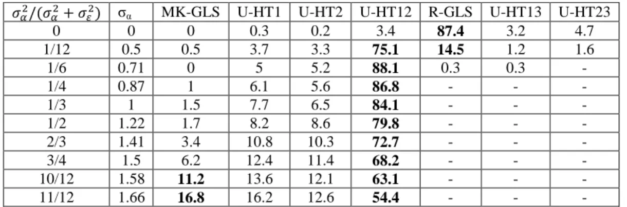
In a …rst set of simulations we changed the variance of the individual e¤ect keeping the overall variance constant. The values of were chosen as in Baltagi et al. (2003, p.368, table 4), namely 2 varying from 0 to 2.75 which corresponds to a variation of 2=( 2 + 2) from 0 to 11/12. Table 1a (all results are reported in appendix B) reports the choice of the pretest estimator for these di¤erent values of . With 2 = 0 the pretest estimator chooses the R-GLS (RE) estimator in 87:4% of all replications and the U-HT12 estimator (unrestricted Hausman Taylor estimator with X1 and X2 as internal instruments, the correct choice given the parametrization of the model) in 3:4% of all replications. With 0:5 2 2:75, the pretest procedure chooses the U-HT12 estimator in at least 54:4% and at most 86:8% replications.
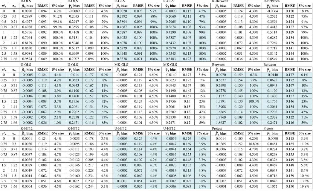
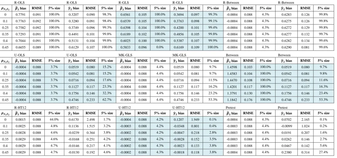
Table 1b reports the bias, the RMSE, and the 5% size for various estimators of 3 and 2. For 2 between 0 and 1, the restricted OLS estimator has the lowest RMSE for 3. Increasing reduces the RMSE for the restricted and unrestricted Hausman Taylor estimator, the within estimator (used at the …rst step of the two-step restricted-between estimator), and the pretest for 3. For 2, R-OLS and R-GLS have the lowest RMSE (0:112), but their value is questionable as they use N T observations in their degrees for freedom. By contrast, between (U-OLS) and restricted and unrestricted Hausman and Taylor estimators have the largest RMSE (0:178), but they use N instead of N T in their degrees of freedom. When increases, the restricted Hausman Taylor RMSE for 2 increases, whereas the between RMSE decreases, as well as the unrestricted Hausman Taylor (U-HT12), because more variance of the dependent variable is explained when including the average-over-time of endogenous time-varying variables.
The R-OLS, between and R-between biases for b3 and b2 are linear increasing functions of , see …gure 1a and …gure 1b. The R-GLS (the usual “random e¤ect" model) bias for b3 increases for value of 2 and then decreases as in Baltagi et al. (2003, p.368). The between estimator has the largest bias for b3 and the smallest bias for b2 of those 3 estimators. The endogeneity bias for b3is fully corrected when including X3i:in the three unrestricted estimators (U-OLS, MK-GLS, U-HT12). The unrestricted OLS and GLS provide the between estimate for the parameter b2. The restricted between is related to a large omitted variable bias for b2. The biases for b3 and for b2 using the restricted Hausman Taylor are negligible. However, they are between 4 to 10 times larger than the one obtained when using the three unrestricted estimators: OLS, GLS and Hausman Taylor. The bias for 2 of the pretest estimator increases …rst because it selects the R-GLS (RE) estimator for = 0:5 in 14:5% of replications, then it falls and increases again when > 1:41, because it increasingly selects the MK-GLS estimator (between estimator for 2), up to 16:8% of replications with = 1:66.
The 5% size columns in tables 1b report the frequency of rejections in 1000 replications of 3 = 1 and 2 = 1, respectively at the 5% signi…cance level. Since the null hypothesis is always true, this represents the empirical size of the test. As expected, R-OLS and R-GLS (RE) estimators perform badly; they reject the (true) null hypothesis frequently, especially when is large. On the other hand, R-HT12 and U-HT12 perform well for 3 and 2, giving the required 5% size, while MK-GLS (FE for 3 and BE for 2) do well for 3 and not so well for 2, with 5% size increasing steadily from around 6% for = 0:5 to 59% for = 1:66. The MK-GLS (BE) for 2 5% sizes are nonetheless smaller than R-OLS, R-GLS and R-BE with 5% size at 100% when > 1. The pretest exceeds the 5% size (reaching 11:2%) for small values of = 0:5 (when it selects the R-GLS (RE) in 14:5% of replications) and then for large values of > 1:41 (reaching 8:5% to 19:8%) because it selects the MK-GLS (BE for 2) in 6.2% to 16.8% of replications.
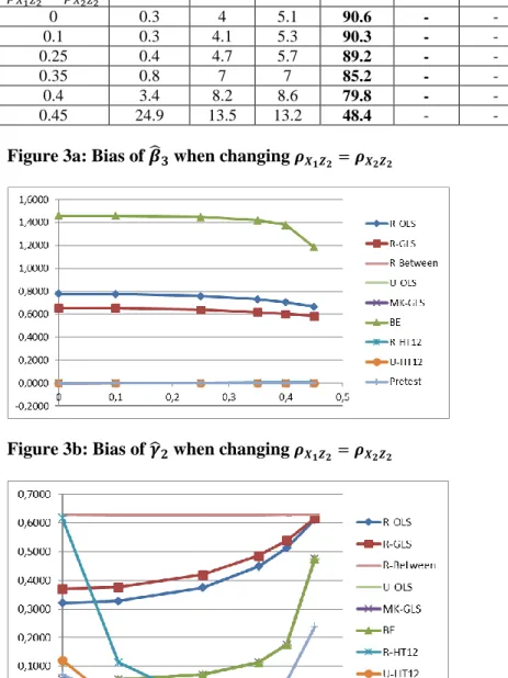
4.2 Changing the degree of endogeneity of the time invariant variable Z2
The correlation between the time-invariant variable and the individual error term indicating the presence of endogeneity has to be contained in the interval 0:426 < Z2 < 0:597 so that
det(R) 0. Table 2a shows that in our simulations the pretest never selected the wrong internal instrument X3. The pretest chooses the correct alternative U-HT12 in 88.6% of all cases for Z2 = 0:5. For large correlations or small correlations also the Mundlak/Krishnakumar
estimator is chosen.
The biases, RMSE and 5% size are presented in table 2b and the biases are shown in …gures 2a and 2b. The restricted OLS estimator, the between estimator and the restricted GLS estimator for 3 are biased and the bias is decreasing when the correlation increases. The other estimators for 3 are performing well with a RMSE and 5% size approximately the same. The bias for 2 increases linearly for R-OLS, R-between, between and non-linearly for R-GLS and the pretest. Restricted and unrestricted Hausman Taylor estimators perform best, even though the unrestricted estimator is slightly better. The less good performance of the pretest comes from the fact that MK-GLS is sometimes chosen. The 5% size of the pretest remains below 19%.
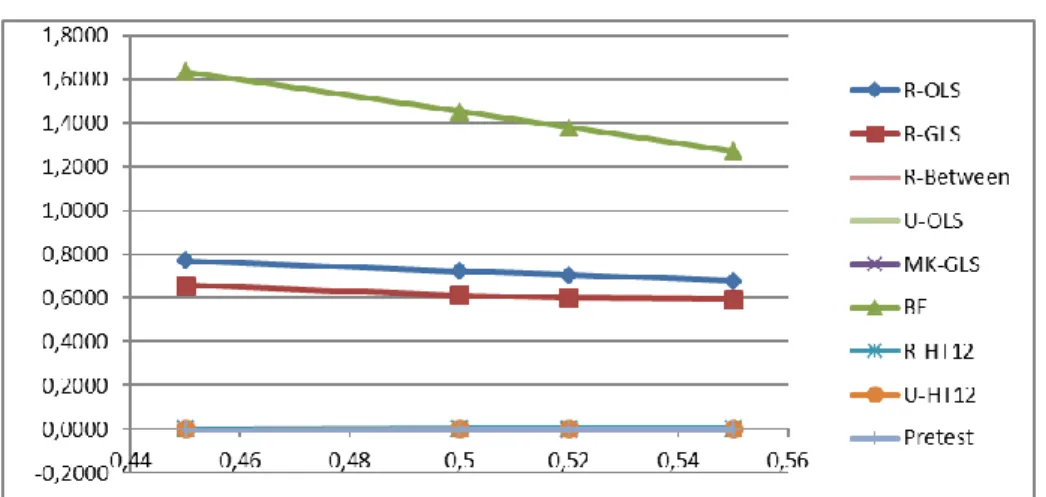
4.3 Shifting from weak to strong internal instruments
Results when increasing simultaneously X1Z2 and X2Z2 ( 0:461 < X1Z2 = X2Z2 < 0:461,
so that det(R) 0)) are presented in tables 3a and 3b. Since the problem is symmetric only the results for positive values, 0 < X1Z2 = X2Z2 < 0:461, are stated.
The percentage of times the pretest selects the di¤erent alternatives when moving from weak to strong internal instruments is shown in table 3a. With the given parametrization the pretest never chooses the wrong instrument. With increasing correlation, however, the pretest chooses also the MK-GLS estimator on takes only one of the averages of the time- and individual varying variables as instrument. This is due to the fact that the overall correlation matrix is nearly non-invertible because of near multi-collinearity. This will be also re‡ected in the biases.
Biases of the estimators, their RMSE and 5% size are shown in table 3b and …gures 3a and 3b. When the internal instruments are weak ( X1Z2 = X2Z2 = 0), the restricted Hausman Taylor
bias is identical to the restricted between bias forb (0:62) which is an intermediate step in the restricted Hausman Taylor estimator. By contrast, the unrestricted Hausman bias forb (0:12) is closer to the bias (0:05) of the between estimator. As a consequence, the pretest estimator has a smaller bias than the restricted Hausman Taylor for weak instruments up to the level: X1Z2 = X2Z2 = 0:25. For large levels of these correlation coe¢ cients ( X1Z2 = X2Z2 = 0:45),
whose square terms also decrease the denominator of the R-OLS bias, the overall correlation matrix R is close to be non invertible because of near-multicollinearity. Then, the bias for 2 tends to increase faster (non linearly) up to the level of the restricted between (0:62) for R-OLS, R-GLS and between, except for the unbiased R-HT12 and U-HT12 estimators which bene…t from strong internal instruments. It is unfortunately also the case for the bias for 1 and 2 in R-OLS, R-GLS and BE, so that the pretest rejects both null hypothesis 1 = 1;BE 1 and 2 = 2;BE 1 and selects the MK-GLS (BE for ) estimator in 24:9% of replications. Its bias is then 0:238 with a 5% size equal to 27% in this limit case.
4.4 Other simulations
To test the robustness of our results, di¤erent levels of signi…cance and di¤erent population size were simulated. Furthermore, the assumptions of normality were relaxed, …rst a uniform distribution for the time-varying error was assumed and secondly a uniform distribution for the individual random disturbance, keeping the overall variance constant.
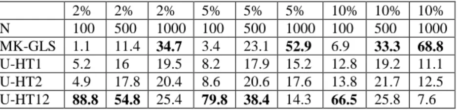
in table 4. The number of individuals went from N = 100 to 500 to 1000. When the sample increases, the absolute value of the t-statistics increases, so that the null hypothesis is more easily rejected, which is also the case when the signi…cance threshold increases from 2% to 5% and to 10%. Then, the pretest selects more often the MK-GLS estimator. In these simulations, the endogenous variable X3 was never selected as exogenous. We can therefore conclude that the pretest performs well for relatively small samples.
When changing the distribution of the disturbances "it from normal to uniform (with iden-tical variance but more kurtosis) the results are almost the same. Details are available from the authors upon request. Chatelain and Ralf (2010) used these various estimators on a wage equation evaluating the returns to schooling on the data set used by Greene (2012), section 11.4.5.
5
Conclusion
When a researcher does not know which are the exogenous internal instruments in order to cor-rect the endogeneity bias of some time-invariant regressors, a pretest estimator based upon the Mundlak-Krishnakumar and an unrestricted Hausman-Taylor estimator is a viable alternative to other estimators in terms of bias, RMSE and inference. The procedures are easy to program since it is only required to compute the average over time of time-varying variables and merge them with the initial data set, and then to use random e¤ects and Hausman-Taylor procedures available e.g. in STATA.
An alternative to Hausman and Taylor (1981) estimator is the FEF-IV estimator for the two-way error component model (Chen, Yue and Wong (2020)) and for the one-two-way error component (Pesaran and Zhou (2018)). Further research may consider pre-tests for instrument selection for these estimators.
Further research may consider the case where the econometricain does not know which time-invariant variables are endogenous. A …nal cross-section instrumental variables (IV) Hausman test upward testing procedure can be tried. In a …rst step, the pre-test Hausman and Taylor (1981) estimator including the best selection of a number of internal instruments at least equal to the number of all time-invariant variables if one …rst assume all of time-invariant variables are endogenous. Hausman and Taylor (1981) provides IV estimates for the set of parameters HT of all time-invariant variables. We have the set of parameters ( + )M K GLS of all time-invariant variables with MK-GLS estimator which may be biased because it assumes that all time-invariant variables are exogenous: = 0. If the null hypothesis of an IV Hausman test H0 : = 0 (if and only if H0 : HT = ( + )M K GLS) is not rejected, then all time-invariant variables are exogenous and MK-GLS is the best linear unbiased estimator. Else, a more precise upward testing procedure (Andrews (1999)) of IV Hausman tests may …nd out if a subset of time-invariant variables are nonetheless exogenous. The remaining subset may have driven the rejection of the null hypothesis when pooling the estimates for all the time-invariant variables in the Hausman (1978) test statistics.
References
[1] Andrews D. (1999). “Consistent Moment Selection Procedures for Generalized Method of Moments Estimation”. Econometrica 67(3). pp.543-564.
[2] Baltagi B. H., Bresson G. and Pirotte A. (2003). Fixed E¤ects, Random E¤ects or Hausman-Taylor? A Pre-test Estimator. Economics Letters. 79, pp. 361-369.
[3] Bouvatier, V. (2014). Heterogeneous bank regulatory standards and the cross-border supply of …nancial services. Economic modelling, 40, 342-354.
[4] Breusch T., Ward M.B., Nguyen H. and Kompas T. (2011). On the …xed e¤ects vector decomposition. Political Analysis, 19, 123-134.
[5] Chatelain, J. B. (2007). Improving consistent moment selection procedures for generalized method of moments estimation. Economics Letters, 95(3), 380-385.
[6] Chatelain, J. B. (2010). Can statistics do without artefacts? Centre Cournot Prisme 19. [7] Chatelain, J. B., and Ralf, K. (2010). Inference on time-invariant variables using panel
data: A pre-test estimator with an application to the returns to schooling. CES working paper.
[8] Chen, J., Yue, R., & Wu, J. (2020). Testing for individual and time e¤ects in the two-way error component model with time-invariant regressors. Economic Modelling, 92, 216-229. [9] Frisch R. and Waugh F.V. (1933). Partial time regression as compared with individual
trends. Econometrica 1, pp. 387-401.
[10] Goh, S. K., & Tham, S. Y. (2013). Trade linkages of inward and outward FDI: Evidence from Malaysia. Economic Modelling, 35, 224-230.
[11] Greene W. (2011). Fixed E¤ects Vector Decomposition: A Magical Solution to the Problem of Time Invariant Variables in Fixed E¤ects Models? Political Analysis, 19, pp. 135-146. [12] Greene W. (2012). Econometric Analysis. 7th edition. Cambridge University Press.
Cam-bridge.
[13] Guggenberger P. (2010). The Impact of a Hausman pretest on the size of a hypothesis test: The Panel data case. Journal of Econometrics 156, pp. 337-343.
[14] Hausman J.A. (1978). Speci…cation Tests in Econometrics. Econometrica 46, pp. 1251-1271. [15] Hausman J.A. and Taylor W.E. (1981). Panel data and unobservable individual e¤ects.
Econometrica 49, pp. 1377-1398.
[16] Hsiao C. (2014). Analysis of Panel Data. 3rd edition. Cambridge University Press. Cam-bridge.
[17] Im K.S., Ahn S.C., Schmidt P. and Wooldridge J.M. (1999). E¢ cient estimation of panel data models with strictly exogenous explanatory variables. Journal of Econometrics 93, pp. 177-203.
[18] Kelejian H.K. and Stephan S.W. (1983). Inference in Random Coe¢ cient Panel Data Mod-els: a Correction and Clari…cation of the Literature. International Economic Review 24, pp. 249-254.
[19] Krishnakumar J. (2006.) Time Invariant Variables and Panel Data Models: A Generalised Frisch-Waugh Theorem and its Implications. in B. Baltagi (editor), Panel Data Economet-rics: Theoretical Contributions and Empirical Applications, published in the series “Con-tributions to Economic Analysis”, North Holland (Elsevier Science), Amsterdam, Chapter 5, 119-132.
[20] Mundlak Y. (1978). On the pooling of time series and cross section data. Econometrica 46, pp. 69-85.
[21] Oaxaca R.L. and Geisler I. (2003). Fixed e¤ects models with time invariant variables: a theoretical note. Economics Letters 80, pp. 373-377.
[22] Pesaran M. H. and Zhou Q. (2018). Estimation of time-invariant e¤ects in static panel data models. Econometric Reviews 37, pp. 1137-1171.
[23] Plümper D. and Troeger V. (2007). E¢ cient Estimation of Time Invariant and Rarely Changing Variables in Finite Sample Panel Analyses with Unit Fixed E¤ects. Political Analysis 15, pp. 124-139.
[24] Serlenga L. and Shin Y. (2007). Gravity models of intra-EU trade: application of the CCEP-HT estimation in heterogeeous panels with unobserved common time-speci…c fac-tors. Journal of Applied Econometrics 22, pp. 361-381.
[25] Swamy P.A.V.B and Arora S.S. (1972). The exact …nite sample properties of the estimators of coe¢ cients in the error components regression models. Econometrica 40, pp. 261-275 [26] Wasserstein, R. L., & Lazar, N. A. (2016). The ASA’s statement on p-values: context,
Appendix A. Unrestricted Hausman and Taylor (U-HT)
estima-tor
If k2 1, to obtain consistent estimators for both and in the second stage, let
b
d = y X bW = B X X0W X
1
X0W y
be the N T vector of group means estimated from the within-groups residuals. The only di¤er-ence of the unrestricted Hausman and Taylor with respect to the usual restricted Hausman and Taylor is to keep the average over time of the endogenous time varying variables X2 in each of the steps derived by Hausman and Taylor (1981). Expanding this expression using equation 4 including only X2leads to:
b
d = Z1 1+ Z2( 2+ 2) + X2 3+ M + B X X0W X
1
X0W ": (11)
Treating the last two terms as an unobservable mean zero disturbance, we estimate from the above equation using N observations. If is correlated with the columns of Z2, E ( j Z2) = 26= 0, according to prior information, both OLS and GLS will be inconsistent estimators for . Consistent estimation is possible, however, if the columns of X1, uncorrelated with according to the non rejection of the null hypothesis of preliminary tests, provide su¢ cient instruments for the columns of Z in equation (11). The two stage least squares (2SLS) estimator for in equation (11) is:
bII = Z0; X2 PA Z0; X2 1
Z0; X2 0PAdb (12)
where A = X1; Z1 and PAis the orthogonal projection operator onto its column space. The sampling error is given by
bII = Z0; X2 PA Z0; X2 1
Z0; X2 0PA M + B X X0W X
1
X0W "
and under the usual assumptions governing X and Z, the 2SLS estimator is consistent for , since for …xed T , plimN !1N1A0 = 0 and plimN !1N1X0" = 0.
Having consistent estimators of and, under the condition k1 g2, , we can construct consistent estimators for the variance components. A consistent estimator of 2" can be derived from the within-group residuals in the …rst step c2
" = M SEW. Whenever we have consistent
estimators for both and , a consistent estimator for 2 can be obtained. Let
s2 = (1=N ) y X bW ZbII X2b2;II 0 y X bW ZbII X2b2;II then plim N !1 s2= plim N !1 1 N ( + ") 0( + ") = 2 + 1 T 2 " so that s2a= s2 (1=T ) s2" is consistent for s2a.
Appendix B
Table 1a: Percentage of times the pretest selects the internal instruments when changing σα 𝜎𝛼2/(𝜎𝛼2+ 𝜎𝜀2) σα MK-GLS U-HT1 U-HT2 U-HT12 R-GLS U-HT13 U-HT23
0 0 0 0.3 0.2 3.4 87.4 3.2 4.7 1/12 0.5 0.5 3.7 3.3 75.1 14.5 1.2 1.6 1/6 0.71 0 5 5.2 88.1 0.3 0.3 - 1/4 0.87 1 6.1 5.6 86.8 - - - 1/3 1 1.5 7.7 6.5 84.1 - - - 1/2 1.22 1.7 8.2 8.6 79.8 - - - 2/3 1.41 3.4 10.8 10.3 72.7 - - - 3/4 1.5 6.2 12.4 11.4 68.2 - - - 10/12 1.58 11.2 13.6 12.1 63.1 - - - 11/12 1.66 16.8 16.2 12.6 54.4 - - -
Figure 1a: Bias of 𝜷̂𝟑 when changing σα
Table 1b: Bias. RMSE and 5% size test for 𝜷̂𝟑 and 𝜸̂𝟐 in a Hausman-Taylor world, 1000 replications, N=100 and T=5, changing the variance of the individual effect
R-OLS R-OLS R-GLS R-GLS R-Between R-Between
σ²α σα 𝜷̂𝟑 bias RMSE 5% size 𝜸̂𝟐 bias RMSE 5% size 𝜷̂𝟑 bias RMSE 5% size 𝜸̂𝟐 bias RMSE 5% size 𝜷̂𝟑 bias RMSE 5% size 𝜸̂𝟐 bias RMSE 5% size
0 0 0.0020 0.094 6.2% -0.0089 0.112 4.8% 0.0020 0.093 5.7% -0.0090 0.112 4.2% -0.0005 0.124 4.30% -0.0064 0.120 18.1% 0.25 0.5 0.2889 0.093 91.2% 0.2035 0.111 49% 0.2792 0.094 88% 0.2060 0.111 47% -0.0005 0.119 4.30% 0.2522 0.122 75% 0.5 0.71 0.4077 0.093 99.1% 0.2917 0.109 79% 0.3894 0.094 99% 0.2965 0.110 79% -0.0005 0.113 4.30% 0.3594 0.124 91% 0.75 0.87 0.4988 0.092 99.9% 0.3595 0.108 93% 0.4687 0.095 100% 0.3674 0.108 93% -0.0005 0.108 4.30% 0.4418 0.127 97% 1 1 0.5756 0.092 100.0% 0.4168 0.107 99% 0.5287 0.097 100% 0.4290 0.108 99% -0.0004 0.101 4.30% 0.5114 0.129 99% 1.5 1.22 0.7044 0.091 100.0% 0.5131 0.104 100% 0.6025 0.100 100% 0.5387 0.107 100% -0.0004 0.088 4.30% 0.6282 0.134 100% 2 1.41 0.8129 0.090 100.0% 0.5946 0.101 100% 0.6078 0.100 100% 0.6432 0.107 100% -0.0003 0.072 4.30% 0.7269 0.139 100% 2.25 1.5 0.8620 0.089 100.0% 0.6317 0.099 100% 0.5729 0.098 100% 0.6970 0.109 100% -0.0003 0.062 4.30% 0.7717 0.141 100% 2.5 1.58 0.9084 0.089 100.0% 0.6669 0.098 100% 0.4948 0.091 100% 0.7543 0.113 100% -0.0002 0.051 4.30% 0.8142 0.144 100% 2.75 1.66 0.9524 0.089 100.0% 0.7007 0.096 100% 0.3378 0.071 100% 0.8183 0.123 100% -0.0002 0.036 4.30% 0.8549 0.146 100%
U-OLS U-OLS MK-GLS MK-GLS Between Between
σ²α σα 𝜷̂𝟑 bias RMSE 5% size 𝜸̂𝟐 bias RMSE 5% size 𝜷̂𝟑 bias RMSE 5% size 𝜸̂𝟐 bias RMSE 5% size 𝜷̂𝟑 bias RMSE 5% size 𝜸̂𝟐 bias RMSE 5% size
0 0 -0.0005 0.124 4.4% -0.014 0.177 5.9% -0.0005 0.124 4.60% -0.0140 0.177 5.5% 0.0070 0.159 6.3% -0.0140 0.177 6.1% 0.25 0.5 -0.0005 0.119 4.2% 0.0623 0.172 8% -0.0005 0.119 4.60% 0.0623 0.172 7% 0.5677 0.154 97% 0.0623 0.172 8% 0.5 0.71 -0.0005 0.113 4.1% 0.0943 0.167 11% -0.0005 0.113 4.60% 0.0943 0.167 10% 0.7998 0.150 100% 0.0943 0.167 10% 0.75 0.87 -0.0005 0.108 3.9% 0.1190 0.162 14% -0.0005 0.108 4.60% 0.1190 0.162 12% 0.9778 0.145 100% 0.1190 0.162 12% 1 1 -0.0004 0.101 3.8% 0.1400 0.157 18% -0.0004 0.101 4.50% 0.1400 0.157 15% 1.1277 0.140 100% 0.1400 0.157 15% 1.5 1.22 -0.0004 0.088 3.7% 0.1756 0.146 32% -0.0005 0.124 4.60% 0.1756 0.15 23% 1.3791 0.130 100.0% 0.1756 0.146 23% 2 1.41 -0.0003 0.072 3.3% 0.2061 0.134 51% -0.0005 0.119 4.60% 0.2061 0.13 35% 1.5908 0.120 100% 0.2061 0.134 35% 2.25 1.5 -0.0003 0.062 2.9% 0.2202 0.128 62% -0.0005 0.113 4.60% 0.2202 0.13 42% 1.6865 0.114 100% 0.2202 0.128 42% 2.5 1.58 -0.0002 0.051 2.1% 0.2338 0.122 73% -0.0005 0.108 4.60% 0.2338 0.12 51% 1.7769 0.108 100% 0.2338 0.122 51% 2.75 1.66 -0.0002 0.036 1.0% 0.2471 0.116 85% -0.0004 0.101 4.50% 0.2471 0.12 59% 1.8627 0.102 100% 0.2471 0.116 59%
R-HT12 R-HT12 U-HT12 U-HT12 Pretest Pretest
σ²α σα 𝜷̂𝟑 bias RMSE 5% size 𝜸̂𝟐 bias RMSE 5% size 𝜷̂𝟑 bias RMSE 5% size 𝜸̂𝟐 bias RMSE 5% size 𝜷̂𝟑 bias RMSE 5% size 𝜸̂𝟐 bias RMSE 5% size
0 0 0.0001 0.124 4.4% -0.0053 0.178 3.5% -0.0003 0.124 4.4% -0.0056 0.176 4.0% 0.0014 0.100 6.20% -0.0090 0.118 3.9% 0.25 0.5 0.0030 0.119 4.7% -0.0095 0.186 4.5% -0.0003 0.119 4.4% -0.0047 0.169 3.9% 0.0265 0.152 16.80% 0.0461 0.185 11.2% 0.5 0.71 0.0036 0.114 4.7% -0.0111 0.193 4.4% -0.0003 0.114 4.4% -0.0041 0.164 3.6% 0.0006 0.115 4.70% 0.0224 0.164 3.2% 0.75 0.87 0.0037 0.108 4.7% -0.0123 0.199 4.6% -0.0003 0.108 4.4% -0.0036 0.155 3.8% -0.0002 0.108 4.50% 0.0268 0.155 3.3% 1 1 0.0035 0.102 4.6% -0.0132 0.205 4.4% -0.0003 0.102 4.2% -0.0032 0.148 3.7% -0.0003 0.102 4.30% 0.0326 0.149 3.8% 1.5 1.22 0.0029 0.088 4.7% -0.0146 0.217 4.1% -0.0003 0.088 4.3% -0.0023 0.133 3.8% -0.0003 0.088 4.40% 0.0467 0.148 5.6% 2 1.41 0.0019 0.072 4.7% -0.0156 0.228 4.2% -0.0002 0.072 4.4% -0.0013 0.115 3.8% -0.0003 0.072 4.50% 0.0633 0.141 8.5% 2.25 1.5 0.0014 0.062 4.5% -0.0160 0.234 4.3% -0.0002 0.062 4.4% -0.0008 0.106 3.9% -0.0002 0.062 4.50% 0.0716 0.139 10.6% 2.5 1.58 0.0009 0.051 4.6% 0.0162 0.239 4.8% 0.0001 0.051 4.4% 0.0002 0.095 3.8% 0.0002 0.051 4.50% 0.0846 0.143 13.8% 2.75 1.66 0.0004 0.036 4.5% -0.0162 0.244 5.1% -0.0001 0.036 4.3% 0.0006 0.083 3.7% -0.0001 0.036 4.30% 0.1052 0.150 19.8%
Table 2a: Percentage of times the pretest selects the internal instruments when changing 𝝆𝒁 𝟐𝜶
𝜌𝑍2𝛼 MK-GLS U-HT1 U-HT2 U-HT12 R-GLS U-HT13 U-HT23
0.45 4.2 10.7 11.4 73.74 - - -
0.5 0.7 5.7 5 88.6 - - -
0.52 3.4 8.2 8.6 79.8
0.55 14.2 14.2 16.2 51.1 - - -
Figure 2a: Bias of 𝜷̂𝟑 when changing 𝝆𝒁𝟐𝜶