HAL Id: hal-00979044
https://hal.inria.fr/hal-00979044
Submitted on 15 Apr 2014HAL is a multi-disciplinary open access archive for the deposit and dissemination of sci-entific research documents, whether they are pub-lished or not. The documents may come from
L’archive ouverte pluridisciplinaire HAL, est destinée au dépôt et à la diffusion de documents scientifiques de niveau recherche, publiés ou non, émanant des établissements d’enseignement et de
A New Walk on Equations Monte Carlo Method for
Linear Algebraic Problems
Ivan Tomov Dimov, Sylvain Maire, Jean-Michel Sellier
To cite this version:
Ivan Tomov Dimov, Sylvain Maire, Jean-Michel Sellier. A New Walk on Equations Monte Carlo Method for Linear Algebraic Problems. Applied Mathematical Modelling, Elsevier, 2015, 39 (15), �10.1016/j.apm.2014.12.018�. �hal-00979044�
A New Walk on Equations Monte Carlo
Method for Linear Algebraic Problems ⋆
Ivan Dimov
a,∗ Sylvain Maire
bJean Michel Sellier
caDepartment of Parallel Algorithms, IICT, Bulgarian Academy of Sciences, Acad.
G. Bonchev 25 A, 1113 Sofia, Bulgaria
bLaboratoire LSIS Equipe Signal et Image, Universit´e du Sud Toulon-Var, AV.
Georges Pompidou BP 56 83162 La Valette du Var Cedex
cDepartment of Parallel Algorithms, IICT, Bulgarian Academy of Sciences, Acad.
G. Bonchev 25 A, 1113 Sofia, Bulgaria
Abstract
A new Walk on Equations (WE) Monte Carlo algorithm for Linear Algebra (LA) problem is proposed and studied. This algorithm relies on a non-discounted sum of an absorbed random walk. It can be applied for either real or complex matrices. Several techniques like simultaneous scoring or the sequential Monte Carlo method are applied to improve the basic algorithm. Numerical tests are performed on exam-ples with matrices of different size and on systems coming from various applications. Comparisons with standard deterministic or Monte Carlo algorithms are also done.
Key words: Monte Carlo algorithms, Markov chain, eigenvalue problem, robust algorithms.
1991 MSC: 65C05, 65U05, 65F10, 65Y20
⋆ This work was partially supported by the European Commission under FP7 project AComIn (FP7 REGPOT-2012-2013-1, by the Bulgarian NSF Grant DCVP 02/1, as well as by the Universit´e du Sud Toulon-Var.
∗ Corresponding author.
Email addresses: [email protected] (Ivan Dimov), [email protected] (Sylvain Maire), [email protected] (Jean Michel Sellier).
URLs: http://parallel.bas.bg/dpa/BG/dimov/index.html (Ivan Dimov), http://maire.univ-tln.fr/(Sylvain Maire), http://www.bas.bg (Jean Michel Sellier).
1 Introduction
In this paper we analyze applicability and efficiency of the proposed WE algo-rithm. The algorithm is based on Markov chain Monte Carlo (MC) approach. We focus our consideration to real symmetric matrices, but a wider class of matrices can also be treated.
Many scientific and engineering applications are based on the problems of solving systems of linear algebraic equations. For some applications it is also important to compute directly the inner product of a given vector and the solution vector of a linear algebraic system. For many LA problems it is im-portant to be able to find a preconditioner with relatively small computational complexity. That is why, it is important to have relatively cheap algorithm for matrix inversion. The computation time for very large problems, or for finding solutions in real-time, can be prohibitive and this prevents the use of many established algorithms. Monte Carlo algorithms give statistical estimates of the required solution, by performing random sampling of a random variable, whose mathematical expectation is the desired solution [2,3,7,23,29–31]. Let J be the exact solution of the problem under consideration. Suppose it is proved that there exists a random variable θ, such that E{θ} = J. If one can produce N values of θ, i.e. θ1, . . . , θN, then the value ¯θN = ∑Ni=1θN can
be considered as a Monte Carlo (MC) approximation of J. The probability error of the MC algorithm is defined as the least possible real number RN, for
which: P = P r{|∑Ni=1θN − J| ≤ RN}, where 0 < P < 1.
Several authors have presented works on MC algorithms for LA problems and on the estimation of computational complexity [1,6,15,8,10,11]. There are MC algorithms for
• computing components of the solution vector; • evaluating linear functionals of the solution; • matrix inversion, and
• computing the extremal eigenvalues.
An overview of all these algorithms is given in [7]. The well-known Power method [17] gives an estimate for the dominant eigenvalue λ1. This estimate
uses the so-called Rayleigh quotient. In [9] the authors consider bilinear forms of matrix powers, which is used to formulate a solution for the eigenvalue problem. A Monte Carlo approach for computing extremal eigenvalues of real symmetric matrices as a special case of Markov chain stochastic method for computing bilinear forms of matrix polynomials is considered. In [9] the ro-bustness and applicability of the Almost Optimal Monte Carlo algorithm for solving a class of linear algebra problems based on bilinear form of matrix powers (v, Ak). It is shown how one has to choose the acceleration parameter
q in case of using Resolvent Power MC. The systematic error is analyzed and it is shown that the convergence can not be better than O( 1+|q|λn
1+|q|λn−1
)m
, where λn is the smallest by modulo eigenvalue, q is the characteristic parameter,
and m is the number of MC iterations by the resolvent matrix. To construct an algorithm for evaluating the minimal by modulo eigenvalue λn, one has to
consider the following matrix polynomial pk(A) = ∑∞k=0qkCm+k−1k Ak, where
Ck
m+k−1 are binomial coefficients, and the characteristic parameter q is used
as acceleration parameter of the algorithm [8,12,13]. This approach is a dis-crete analogues of the resolvent analytical continuation method used in the functional analysis [24]. There are cases when the polynomial becomes the resolvent matrix [11,12,7]. It should be mentioned that the use of acceleration parameter based on the resolvent presentation is one way to decrease the com-putational complexity. Another way is to apply a variance reduction technique [4] in order to get the required approximation of the solution with a smaller number of operations. The variance reduction technique for particle trans-port eigenvalue calculations proposed in [4] uses Monte Carlo estimates of the forward and adjoint fluxes. In [27] an unbiased estimation of the solution of the system of linear algebraic equations is presented. The proposed estimator can be used to find one component of the solution. Some results concerning the quality and the properties of this estimator are presented. Using this es-timator the author gives error bounds and constructs confidence intervals for the components of the solution. In [16] a Monte Carlo algorithm for matrix inversion is proposed and studied. The algorithm is based on the solution of simultaneous linear equations. In our further consideration we will use some results from [16] and [7] to show how the proposed algorithm can be used for approximation of the inverse of a matrix.
2 Formulation of the Problem: Solving Linear Systems and Matrix Inversion
By A and B we denote matrices of size n × n, i.e., A, B ∈ IRn×n. We use the
following presentation of matrices:
A = {aij}ni,j=1 = (a1, . . . , ai, . . . , an)t,
where ai = (ai1, . . . , ain), i = 1, . . . , n and the symbol t means transposition.
The following norms of vectors (l1-norm):
∥ b ∥=∥ b ∥1= n ∑ i=1 |bi|, ∥ ai ∥=∥ ai ∥1= n ∑ j=1 |aij|
and matrices ∥ A ∥=∥ A ∥1= max j n ∑ i=1 |aij| are used.
Consider a matrix A ∈ IRn×n and a vector b = (b1, . . . , bn)t ∈ IRn×1. The
matrix A can be considered as a linear operator A[IRn → IRn] [24,7], so that
the linear transformation
Ab ∈ IRn×1 (1)
defines a new vector in IRn×1.
Since iterative Monte Carlo algorithms using the transformation (1) will be considered, the linear transformation (1) is called iteration. The algebraic transformation (1) plays a fundamental role in the iterative Monte Carlo al-gorithms [7].
Now consider the following three LA problems Pi (i=1,2,3): Problem P1. Evaluating the inner product
J(u) = (v, x) =
n
∑
i=1
vixi
of the solution x ∈ IRn×1 of the linear algebraic system
Bx = f,
where B = {bij}ni,j=1 ∈ IRn×n is a given matrix; f = (f1, . . . , fn)t ∈ IRn×1 and
v = (v1, . . . , vn)t∈ IRn×1 are given vectors.
It is possible to choose a non-singular matrix M ∈ IRn×n such that M B =
I − A, where I ∈ IRn×n is the identity matrix and M f = b, b ∈ IRn×1.
Then
x = Ax + b. (2)
It will be assumed that
(i)
1. The matrices M and A are both non-singular; 2. |λ(A)| < 1 for all eigenvalues λ(A) of A,
that is, all values λ(A) for which
Ax = λ(A)x
is satisfied. If the conditions (i) are fulfilled, then a stationary linear iterative
algorithm [7,6] can be used:
xk = Axk−1+ b, k = 1, 2, . . . (3)
and the solution x can be presented in a form of a von Neumann series x =
∞
∑
k=0
Akb = b + Ab + A2b + A3b + . . . (4)
The stationary linear iterative Monte Carlo algorithm [7,6] is based on the above presentation and will be given later on. As a result, the convergence of the Monte Carlo algorithm depends on the truncation error of the series (3) (see, [7]).
Problem P2. Evaluating all components xi, i = 1, . . . n of the solution
vec-tor.
In this case we deal with the equation (2) assuming that A = I − M B, as well as, b = M f .
Problem P3. Inverting of matrices, i.e. evaluating of matrix G = B−1,
where B ∈ IRn×n is a given real matrix.
Assumed that the following conditions are fulfilled:
(ii)
1. The matrix B is non-singular;
2. ||λ(B)| − 1| < 1 for all eigenvalues λ(B) of B.
Obviously, if the condition (i) is fulfilled, the solution of the problem P1 can be obtained using the iterations (3).
For problem P3 the following iterative matrix: A = I − B can be constructed.
Since it is assumed that the conditions (ii) are fulfilled, the inverse matrix G = B−1 can be presented as G = ∞ ∑ i=0 Ai.
For problems Pi(i = 1, 2, 3) one can create a stochastic process using the
matrix A and vectors b, and possibly v.
Consider an initial density vector p = {pi}ni=1 ∈ IRn, such that pi ≥ 0, i =
1, . . . , n and ∑n
i=1pi = 1. Consider also a transition density matrix P =
{pij}ni,j=1 ∈ IRn×n, such that pij ≥ 0, i, j = 1, . . . , n and ∑nj=1pij = 1, for
any i = 1, . . . , n. Define sets of permissible densities Pb and PA.
Definition 2.1 The initial density vector p = {pi}ni=1 is called permissible
to the vector b = {bi}ni=1 ∈ IRn , i.e. p ∈ Pb, if
pαs > 0 when vαs ̸= 0 pαs = 0 when vαs = 0. (5)
Similarly, the transition density matrix P = {pij}ni,j=1 is called permissible to
the matrix A = {aij}ni,j=1, i.e. P ∈ PA, if
pαs−1,αs > 0 when aαs−1,αs ̸= 0 pαs−1,αs = 0 when aαs−1,αs = 0. (6)
In this work we will be dealing with with permissible densities. It is obvious that in such a way the random trajectories constructed to solve the problems under consideration never visit z ero elements of the matrix. Such an approach decreases the computational complexity of the algorithms. It is also very con-venient when large sparse matrices are to be treated.
We shall use the so-called MAO algorithm studied in [7,6,5,9]. Here we give a brief presentation of MAO. Suppose we have a Markov chain:
T = α0 → α1 → . . . αk → . . . , (7)
with n states. The random trajectory (chain) Tk of length k starting in the
state α0 is defined as follows:
where αj means the number of the state chosen, for j = 1, . . . , n.
Assume that
P (α0 = α) = pα and P (αj = β|αj−1 = α) = pαβ, (9)
where pα is the probability that the chain starts in state α and pαβ is the
tran-sition probability to state β after being in state α. Probabilities pαβ define a
transition matrix P . For the standard Markov chain Monte Carlo we normally require that n ∑ α=1 pα = 1 and n ∑ β=1 pαβ = 1 for any α = 1, . . . , n. (10)
The above allows the construction of the following random variable, that is a unbiased estimator for the Problem P1:
θ[b] = bα0 p0 ∞ ∑ m=0 Qmbαm , (11) where Q0 = 1; Qm = Qm−1 aαm−1,αm pαm−1,αm , m = 1, 2, . . . (12)
and α0, α1, . . . is a Markov chain on elements of the matrix A constructed
by using an initial probability p0 and a transition probability pαm−1,αm for choosing the element aαm−1,αm of the matrix A.
Now define the random variables Qm using the formula (12). One can see, that
the random variables Qm, m = 1, . . . , i can also be considered as weights on
the Markov chain (7).
One possible possible permissible densities can be chosen in the following way: p = {pα}nα=1 ∈ Pb, pα = |bα| ∥ b ∥; P = {pαβ}nα,β=1 ∈ PA, pαβ = |aαβ| ∥ aα ∥ , α = 1, . . . , n. (13)
Such a choice of the initial density vector and the transition density matrix leads to an Almost Optimal Monte Carlo (MAO) algorithm (see [5,7]). The initial density vector p = {pα}nα=1 is called almost optimal initial density vector
and the transition density matrix P = {pαβ}nα,β=1 is called almost optimal
density matrix [5].
Let us consider Monte Carlo algorithms with absorbing states: instead of the finite random trajectory Tiin our algorithms we consider an infinite trajectory
with a state coordinate δi(i = 1, 2, . . .). Assume δi = 0 if the trajectory is
broken (absorbed) and δi = 1 in other cases. Let
∆i = δ0× δ1× . . . × δi.
So, ∆i = 1 up to the first break of the trajectory and ∆q= 0 after that.
It is easy to show, that under the conditions (i) and (ii), the following equalities are fulfilled: E{Qifki} = (h, A ib), i = 1, 2, . . . ; E{ N ∑ i=0 ∆iQibki} = (h, x), (P 1), E{ ∑ i|ki=r′ ∆iQi} = crr′, (P 3),
where (i|ki = r′) means a summation only for weights Qi for which ki = r′
and C = {crr′}nr,r′=1.
The new WE algorithm studied in this paper was proposed by the second author. One important difference from the previously known Markov chain Monte Carlo algorithms is the special choice of the absorbtion probabilities. In this case the Markov chain has n+1 states, {1, . . . , n, n+1}. The transition density matrix (10) is such that∑nβ=1pαβ ≤ 1 and the probability for
absorb-tion at each stage accept the starting one is pα,n+1 = pα = 1 −∑nβ=1pαβ, α =
1, . . . , n.
3 Description of the probabilistic representation for the WE algo-rithm
We start the description of the probabilistic representation of the algorithm with two simple examples. The first example is for the case when all the coefficients of the matrix are non-negative. The second example deals with the case when some matrix coefficients may be negative real numbers. In this section we give a probabilistic representation for the WE algorithm for real-valued matrices, as well as for complex-real-valued ones.
3.1 A simple example: the positive case
We start with a simple example of positive case meaning that aij ≥ 0, i, j =
1, . . . , n. For simplicity, we also assume that ∑nj=1aij ≤ 1.
We describe on a very simple example how we obtain our probabilistic repre-sentation. We consider the system of two equations:
x1 = 1 2x1+ 1 4x2+ 1, x2 = 1 3x1+ 1 3x2+ 2
with unknowns x1 and x2. We have obviously x1 = 1 + E(X) where
P (X = x1) = 1 2, P (X = x2) = 1 4, P (X = 0) = 1 4 and x2 = 2 + E(Y ) where
P (Y = x1) = 1 3, P (Y = x2) = 1 3, P (Y = 0) = 1 3.
We will use only one sample to approximate the expectations and compute a score initialized by zero along a random walk on the two equations. For instance, to approximate x1 we add 1 to the score of our walk and then either
we stop with probability 14 because we know the value of X which is zero or either we need again to approximate x(1) or u(2) with probability 1
2 or
1
4. If the walk continues and that we need to approximate x(2), we add 2 to
the score of our walk, we stop with probability 13 or either we need again to approximate x1 or x(2) with probability 13. The walk continues until one of the
random variables X or Y takes the value zero and the score is incremented along the walk as previously. The score is an unbiased estimator of x1 and
we make the average of the scores of independent walks to obtain the Monte Carlo approximation of x1.
This algorithm is very similar to the ones used to compute the Feynman-Kac representations of boundary value problems by means of discrete or continuous walks like walk on discrete grids or the walk on spheres method. At each step of the walk, the solution at the current position x is equal to the expectation of the solution on a discrete or continuous set plus eventually a source term. The key ingredient is the double randomization principle which says that we can replace the expectation of the solution on this set by the solution at one random point picked according to the appropriate distribution. For example, for the walk on spheres methods this distribution is the uniform law on the sphere centered at x and of radius the distance to the boundary.
3.2 Simple example: general real matrix
We slightly modify our system by considering now the system of two equations x1 = 1 2x1− 1 4x2+ 1, x2 = 1 3x1+ 1 3x2+ 2
with unknowns x1 and x2. We have x1 = 1 + E(W ) where
P (W = x1) = 1 2, P (W = −x2) = 1 4, P (W = 0) = 1 4 and x2 = 2 + E(Z) where
P (Z = x1) = 1 3, P (Z = x2) = 1 3, P (Z = 0) = 1 3.
To approximate x1 we add 1 to the score of our walk and then either we stop
with probability 1
4 because we know the value of X which is zero or either we
need to approximate x1 or −x2 with probability 12 or 14. If the walk continues
and that we need to approximate −x2, we add −2 to the score of our walk,
we stop with probability 1
3 or either we need to approximate −x1 or −x2 with
probability 13. If the walk continues again and that we need to approximate −x1, we add −1 to the score of our walk, we stop with probability 14 or either
we need to approximate −x1 or x2 with probability 12 or 14. The walk continues
until one of the random variables W or Z takes the value zero and the score is incremented along the walk as previously. The same kind of reasoning holds for a complex-valued matrix in the representation given later on in Subsection 3.4.
3.3 Probabilistic representation for real matrices
Consider a real linear system of the form u = Au + b where the matrix A of size n is such that ϱ(A) < 1, its coefficients ai,j are real numbers and
n
∑
j=1
|ai,j| ≤ 1, ∀1 ≤ i ≤ n.
We now define a Markov chain Tkwith n + 1 states α1, . . . , αn, n + 1, such that
if i ̸= n + 1 and
P (αk+1 = n + 1/αk = n + 1) = 1.
We also define a vector c such that c(i) = b(i) if 1 ≤ i ≤ n and c(n + 1) = 0. Denote by τ = (α0, α1, . . . , αk, n + 1) a random trajectory that starts at the
initial state α0 < n + 1 and passes through (α1, . . . , αk) until the absorbing
state αk+1 = n + 1. The probability to follow the trajectory τ is P (τ ) =
pα0pα0α1, . . . pαk−1,kαkpαk. We use the MAO algorithm defined by (13) for the initial density vector p = {pα}nα=1 and for the transition density matrix P =
{pαβ}nα,β=1, as well. The weights Qα are defined in the same way as in (12),
i.e., Qm = Qm−1 aαm−1,αm pαm−1,αm , m = 1, . . . , k, Q0 = cα0 pα0 . (14)
The estimator θα(τ ) can be presented as θα(τ ) = cα+ Qk aαkα
pαk , α = 1, . . . n
taken with a probability P (τ ) = pα0pα0α1, . . . pαk−1,kαkpαk.
Now, we can prove the following theorem.
Theorem 3.1 The random variable θα(τ ) is an unbiased estimator of xα, i.e.
E{θα(τ )} = xα. P r o o f. E{θα(τ )}= ∑ τ=(α0,...,αk,n+1) θα(τ )P (τ ) = ∑ τ=(α0,...,αk,n+1) ( cα+ Qk(τ ) aαkα pαk ) P (τ ) = cα+ ∑ τ=(α0,...,αk,n+1) Qk(τ ) aαkα pαk P (τ ) = cα+ ∑ τ=(α0,...,αk,n+1) cα0 pα0 aα0α1. . . aαk−1αk pα0α1. . . pαk−1αk aαkα pαk pα0 × pα0α1. . . pαk−1αkpαk = cα+ ∞ ∑ k=0 n ∑ α0=1 . . . n ∑ αk=1 aαkαaαk−1αk. . . aα0α1cα0 = cα+ (Ac)α+ (A2c)α+ . . .
= (∞ ∑ i=0 ( Aic) ) α . (15)
Since ϱ(A) < 1, the last sum in (15) is finite and
(∞ ∑ i=0 ( Aic) ) α = xα, α = 1, . . . , n. Thus, E{θα(τ )} = xα. ♢
Let as stress on the fact that among elements cα0, aα0α1. . . aαk−1αk there are no elements equal to zero because of the special choice of permissible distributions pα and pαβ defined by MAO densities (13). The rules (13) ensure that the
Markov chain visits non-zero elements only.
One may also observe that the conjugate to θα(τ ) random variable θ∗α(τ ) =
∑k
i=0Qi
aαiα
pαi cαhas the same mean value, i.e., xα. It can be immediately checked
following the same technique as in the proof of Theorem 3.1.
Assume one can compute N values of the random variable θα, namely θα,i, i =
1, . . . , N . Let us consider the value ¯θα,N = N1 ∑Ni=1θα,i as a Monte Carlo
ap-proximation of the component xα of the solution. For the random variable
¯
θα,N the following theorem is valid:
Theorem 3.2 The random variable ¯θα,N is an unbiased estimator of xα, i.e.
E{¯θα,N} = xα (16)
and the variance D{¯θα,N} vanishes when N goes to infinity, i.e
lim
N→∞D{¯θα,N} = 0. (17)
P r o o f. Equality (16) can easily be proved using properties of the mean value. Using the variance properties one can also show that (17) is true. ♢ Moreover, using the Kolmogorov theorem and the fact that the sequences (θα,N)N≥1 are independent and also independently distributed with a finite
mathematical expectation equal to xαone can show that ¯θα,N converges almost
surely to xα:
P ( lim
N→∞
¯
The theorems proved (Th.3.1 and Th.3.2) with the last fact allows us to use the Monte Carlo method with the random variable θα for solving algebraic
systems and ensure that the estimate is unbias and converges almost surely to the solution. These facts do not give us a measure of the rate of convergence and do not answer the question how one could control the quality of the Monte
Carlo algorithm? At the same time it is clear that the quality of the algorithm,
meaning how fast is the convergence and how small is the probability error, should depend on the properties of the matrix A, and possibly of the right-hand side vector b. Our study shows that the balancing of the matrix together with the matrix spectral radius is an important issue for the quality of the Monte Carlo algorithm. And this is important for all three problems under consideration. To analyse this issue let us consider the variance of the random variable θα(τ ) for solving Problem P1, i.e., evaluating the inner product
J(x) = (v, x) =
n
∑
i=1
vixi
of a given vector v = (v1, . . . , vn)t ∈ IRn×1 and the solution x of the system
(2):
x = Ax + b, A ∈ IRn×n, b = (b1, . . . , bn)t∈ IRn×1.
By chousing v to be an unit vector e(j)≡ (0, . . . , 0, 1
|{z}
j
, 0, . . . , 0) all elements, of which are zeros except the jthelement e(j)
j , which is equal to 1 the functional
J(x) becomes equal to xj. Denote by ¯A the matrix containing the absolute
values of elements of a given matrix A: ¯A = {|aij|}ni,j=1 and by ˆc the vector of
squared entrances of the vector c, i.e., ˆc = {c2
i}n+1i=1. The pair of MAO density
distributions (13) define a finite chain of vector and matrix entrances:
cα0 → aα0α1 → . . . → aαk−1αk. (18)
The latter chain induces the following product of matrix/vector entrances and norms: Ak c = cα0 k ∏ s=1 aαs−1αs,
where the vector c ∈ IRn×1 is defined as c(i) = b(i) if 1 ≤ i ≤ n and c(n + 1) =
0. Obviously, the variance of the random variable ψk
α(τ ) defined as ψαk(τ ) = cα0 pα0 aα0α1 pα0α1 aα1α2 pα1α2 . . .aαk−1αk pαk−1αk cαk pαk = A k ccαk Pk(τ )
plays an important role in defining the quality of the proposed WE Monte Carlo algorithm. Smaller is the variance of D{ψk
α(τ )}, better convergency of
the algorithm will be achieved.
Theorem 3.3 D{ψk α(τ )} = cα0 pα0pα ( ¯Ak cˆc)α− (Akcc) 2 α. P r o o f.
We deal with the variance D{ψk
α(τ )} = E{(ψαk(τ ))2} − (E{ψkα(τ ))2. (19)
Consider the first term of (19).
E{(ψk α(τ )) 2} = E { c2 α0 p2 α0 a2 α0α1. . . a 2 αk−1αk p2 α0α1. . . p 2 αk−1αk c2 αk pαk } = n ∑ α0,...αk=1 c2 α0 p2 α0 a2 α0α1. . . a 2 αk−1αk p2 α0α1. . . p 2 αk−1αk c2 αk p2 αk pα0pα0α1. . . pαk−1αkpαk = n ∑ α0,...αk=1 c2 α0 pα0 |aα0α1| . . . |aαk−1αk| c2 αk pαk = n ∑ α0,...αk=1 |cα0| pα0pαk |cα0||aα0α1| . . . |aαk−1αk|c 2 αk = |cα0| pα0pα × ( ¯Ak cc)ˆα.
In the same way one can show that the second term of (19) is equal to (Ak cc)2α. Thus, D{ψk α(τ )} = cα0 pα0pα( ¯A k cˆc)α− (Akcc)2α♢
The problem of robustness of Monte Carlo algorithms is considered in [9] and [7]. We will not go into details here, but we should mention that according to the definition given in [7] the proposed WE algorithm is robust. In [7] the problem of existing of interpolation MC algorithms is also considered. Simply specking, MC algorithm for which the probability error is zero is called inter-polation MC algorithm. Now we can formulate an important corollary that gives a sufficient condition for constructing an interpolation MC algorithm. Corollary 3.1 Consider a perfectly balanced stochastic matrix A = {aij}ni,j=1,
where aij = 1/n, for i, j = 1, . . . , n and the vector c = (1, . . . , 1)t. Then
MC algorithm defined by density distribution Pk(τ ) is an interpolation MC
algorithm.
P r o o f. To prove the corollary it is sufficient to show that the variance D{ψk
Ac = 1 n . . . 1 n ... 1 n . . . 1 n 1 ... 1 = 1 ... 1 , and also, Akc = 1 ... 1 . Since ¯ A = 1n . . . n1 ... 1n . . . n1 = A and ˆc = {c2 i}ni=1 = c, we have: |cα0| pα0pα × ( ¯A k
cc)ˆα = 1. Thus, we proved that
D{ψk
α(τ )} = 0 ♢
First of all, let us mention that solving systems with perfectly balanced stochas-tic matrices does not make sense. Nevertheless, it is possible to consider matrix-vector iterations Akc since they are the basics for the von Neumann
series that approximate the solution of systems of linear algebraic equations under some conditions given in Section 2. The idea of this consideration was to demonstrate that, as closer the matrix A is to the perfectly balanced matrix, as smaller is the probability error of the algorithm.
3.4 Probabilistic representation for complex-valued matrices
Assume that one wants to solve a linear system of the form u = Au + b, where the square matrix A ∈ Cn×n with complex-valued entrances is of size
n. Assume also that ϱ(A) < 1, its coefficients ai,j verify ∑nj=1|ai,j| ≤ 1, ∀1 ≤
i ≤ n. We also define a Markov Tk with n + 1 states α1, . . . , αn, n + 1, such
that
if i ̸= n + 1 and
P (αk+1 = n + 1/αk = n + 1) = 1.
Like in the real case, we also define a vector c such that c(i) = b(i) if 1 ≤ i ≤ n and c(n + 1) = 0. Denote by τ = (α0, α1, . . . , αk, n + 1) a random trajectory
that starts at the initial state α0 < n + 1 and passes through (α1, . . . , αk) until
the absorbing state αk+1 = n + 1. The probability to follow the trajectory τ
is P (τ ) = pα0pα0α1, . . . pαk−1,kαkpαk.
Additionally to the Markov chain Tk and to the vector c we define a random
variable Sαk such that
Sα0 = 1, Sαk = Sαk−1exp{i arg(aαk−1αk)}
which reduces to
Sα0 = 1, Sαk = Sαk−1sgn(aαk−1,αk)
in the real case. Then, we have the following probabilistic representation: xα = E { cα+ Sαk aαkα pαk } , α = 1, . . . , n.
The proof of this probabilistic representation is similar to the proof in the real case given in Theorem 3.1.
4 Description of the walk on equations (WE) algorithms
We start this section with a remark of how the matrix inversion problem (see Problem P3 presented in Section 2) can be treated by the similar algorithm for linear systems of equations. Consider the following system of linear equa-tions:
Bu = f, B ∈ IRn×n; f, u ∈ IRn×1. (20)
The inverse matrix problem is equivalent to solving n-times the problem (20), i.e.
where fj ≡ ej ≡ (0, . . . , 0, 1
|{z}
j
, 0, . . . , 0) and gj ≡ (gj1, gj2, . . . , gjn)t is the j-th
column of the inverse matrix G = B−1.
Here we deal with the matrix A = {aij}nij=1, such that
A = I − DB, (22)
where D is a diagonal matrix D = diag(d1, . . . , dn) and di = bγ
ii, i = 1, . . . , n, and γ ∈ (0, 1] is a parameter that can be used to accelerate the convergence. The system (20) can be presented in the following form:
u = Au + b, (23)
where B = Df.
Let us suppose that the matrix B has diagonally dominant property. In fact, this condition is too strong and the presented algorithms work for more general matrices, as it will be shown later on. Obviously, if B is a diagonally dominant matrix, then the elements of the matrix A must satisfy the following condition:
n
∑
j=1
|aij| ≤ 1 i = 1, . . . , n. (24)
4.1 A new WE Monte Carlo algorithm for computing one component of the solution
Here we describe a new WE Monte Carlo algorithm for computing the com-ponent ui0 of the solution.
Algorithm 4.1 :
Computing one component xi0 of the solution xi, i = 1, . . . n
1. Initialization Input initial data: the matrix B, the vector f , the constant
γ and the number of random trajectories N .
2. Preliminary calculations (preprocessing):
2.1. Compute the matrix A using the parameter γ ∈ (0, 1]:
{aij}ni,j=1 = 1 − γ when i = j −γbij bii when i ̸= j .
2.2. Compute the vector asum: asum(i) = n ∑ j=1 |aij| for i = 1, 2, . . . , n.
2.3. Compute the transition probability matrix P = {pij}ni,j=1, where
pij = |aij| asum(i), i = 1, 2, . . . , n j = 1, 2, . . . , n . 3. Set S := 0 . 4. for k = 1 to N do (MC loop) 4.1 set m := i0 . 4.2 set S := S + b(m). 4.3. test = 0; sign = 1 4.4 while (test ̸= 0 do:
4.4.1. generate an uniformly distributed random variable r ∈ (0, 1) 4.4.2. if r ≥ asum(m) then test = 1;
4.4.3. else chose the index j according to the probability density matrix
pij;
4.4.4. set sign = sign ∗ sign{amj}; m = j;
4.4.5 update S := S + sign ∗ bm;
4.4.6. endif . 4.5 endwhile 5. enddo
4.2 A new WE Monte Carlo algorithm for computing all components the solution
Here we describe the WE algorithm for computing all the components of the solution. For simplicity we will consider the case when all the matrix entrances are nonnegative. So, we assume that aij ≥ 0, for i, j = 1, . . . n. We will skip the
part of initialization and preprocessing, which is the same as in the previous subsection.
Algorithm 4.2 :
Computing all components xi, i = 1, . . . n of the solution
1. Initialization. 2. Preprocessing. 3. for i = 1 to n do 3.1. S(i) := 0; V (i) := 0 3.2. for k = 1 to N do (MC loop) 3.1 set m := rand(1 : n) .
3.2 set test := 0; m1 := 0;
3.3 while (test ̸= 1 do:
3.3.1. V (m) := V (m) + 1; m = m1+ 1; l(m1) = m;
3.3.2. for q = 1, m1 do:
S(l(q)) := S(l(q)) + b(l(q));
3.3.3. if r > asum(m), then test = 1;
else chose j according to the probability density matrix pi,j;
3.3.4. set m = j. 3.3.5. endif 3.4. endwhile 3.5. enddo 3.6. for j = 1, n do: V (j) := max{1, V (j)}; S(j) = VS(j)(j).
4.3 Sequential Monte Carlo
The sequential Monte Carlo (SMC) method for linear systems has been in-troduced by John Halton in the sixties [19], and further developed in more recent works [20–22]. The main idea of the SMC is very simple. Assume that one needs to solve the problem:
x = Ax + b, A ∈ IRn×n, b = (b
1, . . . , bn)t∈ IRn×1.
We put: x = y +z, where y is a current estimate of the solution x using a given Monte Carlo algorithm, say WE algorithm and z is the correction. Then the correction, z satisfies z = Az +d, where d = Ay −y +b. At each stage, one uses a given Monte Carlo to estimate z, and so, the new estimate y. If the sequential computation of d is itself approximated, numerically or stochastically, then the expected time for this process to reach a given accuracy is linear per number of steps, but the number of steps is dramatically reduced.
Normally, the SMC leads to dramatic reduction of the computational time and to high accuracy. Some numerical results demonstrating this fact will be shown in the next section. The algorithms of this kind can successfully compete with optimal deterministic algorithms based on Krilov subspace methods and the conjugate gradient methods (CGM) (many modifications of these methods are available). But one should be careful, if the matrix-vector multiplication Ay is performed in a deterministic way, it needs O(n2) operations. It means
that for a high quality WE algorithm combined with SMC one needs to have very few sequential steps. In the next section some numerical results with high accuracy obtained in just several sequential steps will be presented.
5 Numerical tests and discussion
In this section we show numerical tests divided into several groups. In the first group we compare the results obtained by the proposed WE algorithm combined with SMC to the results obtained by standard deterministic Jacobi algorithm for some test matrices. In the second group of numerical experiments we study how the quality of the WE algorithm depends on the balancing of the matrices. In the first two groups of experiments we deal with matrices of different size n ranging from n = 10 to n = 25000. The matrices are either randomly generated, or created with some prescribed properties we want to have, in order to study the dependance of the convergency of the algorithm to different properties. In the third group of experiments we run our algorithm to some large arbitrary matrices describing real-life problems taken from some available collections of matrices. In this particular study we use matrices from the Harwell-Boeing Collection. It is a well-know fact that Monte Carlo methods are very efficient to deal with large and very large matrices. This is why we pay special attention to these matrices.
5.1 Comparison of WE with deterministic algorithms
In this subsection we compare the numerical results for solving systems of lin-ear equations by WE Monte Carlo combined with SMC with the well known Jacobi method. By both methods we compute all the component of the so-lution. Here we deal with dense matrices of both types: randomly generated, as well as deterministic matrices. The randomly generated matrices are such that maxi∑nj=1|aij| = max ∥ ai ∥= a ≤ 1. In most of the graphs presented
here the parameter a was chosen to be equal to 0.9. On the graphs we present the relative error of the solution of the first component x1, since the results
for all other components are very similar. So, on the graphs we present the value of ε(xi) = xi,comp− xi,exact xi,exact , i = 1, . . . , n,
where xi,comp is the computed value of the i-th component of the solution
vector, and xi,exact is the i-th component of the exact solution-vector. On
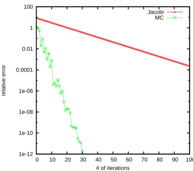
Figure 1 results for the relative error of the solution for the proposed algorithm and for the Jacobi method are presented.
One can observe that for the proposed WE Monte Carlo method the conver-gence is much faster and just after 30 iterations the solution is very accurate: the relative error is about 10−12. At the same time, the convergence of Jacobi
method is slower, and after 100 iterations the relative error is between 10−2
1e-12 1e-10 1e-08 1e-06 0.0001 0.01 1 100 0 10 20 30 40 50 60 70 80 90 100 relative error # of iterations Jacobi MC
Fig. 1. Relative error for the WE Monte Carlo for all components of the solution and Jacobi method for a matrix of size 5000 × 5000. The number of random trajectories for MC is 5n. 1e-12 1e-10 1e-08 1e-06 0.0001 0.01 1 100 0 10 20 30 40 50 60 70 80 90 100 relative error # of iterations Jacobi MC
Fig. 2. Relative error for the WE Monte Carlo for all components of the solution and Jacobi method for a matrix of size 25000 × 25000. The number of random trajectories for MC is 5n.
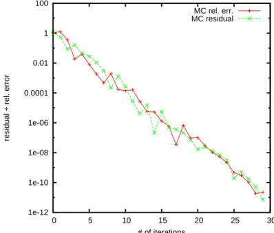
n = 25000. These results are shown on Figure 2. The results are similar. In order to see if the residual can be considered as a good measure for the error we compare the relative error with the residual for a matrix of size n = 5000
(see. Figure 3). One can observe that the curves presenting the relative error and the residual are very close to each other.
1e-12 1e-10 1e-08 1e-06 0.0001 0.01 1 100 0 5 10 15 20 25 30
residual + rel. error
# of iterations
MC rel. err. MC residual
Fig. 3. Comparison the relative error with the residual for the WE Monte Carlo 100 × 100. The number of random trajectories for MC is 5n.
5.2 Role of balancing for the quality of the algorithms
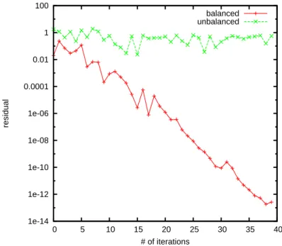
Let us mention that the balancing of matrices is a vary important issue for the deterministic algorithms. That is why for any arbitrary matrix a balancing procedure is needed as a preprocessing. Monte Carlo algorithms are not that sensitive to the balancing, but nevertheless, as it was shown in Subsection 3.3 the balancing affects the convergence of the WE Monte Carlo algorithm. The first example is shown on Figure 4 where we consider two matrices of small size n = 10. The balanced matrix is such that aij = 0.1, such that the parameter
a defined above is equal to 0.9. For the unbalanced matrix the parameter a is equal to 0.88, but the unbalanced matrix is extremity unbalanced (the ration between the largest and the smallest by modulo elements is equal to 40). Let us stress on the fact that this ratio is considered large when it is equal to 5.
The unbalanced matrix we deal with is the following:A=
0.4 0.4 0.01 . . . 0.01 0.01 0.4 0.4 . . . 0.01 . .. 0.4 0.01 0.01 . . . 0.4 .
Obviously, for the unbalanced matrix there is no convergence at all. For the balanced matrix the convergence is fast, but the red curve is rough. The reason
1e-14 1e-12 1e-10 1e-08 1e-06 0.0001 0.01 1 100 0 5 10 15 20 25 30 35 40 residual # of iterations balanced unbalanced
Fig. 4. Residual for the WE Monte Carlo for balanced and extremity unbalanced matrix of size n = 10. The number of random trajectories is N = 5n.
1e-14 1e-12 1e-10 1e-08 1e-06 0.0001 0.01 1 0 5 10 15 20 25 30 35 40 residual # of iterations balanced - # of rnd trajec. = 30 unbalanced - # of rnd trajec. = 500
Fig. 5. Residual for the WE Monte Carlo for balanced and extremity unbalanced matrix of size n = 10. The number of random trajectories for the balanced matrix is N = 5n; for the unbalanced matrix there two cases: (i) N = 5n – green curve; (ii) N = 50n – blue curve.
for that is that we use a very small number of random trajectories (N = 5n). Now we can consider the same matrices, but let us increase the number of the random trajectories to N = 500. At the same time we may decrease the number of the random trajectories (and also the computational time) from
N = 50 to N = 30 for the balanced matrix. The results of this numerical experiments are presented on Figure 5.
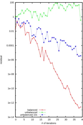
One can clearly see, that the WE algorithm starts to converge and after 35 to 40 iterations we have 3 correct digits. For the balanced matrix the convergence is still very fast, but again the red curve is rough, because of the small number of random trajectories. For a randomly generated matrices of size n = 5000 similar results are presented on Figure 6. The unbalanced matrix is generated by perturbing randomly the elements of the balanced matrix. The green and the blue curves correspond to the same unbalanced matrix, but the numerical results presented by the blue curve are obtained by using 10 times more ran-dom trajectories. In such a way, one can see that increasing the number N of random trajectories one can improve the convergence, as it is clear from the theory. In our particular numerical experiments shown on Figure 6 the green
1e-14 1e-12 1e-10 1e-08 1e-06 0.0001 0.01 1 100 0 5 10 15 20 25 30 35 40 residual # of iterations balanced unbalanced unbalanced 10x
Fig. 6. Residual for the WE Monte Carlo; the matrix of size is 5000 × 5000. The number of random trajectories for MC is 5n.
curve is obtained after a number of trajectories N = 5n, while the blue curve is based on N = 50n number of trajectories. One can see that in the first case the algorithm does not converge, while in the second case it converges. These experiments show that the WE Monte Carlo has another degree of freedom (which does not exist in deterministic algorithms) to improve the convergence even for very bad balanced matrices. The price we pay to improve the con-vergence is the increased complexity (or, the computational time) since we increase the number of simulation trajectories.
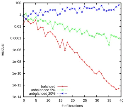
1e-14 1e-12 1e-10 1e-08 1e-06 0.0001 0.01 1 100 0 5 10 15 20 25 30 35 40 residual # of iterations balanced unbalanced 5% unbalanced 20%
Fig. 7. Residual for the WE Monte Carlo; the matrix of size is 100 × 100. Matrix elements are additionally perturbed by 5% and by 20%.
It is interesting to see how the disbanding affects the convergence of the WE Monte Carlo. We have performed the following numerical experiment: taking randomly generated matrices of differen size we were perturbing the matrix elements randomly by some percentage making the matrix more and more imbalanced. On Figure 7 we present the results for the matrix of size n = 100. The randomly generated entrances of the matrix are additionally perturbed by 5% and by 20%.
5.3 Comparison of WE with the preconditioned conjugant gradient (PCG) method
We compare our results with the optimal deterministic preconditioned con-jugant gradient (PCG) method [18,25,28]. Here is more precipe information about our implementation of the PCG method. We want to solve the linear system of equations Bx = b by means of the PCG iterative method. The in-put arguments are the matrix B, which in our case is the square large matrix N OS4 taken from the well-known Harwell-Boeing Collection. B should be symmetric and positive definite. In our implementation we use the following parameters:
• b is the right-hand side vector.
• tol is the required relative tolerance for the residual error, namely b − Bx. The iteration stops if ∥ b − Bx ∥≤ tol∗ ∥ b ∥.
• m = m1 ∗ m2 is the (left) preconditioning matrix, so that the iteration is (theoretically) equivalent to solving by PCG P x = m b, with P = m B. • x0 is the initial guess.
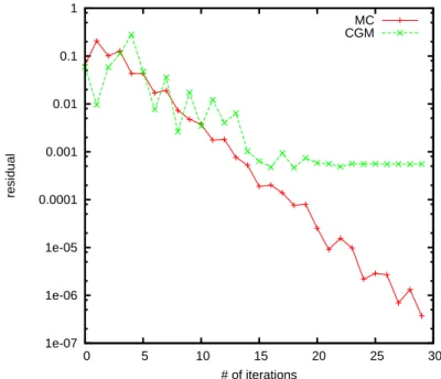
A comparison for convergency of the WE Monte Carlo and the PCG for the matrix N OS4 is presented in the Figure 8. This particular matrix is taken from an application connected to finite element approximation of a problem describing a beam structure in constructive mechanics [32].
1e-07 1e-06 1e-05 0.0001 0.001 0.01 0.1 1 0 5 10 15 20 25 30 residual # of iterations MC CGM
Fig. 8. Comparison of the WE Monte Carlo and the PCG method for a matrix N OS4 from the Harwell-Boeing Collection.
The results presented on Figure 8 show that the convergence for the WE Monte Carlo is better: the curve presenting the residual with the number of iterations is smoother and goes down to 10−6−10−7, while the curve presenting
the PCG achieves an accuracy of 10−3. Let us stress on the fact that for the
experiments presented the needed accuracy is set to tol = 10−8. One can not
guarantee that such an effect happens for every matrices, but there are cases in which the WE Monte Carlo performs better that the PCG.
6 Concluding remarks
A new Walk on Equations Monte Carlo algorithm for solving linear algebra problems is presented and studied. The algorithm can be used for evaluating all the components of the solution of systems. The algorithm can also be used to approximate the matrix inversion of square matrices. The WE Monte Carlo
is applied to real-valued, as well as to complex-valued matrices. It is proved that:
• the proposed random variable based on random walk on equations is an unbiased estimate of the solution vector;
• for the Monte Carlo estimator, the mean value of N realizations of the random variable, it is proven that the variance vanishes when N goes to infinity and converges almost surely to the solution;
• the structure of the relative stochastic error is analysed; it is shown that an interpolation Monte Carlo algorithm is possible for perfectly balanced matrices.
The analysis of the structure of the stochastic error shows that the rate of convergence of the proposed WE Monte Carlo algorithm depend on the bal-ancing of the matrix. This dependance is not that strong as for deterministic algorithms, but still exists.
A number of numerical experiments are performed. The analysis of the results show that:
• the proposed WE Monte Carlo algorithm combined with the sequential Monte Carlo for computing all the components of the solution converges much faster than some well-known deterministic iterative methods, like Ja-cobi method; this is true for matrices of different size and the effect is much bigger for larger matrices of size up to n = 25000;
• the balancing of matrices is still important for the convergency; many nu-merical results demonstrate that one should pay special attention to the balancing;
• the comparison of numerical results obtained by the WE Monte Carlo and the best optimal deterministic method, the preconditioned conjugant gra-dient, show that for some matrices WE Monte Carlo gives better results.
Acknowledgment
The research reported in this paper is partly supported by the European Commission under FP7 project AComIn (FP7 REGPOT-2012-2013-1, by the Bulgarian NSF Grant DCVP 02/1, as well as by the Universit´e du Sud Toulon-Var.
References
[1] V. Alexandrov, E. Atanassov, I. Dimov, Parallel Quasi-Monte Carlo Methods for Linear Algebra Problems, Monte Carlo Methods and Applications, Vol. 10, No. 3-4 (2004), pp. 213–219.
[2] Curtiss J.H., Monte Carlo methods for the iteration of linear operators, J. Math Phys., vol 32, No 4 (1954), pp.209–232.
[3] Curtiss J.H. A Theoretical Comparison of the Efficiencies of two classical methods and a Monte Carlo method for Computing one component of the solution of a set of Linear Algebraic Equations. ,Proc. Symposium on Monte Carlo Methods , John Wiley and Sons, 1956, pp.191–233.
[4] J. D. Densmore and E. W. Larsen, Variational variance reduction for particle transport eigenvalue calculations using Monte Carlo adjoint simulation, Journal of Computational Physics, Vol. 192, No 2 (2003), pp. 387–405.
[5] Dimov I. Minimization of the Probable Error for Some Monte Carlo methods. Proc. Int. Conf. on Mathematical Modeling and Scientific Computation, Albena, Bulgaria, Sofia, Publ. House of the Bulgarian Academy of Sciences, 1991, pp. 159–170.
[6] I. Dimov, Monte Carlo Algorithms for Linear Problems, Pliska (Studia Mathematica Bulgarica), Vol. 13 (2000), pp. 57–77. [7] I.T. Dimov, Monte Carlo Methods for Applied Scientists, New Jersey,
London, Singapore, World Scientific (2008), 291 p., ISBN-10 981-02-2329-3.
[8] I. Dimov, V. Alexandrov, A. Karaivanova, Parallel resolvent Monte Carlo algorithms for linear algebra problems, J. Mathematics and Computers in Simulation, Vol. 55 (2001), pp. 25–35.
[9] I.T. Dimov, B. Philippe, A. Karaivanova, and C. Weihrauch, Robustness and applicability of Markov chain Monte Carlo algorithms for eigenvalue problems, Applied Mathematical Modelling, Vol. 32 (2008) pp. 1511-1529.
[10] I. T. Dimov and A. N. Karaivanova, Iterative Monte Carlo algorithms for linear algebra problems, First Workshop on Numerical Analysis and Applications, Rousse, Bulgaria, June 24-27, 1996, in Numerical Analysis and Its Applications, Springer Lecture Notes in Computer Science, ser. 1196, pp. 150–160.
[11] I.T. Dimov, V. Alexandrov, A New Highly Convergent Monte Carlo Method for Matrix Computations, Mathematics and Computers in Simulation, Vol. 47 (1998), pp. 165–181.
[12] I. Dimov, A. Karaivanova, Parallel computations of eigenvalues based on a Monte Carlo approach, Journal of Monte Carlo Method and Applications, Vol. 4, Nu. 1, (1998), pp. 33–52.
[13] I. Dimov, A. Karaivanova, A Power Method with Monte Carlo Iterations, Recent Advances in Numerical Methods and Applications, (O. Iliev, M. Kaschiev, Bl. Sendov, P. Vassilevski, Eds., World Scientific, 1999, Singapore), pp. 239–247.
[14] I. Dimov, O. Tonev, Performance Analysis of Monte Carlo Algorithms for Some Models of Computer Architectures, International Youth Workshop on Monte Carlo Methods and Parallel Algorithms -Primorsko (Eds. Bl. Sendov, I. Dimov), World Scientific, Singapore, 1990, 91–95.
[15] I. Dimov, O. Tonev, Monte Carlo algorithms: performance analysis for some computer architectures, Journal of Computational and Applied Mathematics, Vol. 48 (1993), pp. 253–277.
[16] Forsythe G.E. and Leibler R.A. Matrix Inversion by a Monte Carlo Method, MTAC Vol.4 (1950), pp. 127–129.
[17] G. V. Golub, C. F. Van Loon, Matrix computations (3rd ed.), Johns Hopkins Univ. Press, Baltimore, 1996.
[18] Gene H. Golub and Q. Ye, Inexact Preconditioned Conjugate Gradient Method with Inner-Outer Iteration, SIAM Journal on Scientific Computing 21 (4): 1305. (1999). doi:10.1137/S1064827597323415. [19] J. Halton, Sequential Monte Carlo, Proceedings of the Cambridge
Philosophical Society, Vol. 58 (1962) pp. 57-78.
[20] J. Halton, Sequential Monte Carlo. University of Wisconsin, Madison, Mathematics Research Center Technical Summary Report No. 816 (1967) 38 pp.
[21] J. Halton and E. A. Zeidman, Monte Carlo integration with sequential stratification. University of Wisconsin, Madison, Computer Sciences Department Technical Report No. 61 (1969) 31 pp.
[22] J. Halton, Sequential Monte Carlo for linear systems - a practical summary, Monte Carlo Methods & Applications, 14 (2008) pp. 1–27.
[23] J.M. Hammersley, D.C. Handscomb, Monte Carlo methods, John Wiley & Sons, inc., New York, London, Sydney,Methuen, 1964. [24] L. W. Kantorovich and V. I. Krylov, Approximate Methods of Higher
Analysis, Interscience, New York, 1964.
[25] A.V. Knyazev and I. Lashuk, Steepest Descent and Conjugate Gradient Methods with Variable Preconditioning SIAM Journal on Matrix Analysis and Applications 29 (4): 1267, (2008). doi:10.1137/060675290
[26] S. Maire, Reducing variance using iterated control variates, Journal of Statistical Computation and Simulation, Vol. 73(1), pp. 1-29, 2003.
[27] N. Rosca, A new Monte Carlo estimator for systems of linear equations, Studia Univ. Babes–Bolyai, Mathematica, Vol. LI, Number 2, June 2006, pp. 97–107.
[28] Y. Saad, Iterative methods for sparse linear systems (2nd ed. – ed.). Philadelphia, Pa.: Society for Industrial and Applied Mathematics (2003) p. 195. ISBN 978-0-89871-534-7.
[29] I.M. Sobol Monte Carlo numerical methods, Nauka, Moscow, 1973. [30] J. Spanier and E. Gelbard, Monte Carlo Principles and Neutron
Transport Problem, Addison–Wesley, 1969.
[31] J.R. Westlake, A Handbook of Numerical matrix Inversion and Solution of Linear Equations, John Wiley & Sons, inc., New York, London, Sydney, 1968.
[32] Website: Matrix market, NOS4: Lanczos with partial reorthogonalization. Finite element approximation to a beam structure,