HAL Id: halshs-00639307
https://halshs.archives-ouvertes.fr/halshs-00639307v2
Submitted on 7 Apr 2014
HAL is a multi-disciplinary open access
archive for the deposit and dissemination of sci-entific research documents, whether they are pub-lished or not. The documents may come from teaching and research institutions in France or abroad, or from public or private research centers.
L’archive ouverte pluridisciplinaire HAL, est destinée au dépôt et à la diffusion de documents scientifiques de niveau recherche, publiés ou non, émanant des établissements d’enseignement et de recherche français ou étrangers, des laboratoires publics ou privés.
Unemployment Duration and Sport Participation
Charlotte Cabane
To cite this version:
Documents de Travail du
Centre d’Economie de la Sorbonne
Unemployment Duration and Sport Participation
Charlotte CABANE
2011.49R
Unemployment Duration and Sport Participation
∗
Charlotte Cabane
†November 2013
Abstract
In this study we use the German Socio-Economic Panel to evaluate the impact of leisure sport participation on the unemployment duration. The empirical litera-ture on sport participation has focused on labour market outcomes and job quality while the impact of this activity on job search has not been studied. However, sports participation fosters socialization which, through the networking effect, ac-celerates the exit from unemployment to employment. Furthermore, sporty people are expected to have valuable non-cognitive skills (self-confidence, persistence, team spirit). Last, they are healthier. These hypotheses are tested using survival analysis and taking into account unobservable heterogeneity. Because other activities could lead to similar positive effects we compare them to sporting activities and still find relevant results.
JEL Codes: J24, J64, L83
Keywords: Unemployment duration, Non-cognitive skills, Sport
∗we would like to thank Wladimir Andreff, Jean-Bernard Chatelain, Andrew Clark, Luke Haywood,
Yannick l’Horty, Rob Simmons, and the participants of the ESEA 5th
Conference, of the DAGStat conference, of the SSES conference, of the SIMA seminar, of the WIP seminar, of the DESport seminar, of the PSI-PSE seminar and of the SEW-HSG internal seminar for helpful comments and discussions.
†Swiss Institute for Empirical Economic Research - University of St. Gallen, Varnbuelstrasse 14
1
Introduction
It is most generally accepted that sporting activities are positive leisure activities. And, there is an increasing number of papers exhibiting a positive relationship between sports participation and educational success, health and success on the labour market. One specific situation on the labour market has been left behind: unemployment duration. And, for the same reasons that sporty people fare better on the labour market, we believe that these people experience shorter unemployment spells.
Sporting activities reduce unemployment duration...
First, sporty people have more cognitive and non-cognitive skills1 –such as tenacity,
self-confidence, competitive spirit, discipline– and thus their job search is more efficient which leads them to find a job quicker (and/or even a better job). Furthermore, many non-cognitive skills are a priori associated to people who declare practising one kind of sport. Therefore, even if they do not have these specific personal traits, it is assumed that they have it. And then whether it is true or not it represents additional information that can be used by the firm for the hiring process (selection of the candidate).
Second, sporty people are healthier which corresponds to a higher level of productivity but which is also often noticeable (visually speaking). Moreover, studies tend to show that there is beauty premium (Mobius & Rosenblat, 2006, Hamermesh & Biddle, 1994) and sport is often a way to modify ones figure.
And last but not least, participating into sporting activities is a way to socialize. Sporty people have larger and more diversified social networks and thus, they have relatively more opportunities than non-sporty people. Indeed, they have access to more information and benefit from more contacts and connections which could reduce the length of their unemployment spell. Bramoullé & Saint-Paul (2010) develop a dynamic model to explain why and how social networks influence labour market transitions.
1
Non-cognitive skills are personal preferences and personality traits which are valued in society but which do not involve technical or professional knowledge. Unlike cognitive skills, there is neither school nor diploma which allows learning and evaluating them.
Job status and social ties are interdependent and evolve through time. Bramoullé & Saint-Paul (2010) argue that the lower is the labour market turnover, the higher is the social segregation between employed and unemployed people. Therefore, individuals who have suffer from unemployment for a long time before being unemployed again experience lower exit rates from unemployment. And, people who stayed a long time employed before being unemployed experience higher exit rates from unemployment. These results are extremely interesting since they point out the fact that any activity which could connect unemployed people to employed people –such as sport practice– would partly break this time dependence / vicious circle.
... unless the context otherwise requires.
That being said, the effect of sports participation on unemployment duration is not straightforward. Unemployed people time use is highly sensitive. Indeed, time use to practise sport cannot be dedicated to job search. On one hand, if people do sport rather than looking for a job it mechanically increases their unemployment duration. But, if they do sport instead of watching TV and still look for a job for the same amount of time then it should not negatively impact the job search. On the other hand, firms could inter-pret sports participation2 as a negative signal indicating that the individual is not really
willing to work or to invest in her job. Bougard et al. (2011) demonstrate –in a recent experimental study performed on the French labour market– that job applicants who are involved in associations are significantly less often called than those who are not. Also, it is relevant to outline here the fact if unemployed people have more time and therefore, can invest more and in more activities, they have less income which reduces their access to some activities. Even if they receive benefits and enjoy discounted access to sports facil-ities, their options in terms of sports can be limited (i.e. some sports are more expensive).
The analysis of unemployment spell duration involves three periods: the first one t(u−1) during which the individual is employed or in education, the second one tu which
begins once she declares to be unemployed and the third one t(u+1) which begins when
2
she exits from unemployment to another situation.3 Mechanically, practising sports in
t(u+1) has no impact on the length of tu. Conversely, sport participation during tu signals
to firms that the individual is still physically active and thus healthy which is relevant with respect to her unobservable productivity at work. Moreover, it sends out a positive signal with respect to mental form too. A sporty unemployed individual is someone who does not give up -she is still socially active- once she is out of the labour market. Last, for unemployed as well as for employed people, it sends out information linked to the specific sport practised. A rugby player is seen as someone who has a great team spirit whereas a dancer is considered as very rigorous and well-disciplined, for example.
The efficiency of the networking effect depends on the reliability of the social network (Rees, 1966). Employed people are socially more attractive than unemployed ones and, they are in interaction with many more people. Capperalli & Tatsiramos (2010) study the impact of friends networks on job finding rate, wages and employment stability using data from the British Household Panel Survey (BHPS). Focusing on friends’ position on the labour market, they find out that having best friends employed increases the probability to find a job. Therefore, sporting activity as a socialization process is more effective for employed people. Furthermore, employed people can afford a broader range and more expensive sports than unemployed ones. This leads to more opportunities, to more interesting contacts (in terms of labour market opportunities) or even to meet people in a privileged environment (such as private clubs or facilities). Once the network is built, people have to maintain it by going on with sport participation even once they become unemployed.
Sports participation: a virtuous circle?
The literature outlines positive results of sports participation on education and labour-market outcomes. And individual’s labour market position influences in turn sports participation. As a result, it is less likely for sporty people to be unemployed. Therefore, the relevant question is whether people with different sports practice history
3
The individual can exit from unemployment to employment but also to retirement or to training or even leave the labour force.
can by practising sport while they are unemployed benefit from its positive effect on unemployment duration. For the aforementioned reasons we venture the hypothesis that being involved in sports decreases unemployment duration.
We use survival models to estimate the impact of weekly sports participation on unemployment duration. And, in order to define as precisely as possible the nature of this relationship, we use various specification and subsamples. Indeed, we need to reduce the selection on unobservables and also take into account the fact that the effect of sports participation can be heterogeneous. And, since other leisure activities could have similar effects as sporting activities, we test whether our effects are robust once we control for other activities. We find evidence that women who were not previously sporty and who practise sport weekly while they are unemployed spend less time unemployed. This is true for women having at least three years of work experience and women living in the former East Germany. Results are not that significant for men.
The article is organized as follows: in the next section we review the literature. The strategy of identification and the model used are presented in the third section. The fourth section is dedicated to the description of the data and the fifth section contains the results. We discuss our results and conclude in the last section.
2
Literature review
To our knowledge, there is no literature on the impact of sports participation on unemployment duration. And, most of the literature on the relationship between sport participation and labour market outcomes use North-American databases which consist of information on sporting practice during high school or college and labour market out-comes several years (10 to 13) later (Stevenson, 2010, Kosteas, 2012, 2011, Barron et al., 2000, Long & Caudill, 1991, Ewing, 1998). In this article we are interested in the con-temporary impact on sporting practice on individuals’ unemployment duration. Thereby, we put the emphasis on articles which study the immediate returns of sport participation.
Rooth (2011) demonstrated that indicating practising sports in the curriculum vitae does positively influence firms’ hiring process and decision to interview the candidate. A part of his analysis is based on an experimentation on the Swedish labour market. This kind of study is called testing or correspondence study and allows to measure the impact of individuals’ specific characteristics during the hiring process. Rooth (2011) found that people who declare practising sport as a leisure in their curriculum vitae have a higher probability of getting an interview. And, being sporty is equal to 1.5 additional years of work experience. He also estimates the impact of a variation of the physical fitness on earnings and finds a positive effect (4%). For this last impact it is harder to precise which effect is at work. Unlike the previous cited studies, Rooth (2011) is able to differentiate types of sports (football, fitness etc.). This is very important in order to pinpoint impacts.
Lechner (2009) uses the GSOEP and points out the positive relationship between sports participation and labour market outcomes. According to his study, being sporty is equal to an additional year of schooling in terms of labour market long-term outcomes. He identifies three channels: health, “mental health” and individuals’ unobservable characteristics. Sporty people are mentally and physically healthier thanks to sport par-ticipation.4 Therefore, they are more productive. Furthermore, they have unobservable
specific characteristics which match with unobservable characteristics held by people who earn more.
Beyond their specific socio-eco-demographic profile, Celse (2011) and Eber (2002) argue that sporty people behave differently. Both use experimental economics procedures to highlight traits specific to sporty people. Celse (2011) argues that sporty people suffer more from envy: they are very sensitive to social comparisons and tend to reduce others income in order to feel better. Another interesting result is that there are no differences between men and women when most studies outline gender specific results.5 Eber (2002)
4
Labour market outcomes depend on individuals’ productivity at work and a part of this productivity depends on health status. A healthy individual is less absent, more dynamic and more concentrated. By practising sports as an extracurricular activity, people maintain or increase their health status.
5
also runs an experiment6 and finds out that behaviours differ by gender: girls look more
for equality and boys look more for competition and these results are sharpened within sports science students. Both articles state that sporty people behave in a different way but they neither provide information on the reason of these differences nor identify a causal relationship.
Most of the studies which investigate the relationship between sport participation and labour market outcomes (or education returns) are done using American data. Knowing the role sports has in the USA (social promoter, integrator, etc.), one can fairly question the relevance of such type of analysis with respect to European countries. As a matter of fact, German data (mainly because of the availability of information on sports participation) have been used at least at three occurrences to investigate this topic. Two studies - Lechner (2009) and Pfeifer & Cornelißen (2010)- have been realized on the GSOEP (German Socio-Economic Panel) and both outlined a positive impact of sport participation on labour market outcomes and school returns. And, a study done by Felfe et al. (2011) highlight the existence of a positive influence of sports participation during childhood on cognitive and non-cognitive skills using a cross-section of German children from 3 to 10 years old (KiGGS). They insist on the advantages of sporting activities with respect to other leisure activities that are more passive (watching TV) and much less productive in terms of child development. In this paper we also use German data.
A last relevant segment of the literature that has been broadly studied is the determi-nants of sports participation. Severals studies analysis the determidetermi-nants of adults’ sports participation on the theoretical (Downward, 2007) and empirical side (Farrell & Shields, 2002, Downward, 2007, Hovemann & Wicker, 2009, Breuer, 2006, Breuer & Wicker, 2008, Humphreys & Ruseski, 2011) and highlight similar conclusions. Sporty people have al-most the same characteristics as successful people on the labour-market. Indeed, sports participation positively depends on the level of education and household income and
be-the same preferences, be-the distribution of men and women by type of sports would not be equal.
6
He confronts sports science students (STAPS) and average students to various hypothetical / fictive situations (the dictator game and a situation involving competition and gains comparison) and compares the results.
longing to ethnic minorities is negatively related to sport participation. Being older or less healthy is also negatively correlated to sports participation. The determinants that differ are the household characteristics and the marital status.7
3
Empirical framework
3.1
Identification strategy
The research question is: does being involved in weekly sports participation while being unemployed shorten unemployment duration? The observed population consists of people who experience unemployment during a specific time-window. We consider weekly sports participation during unemployment as a treatment. Therefore, the control group consists of people who are not sporty during the period of observation and the treated group is formed by people who are sporty while they are unemployed. The treatment is binary: practising sport weekly or less often. Unlike the ordinary/traditional treatment (such as unemployment benefits, formation/training) the exit from the original state (unemployment here) does not lead to the cessation of the treatment. Indeed, the individual decides to keep being treated (to practise sport) or not as she also decided to be treated in the first place. There is no third part involved in the choice of being treated. Therefore, by construction the treatment is not randomly assigned. This leads to two types of concerns: the selection on observables and the selection on unobservables.
We aim to remove the selection on observables by controlling for observable indi-viduals’ characteristics pre-treatment. We include in our estimation information on individuals’ situation on the labour market (regarding their last job), socio-economic status, familial situation, place of residence and health status. As we saw in the literature review, all the factors which impact labour-market outcomes are also determinants (and sometimes even outcomes) of sports participation. It is important to control for factors
7
Being married is negatively related to sport participation, the impact of the presence of children depends on individuals’ gender as well as on the age of the children. Indeed, the presence of infants in the household lowers adults sport participation while the presence of children increases the probability for men to practise sports.
which would influence unemployment duration as well as factors which would –through sports participation– impact the duration. The introduction of the latter (mediators: characteristics which affect unemployment duration via sports participation) can lead to reduce the overall impact of sports participation. Indeed, sports participation is positively determined by health which also depends on sports participation. Therefore, by controlling for the health status for example, we mechanically remove the health effect of sports participation which leads to undervalue the size of the effect. For this reason, we will successively add and remove each potential mediator in order to be able to characterize the relationship.
The selection on unobservables is –as often– harder to neutralise. We proceed in two steps. First, we build different subsamples. Sporty people are different to not sporty people in many ways and also, the past sports participation is an important determinant of current participation. Therefore, we divide our sample according to the individuals’ sports participation history before being unemployed. Estimating the relation for these different subsamples separately allows us to only compare people of the same type: sporty people among themselves and not sporty people among themselves. Given that sports participation is highly correlated with labour-market situation, we believe that by doing this we remove a significant part of the selection due to unobservables. However, it might be that there are still unobservable confounders within our subsamples. We cannot reasonably divide again our subsamples due to sample size issues therefore, in a second step, we include shared frailty which is equivalent to adding random effect in our estimations. And, since we have in most of the cases more than one unemployment spell by individual, by using this additional information we believe we can reduce a significant part of the endogeneity
Another concern is that the effect could be heterogeneous among individuals. Since the model used is not linear, the use and then the interpretation of interaction terms is complicated. This is why we decided to estimate the effect on different subsample (within our original subsamples). First of all, we expect the effect to differ by gender.
Men and women do not practise the same type of sports. Men are more likely to do team sports and women individual sports. And, this differences lead to a different type of participation all over the life cycle. Indeed, women sports participation is more constant than men sports participation. And, men and women labour-market opportunities are often different. We therefore always run estimations by gender. Second, since the sports culture as well as the labour-market situation is significantly different in former East Germany and former West Germany, we look at the results within these two geographical entities. Last, if we consider sports participation as a signal its impact might depend on individual’s length of work experience. Indeed, signals are used when firms cannot directly measure individuals’ productivity. This means that the relevance of the signal depends on the availability of other information such as work experience. Therefore, the importance of sport participation impact on the exit rate should be greater for inexperi-enced/young people.8 And, since we introduce a measure of the health, we control for this part of individuals’ productivity which also vary with age. We test the relationship on various sub-samples built with respect to a specific number of years of work experience.
One can signal specific non-cognitive skills and enlarge social networks by being in-volved in volunteering for example. In order to check the specificity of sporting activities, we build different treatment associated to the following activities: taking part in vol-untary work and being a churchgoer.9 The comparison of these different treatments in
terms of activities allows defining more precisely the kind of observed relationship and the channels at work.10 These two activities(as well as sports participation) are related
to socialization and networks. Therefore, the impact of sports participation should be lower or even disappear once these two activities are included in the estimates. They all are composed of a substantial cultural part: religion, political views or hobby. Therefore, besides the social aspect of being with friends (or at least within a network), they also
8
They have spent less time on the labour market thus, the amount of information available with respect to their level of productivity is relatively low.
9
These are the activities available in the GSOEP questionnaire. A third one is actually proposed: "participating in local politics" but there is two few people taking part in it in our sample. Therefore, we leave it out and focus on the two activities mentioned in the core of the text.
10
The strategy remains the same thus, the control group consists in people who were not involved in the specific activity before and who still do not practise it once they are unemployed.
relates to a specific kind of culture. They are all practised weekly but being a volunteer often implies a stronger commitment –in terms of time resources and investment– than being churchgoer. 11 Furthermore, volunteering can be specified in one’s CV and thus
be used by the firm as additional information on the individual’s personal traits. The culture and personal traits conveyed by sporting activities are different in a sense that they do not involved personal or political view and believes. Therefore, it is interesting to compare the impact of these two activities on unemployment duration in order to precise the role played by sporting activities.
3.2
Survival models
We study unemployment duration and thus use survival analysis.12 Since the information
on labour-market situation is monthly recorded we have intervals rather than continuous time therefore, we use a discrete time survival model.13
We use a parametric model assuming a proportional relationship between the baseline hazard and the influence of individuals’ characteristics.14 For the proportional hazard
model, the hazard rate at time t for the subject i is written as follows:
h(t|xi) = h0(t)ϕ(Xi, βx) (1)
with the systemic part of the hazard rate for the subject i
ϕ(Xi, βx) = exp(Xiβx)
The probability of transiting from unemployment to employment in t for the individual i (1) is the product of the baseline hazard h0(t) and her individual characteristics Xi.
The baseline hazard is the probability for everyone in the sample to exit at the time
11
Indeed, people rely on volunteers whereas being churchgoer can be somehow considered as an indi-vidual activity in the sense that the religious event weakly depends on the indiindi-vidual participation.
12
In order to get to know this type of model we read Van den Berg (2001) and Jenkins (2004) which are very comprehensive writings on that topic.
13
In the models used in this article, the unemployment spell are allowed to be right censored in order to be considered.
14
Our sample is not large enough to allow us to use non-parametric models which requires a huge number of observations in order to be estimated.
t, knowing they survived (they stayed unemployed) until time t − 1. The sample is assumed to be homogeneous with respect to this baseline hazard. The proportionality of the hazard means that, for every individuals, the impact of x years of schooling is βyearsof schooling∗ h0(t), for example. Individuals who have an x twice bigger automatically
have a probability of exit twice bigger (ceteris paribus). In other words, the shape of the survival function remains the same and only its level changes.
A large part of our sample experiences more than one unemployment spell over the period (25 years). Unobservable characteristics which influence the risk of getting unemployed must be taken into account. In fact, forgetting to consider it leads to overestimate (underestimate) the degree of negative (positive) duration dependence. Individuals (observations) with a high level of frailty -which means unobservable charac-teristics which increase their chances to find a job- get out faster from unemployment. Therefore, there are within the survivors more individuals with a low level of frailty and this proportion increases with time. Because the level of frailty is unobserved, the impact of this selection is directly imputed to time. In other words, the influence of t being over-estimated, the impact of the covariates is mechanically under-estimated.
A way to adress this problem is to introduce individual frailty modeled as a parameter α which is normally distributed.15 The belonging of a duration to a group is estimated
and not specified ex-ante. The unobserved characteristics are assumed to be independent from the covariates which comes to add individuals’ random effect in the model. The hazard ratio is thus written as follows:
h(t|xij) = h0(t)αjϕ(Xi, βx) (2)
αj being the group-level frailty (here a group j is an individual and i is an observation),
αj > 0 and αj ∼ N (m, σ2).
15
It would have been interested to use also Heckman and Singer semi-parametric frailty (Heckman & Singer, 1984) which allows taking into account heterogeneity without giving any functional form to the distribution of unobservables. However, as mentioned before our sample is too small to run successfully non-parametric estimation given that we also have a large number of covariates.
For νj = log αj, the hazard can be written as follows:
h(t|xij) = h0(t) exp(Xiβx+ νj)
Shared frailty can be introduced for the whole sample, however, in presence of within cluster correlation, the standard errors are incorrect. Therefore, in order to avoid this risk we run the estimates on a restricted sub-sample (but we also present results obtained for the whole sample in order to get an idea of the selection and more information on the mechanisms).
The complementary log log specification allows for a discrete representation of a con-tinuous time proportional hazards model. The idea being that we do not know the exact survival time but we know the interval of time in which it occurs (a month in our data). The interval hazard rate h(aj) (also called discrete hazard rate (aj−1, aj]) can be expressed
as follow:
h(aj) = P r(aj−1 < T ≤ aj|T > aj − 1) = 1 − (S(aj)/S(aj−1))
Once taken into account the specific form of the survival funtion we can rewrite h(aj)
the discrete hazard rate (aj−1, aj] as follow:
h(aj, X) = 1 − exp[− exp(β′X + γj)]
with γj = log[− log(1 − h0j)]
cloglog[h(j, X)] = D(j) + β′
X
with D(j) the baseline hazard function. Which, including shared frailty ν (νj = log αj)
leads to this expression:
cloglog[h(j, X)] = D(j) + β′
4
Data
We use the German Socio Economic Panel (GSOEP). The panel runs from 1984 until nowadays and contains around 20’000 individuals by wave. There are various yearly questionnaires which enable to have a great definition of the individuals’ current and past situation. Labour market information is recorded monthly which allows us to use survival models. However, individuals’ characteristics are recorded yearly and information about sports is asked even less frequently.
4.1
Construction of the samples
We build subsamples according to sports participation history of the individuals and then within the different groups we define the treatment. The treatment is always "practising sports at least weekly while being unemployed". Individuals are questioned about their sport practice frequency every two years except between 1994 and 1999. In this interval the information is available each year. The question is the following:
How frequently do you do sports? – once per week,
– once per month,
– less than once per month, – never.
There is no formal definition of what the interviewer understands by doing sports16
thus, there is a risk of measurement error. Actually, 17% of the population sampled declares to practice a physical activity at least once a week. This figure is below national statistics about sport participation in Germany but it is thus coherent knowing that it concerns only people who experience unemployment (sample in which sporty people are under-represented). Besides, since it is self-declared and being sporty is positively looked upon, people have an incitation to lie about their sporting activity. But the figures size being reasonable, it leads to be more confident with respect to this information.
16
We distinguish three different types of people: the sporty people, the not sporty people and the inactive people. Each group is defined as followed:
* Sporty: people who practised sports weekly17 during the two years precedent the unemployment spell.18 Treatment: Continue with weekly sports participation while
being unemployed.
* Not sporty: people who practised sports less than weekly during the two years precedent the unemployment spell. Treatment: Begin to practise sports weekly while being unemployed.
* Inactive: people who practised all the activities (volunteering and being a church-goer) less than weekly during the two years precedent the unemployment spell. Treatment: Begin to practise sports weekly while being unemployed.19
As mentioned above, with respect to sporting activities during the unemployment spell the treatment is similar for all the subsamples. Indeed, we can define in all subsamples the control group as people who do not do sports or less than weekly and the treated group as people who practise sports weekly.
Unemployment duration can last less than a year and exit can occur before the survey interview for the current year. And labour-market position highly impacts sports partic-ipation (budget constraints, time constraints). Therefore, it is relevant to deal with the potential time inconsistency issue due to timing event and data collection. We choose to keep only the observations that have been collected the same month when unemployment begins or in between entry and exit from unemployment.
Example: individual i is unemployed between January and March 93, indi-vidual j is unemployed between March and June 93 and indiindi-vidual k is
un-17
Definition coherent with the European standard.
18
Since the question is not asked every year we impute the value of the variable considering that the sports behaviour is equivalent to the sports participation the year before and the year after the missing observation. If the participation is different we use the level of participation of the precedent year. Since we define the profile of an individual by relying on the information over the two last years precedent unemployment we have at least one observation which is really observed (ie. not imputed).
19
There is an overlap of the not sporty and inactive sample. Indeed, the inactive subsample being the most restrictive in terms of definition, some inactive people are included in the not sporty sample.
employed since May 93. If the interview have been conducted in April 93 we use only the observations of individual j. Indeed, i has given information on his personal situation after her exit from unemployment thus it is not relevant and k answer to the survey while she was employed (or at least not unem-ployed) so we cannot infer that she did not change her behaviour/activity participation once she enters unemployment on month later in 1993.
We proceed the same way with respect to the other activities that we test. The formulation of the question is the following: How frequently do you volunteer work in clubs, associations, or social services? and, How frequently do you go to church or religious institutions? As for sporting activities we consider an individual as treated (ie. an individual who is newly frequently involved) in such activities if she answers participating at least weekly in it.
We focus on transitions from unemployment to either full-time or part-time employ-ment. Temporary jobs, apprenticeships, formation etc. are not considered as an exit from unemployment. Therefore, the transitions we are looking at are supposed to be "real ex-its" from unemployment. The sample is restricted to people who: i) become unemployed for at least a month between 1984 and 2009 and ii) are between 17 and 45 years old when they become unemployed. The age is limited to 45 years old since older people that are closer to the retirement age might have very different strategies in terms of job search and exiting unemployment.
4.2
Descriptive statistics
The covariates used in the estimation are: the level and type of education (using the casmin classification), the familial status, the number of children up to 14 years old, the number of children between 15 and 18 years old, the age, the age squared, the nationality (German or not), the sex, the level of health satisfaction,20 the total number
of the individual’s unemployment spells and the number of the current one, the work
20
The variable health satisf action is a discrete variable equal to 0 if the individual is extremely dissatisfied by her health and equal to 10 if she is extremely satisfied. The information is much more often given by the respondent than the one concerning the health status.
experience, the unemployment experience and the labour net income from the last year as well as the number of working hours and the size of the firm (before the unemployment spell starts). Individuals’ characteristics which can change over time and influence the exit from unemployment are taken 12 months before the entry in unemployment. Then, in order to take into account the individual specific economic environnement in terms of time and location we add the years and the Land of residence. The time is added as seven intervals of different numbers of months: up to 3 months, 3 to 6 months, 6 to 9 months, 9 to 12 months, 12 to 18 months, 18 to 24 months and more than 24 months.
The comparison of the control and the treated group with respect to the covariates is informative in terms of potential selection effect and confirms the literature prediction (descriptive statistics are reported in Table 1 for women and Table 2 for men). The number of observations is here the number of spells, there are 1805 individuals in total. The treated are unemployed for shorter periods. They are more likely to be German, they are almost two years younger in average. They have in average a higher level of education and are more often involved in volunteering. And, as expected, they are more satisfied with their health. In terms of labour-market situation, treated people are better off than the control group. Indeed, they experiment less unemployment spells and exit more often from unemployment to employment. Last but not least, it is interesting to notice that the sporty samples (for men and women) are more homogeneous than the other subsamples when comparing controls and treated. It is not surprising given that the treatment for sporty people does not mean getting newly involved in sport but rather continuing with being actively sporty.
5
Results
The Table 3 shows the baseline estimations of the impact of weekly sports participation on the exit rate from unemployment to employment using the complementary log log model within each subsamples. Results are different by gender and it is worth noticing that the introduction of the frailty is not necessary in each subsamples. As we saw
before, the sporty subsamples are more likely to be homogeneous and therefore, do not need the introduction of shared frailty whereas the other subsamples do.21 Also, the
results of the estimates including shared frailty have to be interpreted knowing that each individual has a fixed νi (i.e. individuals’ level of frailty).22
The coefficient associated to the treatment – practising sports at least weekly– is positive and significatively different from zero only for not sporty or inactive women. This means that a priori they are the only ones who could benefit from beginning to be sporty once they are unemployed. The coefficients are large but smaller than the ones associated to education and elapsed time which makes it reasonable. For the men subsamples, the effect is not significantly different from zero.
5.1
Women samples
We did not report the results of the mediation analysis for a sake of clarity.23 But,
thanks to this analysis we found out that even once we remove all the covariates that could supposedly be linked to sports participation,24 the treatment still appears
to be uncorrelated to the exit rate for sporty people. In the not sporty and the inactive subsamples this procedure leads to an important increase of the size of the coefficient associated to the weekly sports participation (multiplied by 1.5). However, it is interesting to notice that, in all the subsamples, the coefficients associated to the educational variables do increase once we remove the weekly sports participation from the set of covariates. This leads us to consider education as a mediator.
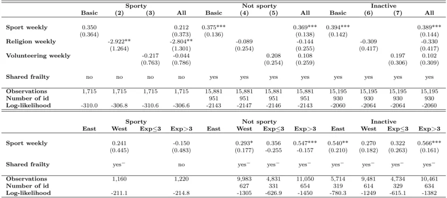
The results of the other specifications we run are available in Table 4. The first part of the table shows the results of the beauty contest in each subsample. In a first step,
21
Each estimation has initially been run using shared frailty, and regressions which do not need the frailty (ie. the likelihood-ratio test indicates that θ –the frailty variance– is not significantly different from 0) have been re-run without.
22
Results are conditional on this level.
23
The results are available upon request.
24
Namely: the educational levels and types, the number of children, the status in the household, the work experience, the number of unemployment spells, the health satisfaction and the past labour-market position.
we run a “beauty contest” in order to find out which activity is the most efficient (the reference being the sporting activity) with respect to transitions from unemployment to employment. Using the complementary log log model including shared frailty (except in the sporty sample), we compare the log likelihood among each estimation but differences are negligible. A first look at the figures allows seeing that results concerning the relation between weekly sports participation and exit from unemployment to employment are stable. Indeed, there is no impact in the sporty sample but there is a sizeable and significant correlation within the not sporty and inactive individuals even once controlling for weekly participation to other activities. In these two subsamples volunteering or being a churchgoer appears not to be correlated at all with exit from unemployment. In other words, since the impact of sporting activities on unemployment duration is not affected by a participation to other activities it confirms the specificity of sports in terms of returns. In the sporty sample, the exit rate seems to be negatively affected by being a churchgoer.
The second part of the Table 4 shows the results obtained when we divide our subsam-ples according to the region of residence and the years of work experience.25 It turns out
that the significant positive impact of weekly sports participation concerns exclusively inactive or not sporty women who have at least three years of work experience. Similarly, when we divide the subsamples by region of residence one can see that the impact is sig-nificantly different from zero (and sizable) for women living in the former East Germany but not for women leaving in the former West Germany.
5.2
Men samples
The mediator analysis on the male subsamples generates interesting results. For the not sporty as well as for the inactive subsample using or not the variable "weekly sports participation" does not make any difference in terms of size and significance of the coefficients of the (other) variables and also in terms of log likelihood. However, when all
25
Due to very reduced sample sizes we could not run our estimations for sporty and not sporty women living in the former East Germany and also for sporty women having less or up to three years of work experience.
the potential mediators are removed in the estimation on sporty people then our variable of interest appears to be highly positively and significantly correlated to the exit rate from unemployment to employment in t. This means that sporting activities per se do not affect the exit rate. It serves as a proxy when relevant controls (such as education, health, work experience) are missing.
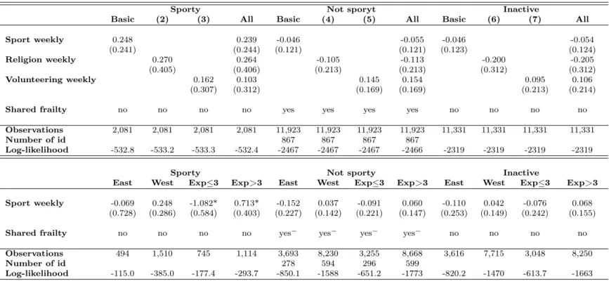
The Table 5 shows the detailed results of the others estimations we run. As expected, weekly sports participation does not impact the exit rate in any of the subsamples even once we add other activities to the estimation. However, it is interesting to notice that none of the tested activities matters.
The division of the subsamples by region of residence seems to confirm that weekly sports participation is not related to exit rate from unemployment for men (sporty, not sporty or inactive men). But the estimation by level of work experience does reveal a very interesting fact: weekly sports participation is positively correlated with an increase in the exit rate from unemployment for sporty men who have at least three years of work experience. On the contrary, practising sports weekly for sporty men who have less than three years of work experience appears to decrease the probability of exiting unemployment for employment in t. Levels of significance are lower but it is still interesting to see that relations are going in opposite senses once we divide the sample.
6
Discussion & Conclusion
Weekly sports participation is related to a quicker exit from unemployment to employ-ment for specific subsamples. However, since the treatemploy-ment mainly works for people who were actually inactive or not-sporty until being unemployed (at least 2 years before over the period) we do not expect the treatment to affect consistently the individuals’ characterisitics. Moreover, the majority of the individuals spend less than a year unemployed meaning that the duration of the treatment is rather short. Therefore,
we cannot invoke the following traditional channels: networking effect (too little time to build a reliable network), health effect, skills creation or signaling effect (too short practice to mention it on a CV).
However, our effects are significant and sizeable even once we reduce as much as possible the selection on unobservables. And, this effect does not disappear when we control for being involved in volunteering or being churchgoer. Therefore, we believe that our variable of interest captures a state of mind: people who choose to take advantage of being unemployed to spend time practising sport might be in a better state of mind with respect to job search and labour-market re-integration than people who decide not to be sporty. As suggested by Caliendo et al. (2010), individuals’ mental predisposition is relevant for job search. And, there is no such an impact of volunteering because the investment is different, somehow heavier. Doing sport does not involved less social investment than volunteering. This is also consistent with the fact that we find different results for each sex and by level of work experience. Indeed, the level of motivation or the state of mind of new labour market entrants is different than the one of more experienced (and more likely older) workers.
References
Barron, John M., Ewing, Bradley T., & Waddell, Glen R. 2000. The Effects Of High School Athletic Participation On Education And Labor Market Outcomes. Review of Economics and Statistics, 82(3), 409–421.
Bougard, Jonathan, Brodaty, Thomas, Emond, Celine, L’Horty, Yannick, Parquet, Loïc Du, & Petit, Pascale. 2011. Les effets du bénévolat sur l’accès à l’emploi: une expérience contrôlée sur des jeunes qualifiés d’île de France. Tech. rept.
Bramoullé, Yann, & Saint-Paul, Gilles. 2010. Social networks and labor market transi-tions. Labour Economics, 17, 188–195.
Breuer, Christoph. 2006. Sportpartizicaption in Deutschland - ein demo-ökonomisches Modell. Discussion Paper. DIW Berlin.
Breuer, Christoph, & Wicker, Pamela. 2008. Demographic and economic factors influenc-ing inclusion in the German sport system - a microanalysis of the years 1985 to 2005. European Journal for Sport and Society, 5(1), 35–43.
Caliendo, Marco, Cobb-Clark, Deborah A., & Uhlendorff, Arne. 2010. Locus of Control and Job Search Strategies.
Capperalli, Lorenzo, & Tatsiramos, Konstantinos. 2010. Friends’ Networks and Job Find-ing Rates. IZA DP. IZA.
Celse, Jérémy. 2011. Damaging the perfect image of athletes; How sport promotes envy. Document de Recherche. LAMETA - Laboratoire Montpelliérain d’Economie Théorique et Appliquée.
Downward, Paul. 2007. Exploring the Economic Choice to Participate in Sport: Results from the 2002 General Household Survey. International Review of Applied Economics, 21(5), 633–653.
Eber, Nicolas. 2002. La pratique sportive comme facteur de capital humain. Revue juridique et économique du sport, 65, 55–68.
Ewing, Bradley T. 1998. Athletes and work. Economics Letters, 59(1), 113–117.
Farrell, Lisa, & Shields, Michael A. 2002. Investigating the economic and demographic determinants of sporting participation in England. Journal of the Royal Statistical Society Series A, 165(2), 335–348.
Felfe, Christina, Lechner, Michael, & Steinmayr, Andreas. 2011. Sports and Child De-velopment. CEPR Discussion Paper No. 8523.
Hamermesh, Daniel S, & Biddle, Jeff E. 1994. Beauty and the Labor Market. American Economic Review, 84(5), 1174–94.
Heckman, James, & Singer, Burton. 1984. A Method for Minimizing the Impact of Distributional Assumptions in Econometric Models for Duration Data. Econometrica, 52, 271–320.
Hovemann, Gregor, & Wicker, Pamela. 2009. Determinants of sport participation in the European Union. European Journal for Sport and Society, 6(1), 49–57.
Humphreys, Brad, & Ruseski, Jane. 2011. An Economic Analysis of Participation and Time Spent in Physical Activity. The B.E. Journal of Economic Analysis & Policy, 11(1).
Jenkins, Stephen P. 2004. Survival Analysis. Unpublished manuscript, Institute for Social and Economic Research, University of Essex, Colchester, UK.
Kosteas, Vasilios D. 2011. High School Clubs Participation and Future Supervisory Sta-tus. British Journal of Industrial Relations, 49(s1), 181–206.
Kosteas, Vasilios D. 2012. The Effect of Exercise on Earnings: Evidence from the NLSY. Journal of Labor Research, 33(2), 225–250.
Lechner, Michael. 2009. Long-run labour market and health effects of individual sports activities. Journal of Health Economics, 28(4), 839–854.
Long, James E., & Caudill, Steven B. 1991. The impact of Participation in Intercollegiate Athletics on Income and Graduation. Review of Economics and Statistics, 73(3), 525– 531.
Mobius, Markus M., & Rosenblat, Tanya S. 2006. Why Beauty Matters. American Economic Review, 96(1), 222–235.
Pfeifer, Christian, & Cornelißen, Thomas. 2010. The impact of participation in sports on educational attainment–New evidence from Germany. Economics of Education Review, 29(1), 94–103.
Rees, Albert. 1966. Information Networks in Labor Markets. American Economic Review, 56, 556–566.
Rooth, Dan Olof. 2011. Work Out or Out of Work: The Labor Market Return to Physical Fitness and Leisure Sport Activities. Labour Economics, 18(3), 399–409.
Stevenson, Betsey. 2010. Beyond the Classroom: Using Title IX to Measure the Return to High School Sports. Review of Economics and Statistics, 92(2), 284–301.
Van den Berg, Gerard J. 2001. Duration models: specification, identification and multi-ple durations. Chap. 55, pages 3381–3460 of: Heckman, J.J., & Leamer, E.E. (eds), Handbook of Econometrics. Handbook of Econometrics, vol. 5. Elsevier.
Table 1: Descriptive statistics - Women subsamples
Sporty Not sporty Inactive
Mean Mean Mean
Min Max Control Treated Diff Control Treated Diff Control Treated Diff
Covariates Age 19 54 32.60 32.67 34.30 32.89 *** 34.05 32.62 *** German 0 1 0.82 0.90 *** 0.81 0.91 *** 0.81 0.92 *** East 0 1 0.28 0.29 0.37 0.33 *** 0.37 0.33 *** Health sat. 0 10 6.89 6.75 *** 6.51 6.62 *** 6.47 6.58 *** Head hh. 0 1 0.65 0.67 0.54 0.59 *** 0.55 0.59 ***
Nb. of children 15 to 18 years old 0 3 0.27 0.23 0.29 0.26 ** 0.30 0.27 **
Nb. of children up to 14 years old 0 8 0.75 0.75 1.20 1.03 *** 1.18 0.99 ***
Religion weekly 0 1 0.05 0.05 0.05 0.08 *** 0.02 0.03 ***
Volunteering weekly 0 1 0.04 0.09 *** 0.02 0.12 *** 0.01 0.09 ***
Gal. Elementary sch. 0 1 0.20 0.08 ** 0.19 0.17 * 0.20 0.19
Basic Voc. Qual. 0 1 0.24 0.19 ** 0.22 0.14 *** 0.22 0.16 ***
Intermediate Gal. Qual. 0 1 0.03 0.01 ** 0.07 0.09 *** 0.07 0.09 ***
Intermediate Voc. 0 1 0.32 0.48 *** 0.33 0.34 0.33 0.34
Gal. Maturity Certificate 0 1 0.03 0.01 *** 0.01 0.00 *** 0.01 0.00 ***
Voc. Maturity Certificate 0 1 0.03 0.06 *** 0.03 0.05 *** 0.03 0.06 ***
Lower Tertiary Educ. 0 1 0.02 0.03 0.01 0.06 *** 0.01 0.05 ***
Higher Tertiary Educ. 0 1 0.10 0.10 0.05 0.13 *** 0.05 0.11 ***
Firm size (last job) 0 11 2.97 2.30 *** 2.58 2.39 ** 2.61 2.38 **
Working hours (last job) 0 70 15.70 12.07 *** 13.05 12.83 13.14 13.09
Net labour income (last job) 0 5900 369.50 326.36 * 268.63 286.14 270.10 283.91
Work exp. full time 0 27.5 4.35 4.95 ** 6.22 4.84 *** 6.17 5.02 ***
Work exp. part time 0 24.2 3.06 2.35 *** 1.71 2.23 *** 1.67 1.99 ***
Unemp. exp. 0 19.2 2.36 3.08 *** 3.06 2.33 *** 3.05 2.34 ***
Current u. spell num. 1 22 2.31 2.57 *** 2.22 2.44 *** 2.25 2.46 ***
Total nb. of u. spells 1 23 3.21 3.69 *** 2.92 3.11 *** 2.97 3.14 ***
Time
Unemp. spell: 1-6 months 0 1 0.26 0.23 0.17 0.23 *** 0.17 0.23 ***
Unemp. spell: 3-6 months 0 1 0.21 0.17 * 0.15 0.18 *** 0.15 0.18 **
Unemp. spell: 6-9 months 0 1 0.14 0.12 0.12 0.14 * 0.12 0.13
Unemp. spell: 9-12 months 0 1 0.09 0.09 0.10 0.10 0.10 0.10
Unemp. spell: 12-18 months 0 1 0.11 0.09 0.11 0.10 * 0.11 0.09 **
Unemp. spell: 18-24 months 0 1 0.07 0.06 0.09 0.07 *** 0.08 0.07 **
Unemp. spell: sup. 24 months 0 1 0.12 0.23 *** 0.27 0.19 *** 0.26 0.20 ***
Unemp.: nb. of months 1 145 11.03 18.54 *** 18.69 14.16 *** 18.42 14.65 ***
Nb. Obs. 576 1268 14322 1566 13466 1436
Notes: * significant at 10%; ** significant at 5%; *** significant at 1%.
25 Documents de Travail du Centre d'Economie de la
Table 2: Descriptive statistics - Men subsamples
Sporty Not sporty Inactive
Mean Mean Mean
Min Max Control Treated Diff Control Treated Diff Control Treated Diff
Covariates Age 19 56 30.76 28.74 *** 34.55 31.35 *** 34.53 31.20 *** German 0 1 0.77 0.79 0.75 0.78 ** 0.75 0.79 *** East 0 1 0.20 0.30 *** 0.31 0.22 *** 0.32 0.22 *** Health sat. 0 10 7.23 7.23 *** 6.11 6.64 *** 6.09 6.67 *** Head hh. 0 1 0.46 0.47 0.60 0.51 *** 0.61 0.50 ***
Nb. of children 15 to 18 years old 0 3 0.19 0.24 ** 0.26 0.28 * 0.25 0.28 **
Nb. of children up to 14 years old 0 7 0.57 0.46 ** 0.78 0.68 *** 0.76 0.66 ***
Religion weekly 0 1 0.08 0.06 0.07 0.04 *** 0.03 0.02 *
Volunteering weekly 0 1 0.01 0.13 *** 0.04 0.07 *** 0.02 0.06 ***
Gal. Elementary sch. 0 1 0.25 0.13 *** 0.23 0.24 0.22 0.24
Basic Voc. Qual. 0 1 0.29 0.28 0.30 0.35 *** 0.29 0.34 ***
Intermediate Gal. Qual. 0 1 0.05 0.08 *** 0.09 0.06 *** 0.09 0.06 ***
Intermediate Voc. 0 1 0.15 0.22 *** 0.22 0.18 *** 0.23 0.18 ***
Gal. Maturity Certificate 0 1 0.06 0.06 0.01 0.05 *** 0.01 0.05 ***
Voc. Maturity Certificate 0 1 0.08 0.07 0.04 0.06 *** 0.04 0.06 ***
Lower Tertiary Educ. 0 1 0.04 0.03 * 0.01 0.00 *** 0.01 0.00 ***
Higher Tertiary Educ. 0 1 0.04 0.07 ** 0.03 0.03 0.03 0.03
Size of the firm (last job) 0 11 3.59 4.16 *** 3.54 3.80 ** 3.52 3.69
Working hours (last job) 0 80 23.27 22.61 22.53 22.48 22.30 22.01
Net labour income (last job) 0 3250 527.32 532.53 539.02 571.60 * 538.16 551.78
Work exp. full time 0 29 6.36 4.90 *** 9.69 6.79 *** 9.80 6.61 ***
Work exp. part time 0 19 0.71 0.55 ** 0.58 0.71 *** 0.51 0.70 ***
Unem. exp. 0 19.9 2.40 1.84 *** 3.64 2.72 *** 3.55 2.76 ***
Current u. spell num. 1 20 2.35 2.58 *** 2.66 2.55 * 2.64 2.57
Total nb. of u. spells 1 20 3.05 3.82 *** 3.66 3.58 3.64 3.61
Time
Unemp. spell: 1-3 months 0 1 0.25 0.34 *** 0.22 0.24 ** 0.22 0.24 *
Unemp. spell: 3-6 months 0 1 0.21 0.22 0.15 0.17 * 0.15 0.17 **
Unemp. spell: 6-9 months 0 1 0.15 0.13 0.10 0.11 0.10 0.11
Unemp. spell: 9-12 months 0 1 0.10 0.08 ** 0.07 0.09 0.08 0.09 **
Unemp. spell: 12-18 months 0 1 0.07 0.08 0.10 0.11 0.10 0.10
Unemp. spell: 18-24 months 0 1 0.05 0.05 0.07 0.08 0.08 0.08
Unemp. spell: sup. 24 months 0 1 0.18 0.11 *** 0.28 0.21 *** 0.28 0.21 ***
Unemp.: nb. of months 1 160 12.79 10.25 *** 20.33 14.85 *** 20.35 14.99 ***
Nb. Obs. 625 1459 10567 1367 10020 1321
Notes: * significant at 10%; ** significant at 5%; *** significant at 1%.
26 Documents de Travail du Centre d'Economie de la
Table 3: Basic results
Men Women
Sporty Not sporty Inactive Sporty Not sporty Inactive Sport weekly 0.248 -0.046 -0.046 0.350 0.375*** 0.394*** (0.241) (0.121) (0.123) (0.364) (0.136) (0.142) Unemp. spell: 3-6 months 0.566*** 0.243** 0.197** 0.369 0.353** 0.407***
(0.209) (0.103) (0.098) (0.303) (0.139) (0.142) Unemp. spell: 6-9 months 0.706*** -0.117 -0.217* 0.819** 0.523*** 0.571***
(0.259) (0.142) (0.131) (0.384) (0.157) (0.162) Unemp. spell: 9-12 months 0.554 -0.273 -0.323** 1.253*** 0.411** 0.497***
(0.351) (0.176) (0.162) (0.460) (0.186) (0.190) Unemp. spell: 12-18 months 0.444 -0.058 -0.128 1.025* 0.362* 0.465** (0.466) (0.165) (0.155) (0.550) (0.203) (0.209) Unemp. spell: 18-24 months 0.533 -0.625** -0.727*** 0.352 -0.105 -0.004
(0.642) (0.246) (0.237) (0.869) (0.263) (0.271) Unemp. spell: sup. 24 months 0.270 -0.818*** -0.932*** 0.498 -0.135 -0.025
(0.758) (0.230) (0.218) (0.868) (0.258) (0.264) Current u. spell num. 0.132 -0.000 -0.003 0.085 0.036 0.041
(0.101) (0.028) (0.027) (0.141) (0.039) (0.040) Total nb. of u. spells 0.110* 0.122*** 0.116*** 0.050 0.129*** 0.137*** (0.063) (0.017) (0.017) (0.105) (0.028) (0.029) Age -0.251 -0.008 0.018 -0.307 -0.108 -0.125* (0.184) (0.058) (0.059) (0.251) (0.067) (0.070) Age squared 0.002 -0.000 -0.000 0.004 0.001 0.002 (0.003) (0.001) (0.001) (0.004) (0.001) (0.001) Head household -0.158 -0.123 -0.108 0.434 -0.168 -0.164 (0.239) (0.087) (0.090) (0.360) (0.104) (0.108) Health satisfaction -0.012 0.039** 0.043** -0.104 0.018 0.008 (0.049) (0.017) (0.017) (0.081) (0.02) (0.021) Nb. of children 15 to 18 years old 0.049 -0.115 -0.174* 0.182 0.04 0.018
(0.188) (0.091) (0.102) (0.285) (0.095) (0.098) Nb. of children up to 14 years old 0.208* -0.015 -0.029 -0.229 -0.114** -0.121**
(0.115) (0.040) (0.038) (0.267) (0.054) (0.057) Size of the firm (last job) -0.096** -0.020 -0.017 -0.015 -0.015 -0.028
(0.043) (0.015) (0.017) (0.055) (0.02) (0.020) Working hours (last job) 0.001 0.004 0.005 0.018 0.008* 0.010** (0.008) (0.003) (0.003) (0.018) (0.004) (0.005) Net labour income (last job) 0.001** 0.000* 0.000 0.000 0 0.000
(0.000) (0.000) (0.000) (0.001) (0) (0.000) Work exp. full time 0.123** 0.022 0.006 -0.031 -0.008 -0.002
(0.057) (0.018) (0.019) (0.060) (0.014) (0.015) Work exp. part time 0.107 0.014 0.013 -0.049 0.011 0.024
(0.090) (0.038) (0.047) (0.073) (0.02) (0.021) Unemp. exp. -0.134 -0.181*** -0.208*** -0.317*** -0.117*** -0.123***
(0.109) (0.032) (0.040) (0.112) (0.031) (0.033) Gal. Elementary sch. 0.547 0.518** 0.617*** 24.765 0.283 0.263
(0.584) (0.220) (0.234) (.) (0.26) (0.261) Basic Voc. Qual. 0.758 0.552*** 0.586*** 23.057 0.476* 0.472* (0.558) (0.209) (0.218) (.) (0.249) (0.252) Intermediate Gal. Qual. 0.699 -0.039 -0.048 23.061 0.084 0.030
(0.747) (0.281) (0.294) (.) (0.303) (0.310) Intermediate Voc. 1.567** 0.591*** 0.606*** 24.318 0.719*** 0.702***
(0.633) (0.217) (0.223) (.) (0.249) (0.252) Gal. Maturity Certificate 1.140 -0.114 -0.144 24.326 0.272 0.069
(0.736) (0.482) (0.500) (.) (0.493) (0.531) Voc. Maturity Certificate 1.113 0.589** 0.666** 25.572 0.795** 0.600* (0.876) (0.270) (0.273) (.) (0.334) (0.348) Lower Tertiary Educ. 2.298** 1.014*** 0.890** 25.892 1.379*** 1.599***
(0.932) (0.369) (0.386) (.) (0.37) (0.381) Higher Tertiary Educ. 1.747* 0.501* 0.311 24.838 0.985*** 1.020***
(0.906) (0.304) (0.325) (.) (0.298) (0.307)
German 0.400 0.223* 0.170 0.580 0.075 0.059
(0.289) (0.123) (0.127) (0.736) (0.158) (0.165) Constant 1.090 -3.668*** -4.071*** -21.914 -2.832** -2.496**
(2.925) (1.019) (1.053) (.) (1.18) (1.219)
Shared frailty no yes no no yes yes
Observations 2,081 11,923 11,331 1,715 15,881 15,195
Number of id 867 951 930
Log-likelihood -532.8 -2467 -2319 -310.0 -2143 -2060 Notes: Robust standard errors in parentheses, * significant at 10%; ** significant at 5%; *** significant at
Table 4: Advanced specification - Women subsamples
Sporty Not sporty Inactive
Basic (2) (3) All Basic (4) (5) All Basic (6) (7) All
Sport weekly 0.350 0.212 0.375*** 0.369*** 0.394*** 0.389*** (0.364) (0.373) (0.136) (0.138) (0.142) (0.144) Religion weekly -2.922** -2.804** -0.089 -0.144 -0.309 -0.330 (1.264) (1.301) (0.254) (0.255) (0.417) (0.417) Volunteering weekly -0.217 -0.044 0.208 0.108 0.197 0.102 (0.763) (0.786) (0.254) (0.259) (0.306) (0.309)
Shared frailty no no no no yes yes yes yes yes yes yes yes
Observations 1,715 1,715 1,715 1,715 15,881 15,881 15,881 15,881 15,195 15,195 15,195 15,195
Number of id 951 951 951 951 930 930 930 930
Log-likelihood -310.0 -306.8 -310.6 -306.6 -2143 -2147 -2146 -2143 -2060 -2064 -2064 -2060
Sporty Not sporty Inactive
East West Exp≤3 Exp>3 East West Exp≤3 Exp>3 East West Exp≤3 Exp>3
Sport weekly 0.241 -0.150 0.293* 0.356 0.547*** 0.540** 0.270 0.322 0.566***
(0.445) (0.483) (0.177) -0.255 -0.157 (0.210) (0.182) (0.263) (0.161)
Shared frailty yes− no yes− yes− yes− yes− yes− yes− yes−
Observations 1,160 1,220 9,983 4,831 11,050 5,714 9,481 4,734 10,461
Number of id 627 331 654 319 614 329 634
Log-likelihood -211.1 -214.8 -1305 -626.9 -1450 -780.3 -1249 -615.1 -1382
Notes: Robust standard errors in parentheses, * significant at 10%; ** significant at 5%; *** significant at 1%. Dummies for years and stat of residence are included. Other Covariates: time intervals, total number of unemployment spells, number of the current spell, former net labour income, former work hours, size of the former firm, being German, health satisfaction, number of children below 15 years old, number of children above 15 years old, being the head of the household, level and type of education, age, age squared, work experience, unemployment experience. −means that for these estimations
results show that it is not necessary to include shared frailty (ie. the likelihood-ratio test indicates that θ –the frailty variance– is not significantly different from 0). 28 Documents de Travail du Centre d'Economie de la
Table 5: Advanced specification - Men subsamples
Sporty Not sporyt Inactive
Basic (2) (3) All Basic (4) (5) All Basic (6) (7) All
Sport weekly 0.248 0.239 -0.046 -0.055 -0.046 -0.054 (0.241) (0.244) (0.121) (0.121) (0.123) (0.124) Religion weekly 0.270 0.264 -0.105 -0.113 -0.200 -0.205 (0.405) (0.406) (0.213) (0.213) (0.312) (0.312) Volunteering weekly 0.162 0.103 0.145 0.154 0.095 0.106 (0.307) (0.312) (0.169) (0.169) (0.213) (0.214)
Shared frailty no no no no yes yes yes yes no no no no
Observations 2,081 2,081 2,081 2,081 11,923 11,923 11,923 11,923 11,331 11,331 11,331 11,331
Number of id 867 867 867 867
Log-likelihood -532.8 -533.2 -533.3 -532.4 -2467 -2467 -2467 -2466 -2319 -2319 -2319 -2319
Sporty Not sporty Inactive
East West Exp≤3 Exp>3 East West Exp≤3 Exp>3 East West Exp≤3 Exp>3
Sport weekly -0.069 0.248 -1.082* 0.713* -0.152 0.037 -0.091 0.060 -0.110 0.042 -0.076 0.068
(0.728) (0.286) (0.584) (0.403) (0.227) (0.142) (0.221) (0.147) (0.253) (0.149) (0.242) (0.155)
Shared frailty no no no no yes− yes− yes− yes− no no no no
Observations 494 1,510 745 1,114 3,693 8,230 3,255 8,668 3,616 7,715 3,048 8,250
Number of id 278 594 296 599
Log-likelihood -115.0 -385.0 -177.4 -293.7 -850.1 -1588 -651.2 -1773 -820.2 -1470 -613.7 -1663
Notes: Robust standard errors in parentheses, * significant at 10%; ** significant at 5%; *** significant at 1%. Dummies for years and stat of residence are included. Other Covariates: time intervals, total number of unemployment spells, number of the current spell, former net labour income, former work hours, size of the former firm, being German, health satisfaction, number of children below 15 years old, number of children above 15 years old, being the head of the household, level and type of education, age, age squared, work experience, unemployment experience. −means that for these estimations
results show that it is not necessary to include shared frailty (ie. the likelihood-ratio test indicates that θ –the frailty variance– is not significantly different from 0). 29 Documents de Travail du Centre d'Economie de la