On the verification of climate reconstructions

(1)

HAL Id: hal-00298173

https://hal.archives-ouvertes.fr/hal-00298173

Submitted on 31 Jan 2007

HAL is a multi-disciplinary open access archive for the deposit and dissemination of sci-entific research documents, whether they are pub-lished or not. The documents may come from teaching and research institutions in France or abroad, or from public or private research centers.

L’archive ouverte pluridisciplinaire HAL, est destinée au dépôt et à la diffusion de documents scientifiques de niveau recherche, publiés ou non, émanant des établissements d’enseignement et de recherche français ou étrangers, des laboratoires publics ou privés.

On the verification of climate reconstructions

G. Bürger

To cite this version:

G. Bürger. On the verification of climate reconstructions. Climate of the Past Discussions, European Geosciences Union (EGU), 2007, 3 (1), pp.249-284. �hal-00298173�

(2)

CPD

3, 249–284, 2007 On the verification of climate reconstructions G. B ¨urger Title Page Abstract Introduction Conclusions References Tables Figures ◭ ◮ ◭ ◮ Back Close Full Screen / Esc

Printer-friendly Version Interactive Discussion

EGU Clim. Past Discuss., 3, 249–284, 2007

www.clim-past-discuss.net/3/249/2007/ © Author(s) 2007. This work is licensed under a Creative Commons License.

Climate of the Past Discussions

Climate of the Past Discussions is the access reviewed discussion forum of Climate of the Past

On the verification of climate

reconstructions

G. B ¨urger

FU-Berlin, Institut f ¨ur Meteorologie; Carl-Heinrich-Becker-Weg 6–10, 12165 Berlin, Germany Received: 30 November 2006 – Accepted: 25 January 2007 – Published: 31 January 2007 Correspondence to: G. B ¨urger (gerd.buerger@met.fu-berlin.de)

(3)

CPD

EGU Abstract

The skill of proxy-based reconstructions of Northern hemisphere temperature is re-assessed. Using an almost complete set of proxy and instrumental data of the past 130 years a multi-crossvalidation is conducted of a number of statistical methods, pro-ducing a distribution of verification skill scores. The scores show considerable variation

5

for all methods, but previous estimates, such as a 50% reduction of error (RE ), appear

as outliers and more realistic estimates vary about 25%. It is shown that the overesti-mation of skill is possible in the presence of strong persistence (trends). In that case, the classical “early” or “late” calibration sets are not representative for the intended (in-strumental, millennial) domain. As a consequence,RE scores are generally inflated,

10

and the proxy predictions are easily outperformed by random-based, a priori skill-less predictions.

To obtain robust significance levels the multi-crossvalidation is repeated using pre-dictors based on red noise. Comparing both distributions, it turns out that the proxies perform significantly better for almost all methods. The nonsense predictor scores do

15

not vanish, nonetheless, with an estimated 10% of spurious skill based on representa-tive samples. I argue that this residual score is due to the limited sample size of 130 years, where the memory of the processes degrades the independence of calibration and validation sets. It is likely that proxy prediction scores are inflated correspondingly, and have to be adjusted further.

20

The consequences of the limited verification skill for millennial reconstructions is briefly discussed.

1 Introduction

Several attempts have been made to reconstruct the millennial history of global or Northern hemisphere temperature (NHT) by way of proxy information (Overpeck et al.,

25

(4)

CPD

EGU Crowley and Lowery,2000;Briffa,2000;Briffa et al.,2001;Esper et al.,2002;Moberg

et al.,2005). Since past variability is essential for the understanding of, and attribut-ing forcattribut-ing factors to the present climate some of these reconstructions have played a prominent role in the last report of the IPCC (IPCC,2001). This was followed by an intense debate about the used data and methods (McIntyre and McKitrick,2003;von

5

Storch et al.,2004), (McIntyre and McKitrick, 2005a, henceforth MM05), (Rutherford et al., 2005; Mann et al., 2005; B ¨urger and Cubasch, 2005; Huybers, 2005; McIn-tyre and McKitrick,2005b;B ¨urger et al.,2006;Wahl et al.,2006;Wahl and Ammann, 2006). While that debate mostly turned on the variability and actual shape of the re-constructions (the “hockey stick”) the aspect of verification has not found a comparable

10

assessment.

In the above models (that term used informally here to mean any empirical scheme), a limited number of proxies – usually in the order of several dozens – serve as pre-dictors, either for the local temperature itself or for some typical global pattern of it. The models are defined/calibrated in the overlapping period of instrumental data, and

15

predicted back to those years of the past millennium where proxies are available but temperature observations are not. Calibrating is done, in one way or another, by opti-mizing the model skill for a selected sample (the calibration set) and is almost certainly affected by the presence of “sampling noise”. This renders the model imperfect, and its “true” skill is bound to shrink. But it is this skill that is relevant when independent data

20

are to be predicted (cf.Cooley and Lohnes,1971).

Instrumental temperatures are available only back until about 1850. Therefore, the period of overlap is just a small fraction of the intended millennial domain. It is evident that empirical models calibrated in that relatively short time span (or even portions of it) must be taken with great care and deserve thorough validation. This applies even more

25

since proxy and temperature records in that period are strongly trended or persistent, which considerably reduces the effective size of independent samples that are available to fit and verify a model.

(5)

ba-CPD

EGU sis for model selection as well as for the general assessment of the resulting

tempera-ture reconstructions. Besides analytical approaches to estimate the true predictive skill from the shrinkage of the calibration skill (Cattin,1980;Raju et al.,1997) various forms of cross validation are utilized, where skill is accordingly being refered to as

cross-validity (see below). Simple cross validation (Mann et al., 1999; Cook et al., 2000;

5

Luterbacher et al.,2002;Guiot et al.,2005, MBH98) proceeds as follows: From the pe-riod of overlapping data with both proxy and temperature information a calibrating set is selected to define the model. This model is applied to the remaining independent set of proxy data (as a guard against overfitting), and modeled and observed temperature data are compared. A more thorough estimate, called double cross validation, is

ob-10

tained by additionally swapping calibrating and validating sets (Briffa et al.,1988,1990, 1992;Rutherford et al.,2003,2005). Multiple cross validation (“multi-crossvalidation”) using random calibration sets (Krus and Fuller,1982) is a form of bootstrapping (Efron, 1979;Efron and Gong,1983) that, to my knowledge, has been applied only once (Fritts and Guiot,1990), in the context of a single site study with rather moderate trends. In

15

this study, that approach will be applied to the NHT.

Multi-crossvalidation makes explicit a basic principle of statistical practise: that skill estimates are always affected by random properties of the sample from which they were derived. In other words: that the skill of a model, be it calibration or validation skill, is a random variable. Accordingly, picking out of several alternatives the best scoring

20

version as the “true” model is bound to introduce a sampling bias and, moreover, as has been pointed out elsewhere (cf.B ¨urger et al.,2006), basically renders the model unverified. This equally applies to any other possible variation in the model setting, as long as there is no a priori argument against its use.

Like any bootstrapping, multi-crossvalidation is blind to any predefined (temporal)

25

structure on contiguous calibration or validation periods, such as the 20th century warming trend, and will pick its sets purely by chance. This appears to entirely conflict with a dynamical approach, since any “physical process” that one attempts to reflect (cf.Wahl et al.,2006) is destroyed that way. However, empirical models of this kind do

(6)

CPD

EGU in no way contain or reflect dynamical processes beyond properties that can be

sam-pled in instantaneous covariations between the variables. The trend may be an integral part of such a model, but only as long as it represents these covariations.

To estimate whether a verification score represents a significantly skillful prediction it must be viewed relative to score levels attained by skill-less, or “nonsense”, predictions.

5

This is necessary because such predictions, in fact, may attain nonzero values for some of the scores. Inferences based on nonsense (“spurious”, “illusory”, “misleading”) correlations turn up since the first statistical measures of association came to light (Pearson,1897;Yule,1926), and are a typical byproduct of small samples; see also Aldrich(1995).

10

There is some analogy to classical weather forecasting where climatology and per-sistence serve as skill-less predictions whose scores are, especially in the case of persistence, not so easy to beat. While the notion of a skill-less prediction is common sense in weather forecasting, it is the subject of considerable confusion and discus-sion in the field of climate reconstruction. To give an example: for the reduction of

15

error (RE , see below) in NHT reconstructions, MBH98 and MM05 report the level of

no skill to be as different as 0% and 59%, respectively. On this background, the use-fulness of millennial climate reconstructions, such as MBH98 with a reported RE of

51%, depends on the very notion of a nonsense predictor. This confusion evidently requires a clarification of terms. Towards that goal, the study begins by analyzing and

20

discussing a very basic example of a nonsense prediction with remarkableRE scores.

This is followed by a more refined bootstrapping and significance analysis, with models that are currently in use for proxy reconstructions. Having obtained levels of skill and significance the consequences for millennial applications are reflected.

2 Skill calculations, and shrinkage

25

The study is based on proxy and temperature data that were used in the MBH98 re-construction of the 15th century. Specifically, the multiproxy dataset, P, consists of the

(7)

CPD

EGU 22 proxies as described in detail in the MBH98 supplement. To meet the

bootstrap-ping conditions of a fixed set of model parameters, the 219 temperature grid points, T , are used that are almost complete between 1854 and 1980, and which were used by MBH98 for verification (see their Fig. 1). This gives 127 years of common proxy and temperature data. Note that the proxies represent a typical portion of what is available

5

back to AD 1400, showing a large overlap with comparable studies (cf. Briffa et al., 1992;Overpeck et al.,1997;Jones et al.,1998;Crowley and Lowery,2000;Rutherford et al.,2005). Other studies, such asBriffa et al.(2001) orEsper et al.(2002), relied on these proxies as well but processed them differently.

The verification measures in the above studies are usually borrowed from the

verifi-10

cation of classical weather forecasting, such asRE or simple correlation. RE relates

the squared model error to the squared anomalies from the climatological mean, and thus equals the skill score relative to the climatology forecast (Lorenz, 1956; Wilks, 1995). Note that in this stationary context climatology is usually taken as a constant, equal for calibration and validation. This changes inFritts(1976) andBriffa et al.(1988);

15

see alsoCook et al. (1994) where reference is explicitely made to the calibration (de-pendent) period mean. For this case,Briffa et al.(1988) note that instationarities, such as systematic differences between calibration and validation period mean, can arti-ficially inflateRE scores (see below). To account for this deficiency they suggest a

measure, the “coefficient of efficiency”, CE, that relates the model error explicitely to

20

anomalies from the validation period mean, and attribute that measure to Nash and Sutcliffe (1970). WhileCE is a useful measure that is now frequently applied, it is not

the “efficiency of a model” as defined byNash and Sutcliffe(1970), as that happens to be nothing else thanRE , with no explicit mention of a validation period. (Note also that

Cook et al.(1994) incorrectly refer toNash and Sutcliffe(1970) as a multiple regression

25

study.)

Suppose now that we have formulated a statistical model and estimated its parame-ters from some calibration set. Now true (observed) and modeled NHT, denoted here byx and ˆx , respectively, are to be compared. For ease of notation I assume in this

(8)

CPD

EGU section that validation is done using the entire population, with a population mean of

zero. Denoting the calibration mean by ¯xc , RE and CE (in the sense ofBriffa et al.,

1988) are given as RE = 1− h( ˆx − x) 2 i h(x − ¯xc)2i ; CE = 1−h( ˆx − x) 2 i hx2_i , (1)

with brackets indicating expectation. These two scores, along with the correlation

be-5

tween true and modeled values,R_c, are now very simply related. Using the following three forms of relative bias: the calibration mean bias, α = ¯xc/phx2i , and the two

biases in mean,β = h ˆxi/phx2_{i , and amplitude, γ =}q_{h( ˆx − h ˆxi)}2_i/hx2_{i , one gets (see} Appendix): CE = γ(2Rc− γ) − β2, (2) 10 RE = CE + α 2 1 + α2 . (3)

For example, applying a multiple regression for the complete population givesR2=Rc2

as the squared multiple correlation (coefficient of determination) and, since in that case

α = β = 0 and γ=R, Eq. (2) gives the classical result_{CE =RE=R}2. From Eqs. (2) and (3) it follows generallyCE ≤Rc2 and CE ≤RE. That CE≤Rc2 has the important

conse-15

quence that skill-less predictions, for which R_c=0, must have CE ≤ 0. Equation (3) illustrates the dependence of RE on the calibration mean bias, α, and how large α

values inflate that score. For example, ifα=1, that is, one standard deviation, a score

ofCE =0% would yield RE=50%. This applies, e.g., to time series that exhibit long

memory, such as a trend, be it deterministic or stochastic. For example,Wahl and

Am-20

mann (2006) report for their MBH98 emulationRE and CE validation scores of 48%

and –22%, respectively. That discrepancy is solely caused, as calculated from Eq. (3), by a calibration mean bias ofα=1.2. Similar sensitivities are reported byRutherford et al. (2005) andMann et al.(2005).

(9)

CPD

EGU For an impression of what skills, and in particular what shrinkage thereof, might

generally be expected let us consider, as the most straightforward statistical model, a multiple regression of average NHT onp proxies, using N years of calibration. In view

of the intended domain, the full millennium, theseN years will always be small and our

estimate imperfect. With increasing sample size, N, and with decreasing number of

5

required predictors,p, the model would generally improve. This dependency has been

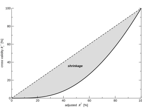
approximated analytically for the first time byLorenz(1956). A refined estimate can be described as follows: Let ˜R2 denote the squared mulitple correlation of a model with

p predictors estimated from a sample of N years, adjusted for p (cf. Seber and Lee,

2003). From that, an unbiased estimate of the squared correlation to be expected from

10

a prediction is calculated as (Nicholson,1960;Cattin,1980):

ˆ

R_c2 = (N − 1) ˜R 4

+ ˜R2

(N − p) ˜R2_{+ p} (4)

This estimate of Rc2, also called the cross validity, thus describes the shrinkage in

skill that is to be expected for predictions of a model estimated fromN years and p

predictors, having an adjusted calibration skill of ˜R2. The dependence of ˆRc2 on ˜R

2 is

15

shown in Fig.1 for the P and T setting with N=127 and p=22. Even with very large multiple correlations the cross-validity remains quite moderate, so that, for example, to achieve ˆRc2=50% one already needs ˜R

2

=80%. Conversely, a score of ˜R2=36%, as for regressing NHT from the full instrumental period, dramatically shrinks to a cross validity of only 6%.

20

Equation (4) applies to models estimated by ordinary least squares and thus to all reconstructions (“predictions”) that are based on some form of multiple regression. It should illustrate the order of magnitude that is to be expected from shrinking, given a ratio of predictors and sample size that is typical for millennial climate reconstructions. Estimates based on multi-crossvalidation shall be provided in §5.

(10)

CPD

EGU 3 The trivial NHT predictor

Having studied the close relation betweenRE and CE via the calibration mean bias, α, let us turn our attention now to the possible causes of such bias, using a very

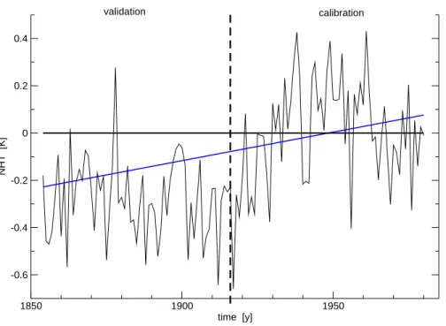
basic example. Figure 2 shows the average NHT as estimated from the set of 219 temperature grid points, T . There is an obvious imbalance between the early and the

5

late half of the period: while colder, even cooling conditions prevail in the early portion, much warmer conditions, initiated by a strong positive trend between 1920 and 1940, dominate the second half. Along with NHT, the linear model is plotted that results from regressing the late portion (1917–1980) against a very simple predictor: the series of calendar years. I will call this the trivial model or trivial predictor. This is in effect

10

nothing more than fitting a linear trend to that portion. And as a positive trend, the trivial model predicts colder conditions for the past earlier portion. While this does not seem to be an overwhelming performance, the model attains for that part (1854–1916) a verificationRE score of 56%! Recalling that RE measures the relative improvement

to the climatology forecast, ¯x_c, indicated by the zero line, the trivial model outperformes

15

that forecast easily by simply predicting colder conditions.

On the other hand, the trivial prediction attains a CE of –70%. According to Eq.

(3), this large discrepancy is caused by the enormeous bias in the calibration mean of

α=1.7 standard deviations (recall that α=1.2 from the last section is based on a 1902–

1980 calibration period). At this point it is important to understand what – besides the

20

presence of the overall trend – leads to that bias. The trend is obviously only effective because of the clean temporal separation of calibration and validation sets. Large values of α, and thus high RE scores, are obtained because of a) a positive trend

in the late calibration andb) negative anomalies in the early validation. In general, it

needs a calibration trend of the same sign as the mean difference between late and

25

the early portion.

To clarify the interplay between trend and the degree of temporal separation the following Monte Carlo exercise is performed. Starting from the original partition with

(11)

CPD

EGU the 1917–1980 (1854–1916) late calibration (early validation) period, single calibration

and validation years are iteratively swapped, the latter being picked randomly, and a regression model is calibrated. After a certain amount of swappings, here 100, the ini-tial separation is lost and calibration and validation years are equally distributed. Each of the generated configurations is now once more “mirrored” by exchanging

calibra-5

tion and validation sets. For each step, the individual degree of separation can be measured, for example, by the relative difference

degree of separation = T¯c− ¯Tv ¯

Tlate− ¯Tearly

(5)

where ¯T indicates the mean of the respective calendar years (with subscripts c and v

indicating calibration and validation, respectively). In each step the verification scores

10

RE and CE of the corresponding model are calculated, relating it to the degree of

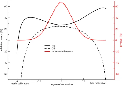
separation. Each single relation is, however, bound to be noisy due to the random selections of calendar years. The above is therefore repeated 500 times to study the average behavior, as shown in Fig.3. It shows a smooth dependence of the average

RE and CE values on the degree of temporal separation. Both scores show opposite

15

behavior, with RE preferring positive and CE negative values. RE values rise from

about 30% for the full mixture to almost 60% for the full separation of the late calibration, while the early calibration shows much lower scores due to the missing, or negative, trend there. CE is more symmetric about the full mixture. There, CE nearly equals RE , while it strongly decreases to about –50% at both ends of the full separation. It is

20

thus found that a trend creates enormeousRE scores, but at least half of it is due to

the particular selection of calibration and validation sets.

The statistics of each single calibration set is now, with varying degree, representa-tive of the full set (population). As a simple measure of that representarepresenta-tiveness one can, for example, test the hypothesis that the NHT values from the calibration and

25

those of the full set are equally distributed, using the Mann-Whitney (ranksum) test, and take the resulting p-value. Accordingly averaged over the 500 realizations one

(12)

CPD

EGU finds, not surprisingly, a strong dependence of that index on the degree of separation

(see Fig.3). It is symmetric about zero separation, i.e. full mixture, with a maximum attained there and calibration sets that are representative. At both ends, under full sep-aration, the values are practically zero and the calibration sets not representative. It is at these minima where both scores, RE and CE , happen to show the most extreme

5

values.

Note that this representativeness is closely related to the missing-at-random (MAR) criterion that is important for the imputation of missing data and algorithms such as EM and RegEM (see below; cf.Rubin,1976;Little and Rubin,1987). It is also relevant for the extrapolation argument given byB ¨urger and Cubasch(2005).

10

One could have used other predictors, such as, for example, the number of reporting stations for the temperature grid points (which scores 35%RE for the late calibration).

They will give similar results as long as the predictor contains a trend. In view of the intended time span – the full millennium – however, such simple, trend-based predictors are obviously not useful as they would just extrapolate the trend backwards into the

15

millennium and produce unrealistic cooling. Hence, at least in this simple case not much useful information is to be expected from theRE scores.

I will now turn to “real” predictors, that is, proxy information made up of tree-rings, corals, ice cores, etc., and the more sophisticated empirical models that make use of them.

20

4 Reconstruction flavors

Several statistical methods exist or have extra been developed to derive millennial NHT from proxy information. They are distinguished by using or not using a number of independent options in the derivation of the final temperature from the proxies. These options mainly pertain to the specific choice of the preprocessing, the statistical model,

25

and the postprocessing.

(13)

func-CPD

EGU tion and those which employ direct infilling of the missing data. In the first approach,

the heterogeneous proxy information is transformed to a temperature series by means of a transfer function that is estimated from the period of overlapping data. In the sec-ond approach, data are successively infilled to give a completed dataset that is most consistent (see below) with the original data. The transfer function approach uses

ei-5

ther some a priori weighting of the proxies, based on, e.g., areal representation, or a weighting directly fitted from the data, that is, multiple regression. To reduce the num-ber of weights in favor of significance, several filtering techniques can be applied, such as averaging or EOF truncation on both the predictor (Briffa et al.,1988,1992) and the predictand side (MBH98;Evans et al.,2002;Luterbacher et al.,2002).

10

4.1 Preprocessing (PRE) Besides using

1) NHT directly as a target, that is, calibrating the empirical model with the NH mean

of the T series, so that no spatial detail is modeled at all, intermediate targets can be defined, as follows:

15

2) PC truncation. Here a model is calibrated from the dominant principal components

(PCs) of T , and a hemispheric mean is calculated from their reconstruction. This is applied by MBH98, who have used a single PC. To be compatible with that study I also used only one PC (explaining about 20%–30% depending on the calibration set).

3) full set. The third possibility, applied byMann and Rutherford(2002);Rutherford

20

et al. (2003,2005);Mann et al.(2005), does not apply any reduction at all to the target quantity, treating the entire set of temperature grid points (more than 1000 in those studies) as missing. In our emulation, the full set T of 219 temperature grid points is set to missing. From the reconstructed series the NH mean is calculated.

(14)

CPD

EGU 4.2 Statistical method (METH)

The reconstruction of temperatures from proxies can be viewed in the broader context of infilling missing values. The infilling is done by using either a transfer function be-tween knowns and unknowns that is fitted in the calibration (1–4 below), or in a direct way using iterative techniques (5, 6):

5

1) Classical (forward) regression. Between the known P and unknown T quantities,

a linear relation R is assumed, as follows:

T = RP + ε, (6)

whereε represents unresolved noise. The matrix R = Σ−1_P_{ΣPT, with Σ}xy denoting the

cross covariance matrix between x and y (taking Σx = Σxx), is determined by least

10

squares (LS) regression, with T assumed to be noisy.

2) Inverse (backward) regression. This method is applied by MBH98. It also uses

a linear model as in 1), but now P is assumed noisy, leading to the LS estimate RI = Σ+_TPΣT, (“+” denoting pseudo inverse).

3) Truncated total least squares (TTLS). This form of regression, in combining 1)

15

and 2), assumes errors in both quantities P and T (cf.Golub and Loan,1996). The 10 major singular values were retained.

4) Ridge regression. As 1) , but with an extra offset given to the diagonal elements

of the (possibly ill-conditioned) matrix ΣP used as regularization parameters (Hoerl, 1962).

20

5) EM. Unlike using a fixed transfer function defined from a calibration set, there are

methods that exploit all available information when infilling data, including those from a validation predictor set. A very popular method uses the Expectation-Maximization (EM) algorithm, which provides maximum-likelihood estimates of statistical parameters in the presence of missing data (Dempster et al.,1977). EM is applied using the more

25

specialized regularized EM algorithm, RegEM (see below), with a vanishing regular-ization parameter.

(15)

CPD

EGU

6) RegEM. RegEM has been invented to utilize the EM algorithm for the estimation

of mean and covariance in ill-posed problems with fewer cases than unknowns (cf. Schneider,2001). It was intended for, and first applied to, the interpolation/completion of large climatic data sets, such as gridded temperature observations, with a limited number of missing values (3% inSchneider,2001). The technique was then extended

5

to proxy-based climate reconstructions (with a rate of missing values easily approach-ing 50%) and seen as a successor of the MBH98 method (Mann and Rutherford,2002; Rutherford et al.,2003,2005;Mann et al.,2005). Note, however, that millennial appli-cations utilize rather few proxies, so that the infilling problem is no longer ill-posed and the much simpler EM could have been used. Moreover, the reported millennial

verifica-10

tionRE of RegEM is less than that of the original MBH98 (cf.Rutherford et al.,2005). The performance of EM and RegEM are here compared for the first time. Details on RegEM are given in the Appendix.

4.3 Postprocessing (POST)

In applications (e.g. verifications) the output of the statistical model is either taken 1) as

15

is or 2) rescaled to match the calibration variance (cf.Esper et al.,2005;B ¨urger et al., 2006). Note that this operation increases the expected model error.

As all of PRE, METH, and POST represent independent groups of options, they can be combined to form a possible reconstruction “flavor” (cf. B ¨urger et al., 2006). As a reference, each such flavor receives a code ϕ in the form of a triple from the set

20

{1,2,3}×{1,2,3,4,5,6}×{1,2}, indicating which options were selected from the 3 groups above. This defines a set of 3×6×2=36 flavors. For example, the MBH98 method corresponds to flavorϕ=222 andRutherford et al.(2005) toϕ=161. Table1illustrates the various settings.

(16)

CPD

EGU 5 Multi-crossvalidation of NHT reconstructions

I consider 300 random partitionsπ of the set I= {1854, ..., 1980} of calendar years,

I = Cπ ∪ Vπ, (7)

into calibration and validation sets C_πand V_π, where both sets are roughly of equal size (|Cπ|=64 and |Vπ|=63). For any of the 36 flavors, ϕ, it is now possible to calibrate an

5

empirical model, with corresponding scoresRE_ϕ(π) and CE_ϕ(π). RE_ϕ(π) and CE_ϕ(π)

thus appear as realizations of random variablesREϕandCEϕ, with corresponding

dis-tributions. Along with the 300 random partitions I also consider the two complementary partitions with full temporal separation.

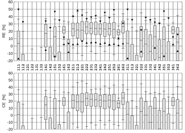
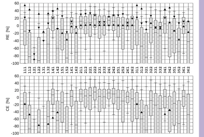
The distributions ofREϕ and CEϕ are depicted in Fig.4as a boxplot. For most

fla-10

vors the distributions show a remarkable spread, with minimum and maximum (low and high 10%-quantiles) easily departed by more than 50% (20%) of skill. Moreover, be-tween the flavors the distributions are quite different. For example, the flavors ϕ=161 andϕ=162 are merely distinguished by the use of rescaling. Their performance,

how-ever, is grossly different. This applies likewise to the flavors ϕ=141/2 and ϕ=151/2,

15

so that at least in these cases skill is strongly degraded by rescaling (note, however,

ϕ=261/2). While there is so much spread in skill within and between the flavors the

distributions themselves are quite similar for both scoresRE_ϕ andCE_ϕ. This indicates that, in fact, most calibration/validation partitions are temporally well mixed andRE_ϕ

andCEϕ measure the same thing (see §3).

20

The skill varies, but it varies on rather low levels. The 90% quantile hardly exceeds the 30% mark, and the highest median isRE_ϕ=26.5% and CEϕ=24.6% for ϕ=262.

Generally, flavors of the form 2xx, i.e. those predicting PC1 of NHT, perform much bet-ter, with almost all medians above 20%. The other flavors are much more variable, partly caused by the degradation from rescaling mentioned above. An exception are

25

the flavors of the form x61 which show remarkably little variance (albeit only moderate scores). This is understandable insofar as RegEM, unlike the other flavors, depends on

(17)

CPD

EGU the particular calibration set only in terms of the predictand (utilizing the full

instrumen-tal period for the predictors). This would also apply to the EM flavors (x51), but they are probably more susceptible to overfitting. Note that the flavorϕ=311, which has shortly

been touched in §2 to exemplify shrinking, scores very little, withRE and CE values

below 5%. This is about the same order of magnitude as the estimate obtained from

5

Eq. (4).

The mindful reader has noticed that some flavors, such asϕ=111 and ϕ=311, have

identical distributions. In fact, for direct regression, with a linear dependence of the estimated model on the predictand, cf. §4.2, they are equivalent with respect to NHT and thus redundant. (Note that the RegEM flavorsϕ=161 and ϕ=361 are similar as

10

well.)

The triangles in the figure represent the two calibrations with full temporal separation, i.e. the periods 1917–1980 (upper triangle) and 1854–1916 (lower triangle). They are more comparable to estimates of previous studies and obviously assume the role of outliers, in a positive sense for RE and in a negative one for CE . While several RE

15

values approach 50% theCE values are negative throughout. Models with trended and

fully separated calibration sets are thus rewarded with highRE scores but penalized

with lowCE scores.

Based on such levels of performance it is difficult to declare one specific flavor as being the “winner” and being superior to others. Just from the numbers, the flavor

20

ϕ=262 gives the best RE perfomance (see above). It predicts PC1 using RegEM and

rescaling. But it is only marginally better than, e.g., the simpler variant 211 (simple forward regression, with median 23.4%). Note that the flavor 161 was promoted by Mann et al. (2005) and earlier to replace the original MBH98 flavor 222. From the current analysis, this cannot be justified (RE median of 21.8% compared to 25.9%).

25

This is somewhat in agreement withRutherford et al. (2005) who report a millennial

RE of 40% (46% for the “hybrid” case), as compared to the 51% of MBH98. Moreover,

for the late calibration the 161 flavor is particularly bad (RE_ϕ=11.9%); it improves, nonetheless, when calibrating with the “classical” calibration period 1902–1980 (28%).

(18)

CPD

EGU 6 Significance

There is an ongoing confusion regarding the notion of significance of the estimated reconstruction skill. For the same model (the one used by MBH98, here the emulated flavor 222), MBH98 (resp.Huybers,2005) andMcIntyre and McKitrick(2005b) report a 99% significance level forRE as different as 0% and 54%! Hence, with a reported RE

5

of 51% the model is strongly significant in the first interpretation and practically useless, i.e. indistinguishable from noise, in the latter. And what might be even more intriguing: The trivial model of §3 with an RE score of 56% turns out to be significantly skillful

under both interpretations. Obviously, the notion of “being significant”, or of being a “nonsense predictor”, deserves a closer look.

10

A major difference in the two approaches is the allowance for nonsense regressors for the significance estimation, because only that yields higher scores. Now even in the well-mixed, representative case the trivial predictor scored about 20% in bothRE and CE , which would still be significantly skillfull under a significane level of 0%. To avoid

this, nonsense regressors must therefore be allowed. On the other hand we have seen

15

how the temporal separation produces non-representative samples, and createsRE

“outliers” of up to 60%. The proposed significance level ofRE =54%, which is based

on these outliers, is thus equally inflated and must be replaced by something more representative.

A crucial question is: What kind of nonsense predictors should be allowed? – To

20

derive a statistically sound significance level requires a null distribution of nonsense reconstructions. Now one can think of all sorts of funny predictors, things like calen-dar years, Indias GDP, the car sales in the U.S., or all together, etc., but that will not make up what mathematically is called a measurable set (to which probabilities can be assigned). Hence, a universal distribution of nonsense predictors does not exist.

25

– A more managable type of nonsense predictors are stochastic processes generated from white noise, such as AR, ARMA, ARFIMA, ..., (cf. Brockwell and Davis, 1998). Once we fix the number of regressors, the type of model, say ARMA(p,q), and the set

(19)

CPD

EGU of parameters, a unique null distribution of scores can be obtained from Monte Carlo

experiments. From these, a significance level can be estimated and compared to the original score of the reconstruction. The only problem is then that each of the specified stochastic types creates its own significance level.

It was perhaps this dilemma that originated the debate about the benchmarking of

5

RE , specifically, estimating the 99% level of significance, REcrit. In the literature, one finds the following approaches:

1. (MBH98) simple AR(1) process with specified memory:RE_crit= 0%;

2. (MM05) inverse regression of NHT on a red noise predictor, estimated from one of the 22 proxies (the dominant PC of North American tree ring network):REcrit = 10

59%;

3. (Huybers,2005) as2, with rescaling: REcrit = 36% using red noise version from accompanying matlab code (10 000 samples);

4. (McIntyre and McKitrick,2005b) as3, but with 21 additional (uncorrelated?) white noise predictors: REcrit= 54%.

15

One might now feel inclined to provide the “correct” or “optimum” way of repre-senting the proxies as a stochastic process. If I now add

5. as4, but with all noise predictors (not only PC1) estimated from the original prox-ies,

the series of benchmarking attempts from1to5would in fact slowly convergence to

20

what MBH98 and similar studies should be compared to. But so much is not required. One can and must only provide a realistic lower bound on the level of significance, may it come from whatever stochastic process. With regard to 5, a benchmark has not been estimated so far, and will not be estimated here. The lesson of §3 is that all benchmarks 1–4 are inflated by the temporal separation of calibration and validation

25

(20)

CPD

EGU For each of the 36 flavors I have therefore repeated the analysis of §5, with the

proxies being replaced by red noise series. Specifically, for each proxy a stochastic long-memory process is generated whose memory parameter,d , is estimated from the

proxy using log-periodogram regression (Geweke and Porter-Hudak,1983;Brockwell and Davis,1998). To obtain more robust estimates ofd I used here, like MM05, the full

5

proxy record from 1400 to 1980; the corresponding estimates varied betweend =−0.17

and d =0.85. Note that the log-periodogram estimation is slightly different from the

method suggested byHosking(1984) and applied by MM05. Neither method is perfect, as both rest on various approximations (cf.Bhansali and Kokoszka,2001) that provide little more than a rough guess of what the “true” long-memory parameter might be. But

10

again, such kind of truth is not required.

The noise generation was redone in each of the 300 iterations (to remove sampling effects). The result is shown in Fig. 5. Like in Fig. 4, RE and CE values are

sim-ilar. All scores are smaller compared to the corresponding proxy predictions, with a greater spread per flavor. They are nonetheless not neglegible. Analoguously to the

15

proxies, the scores are generally better for flavors of the form 2xx, with median levels varying about 10%. For each flavor, also included are the experiments with full tem-poral separation. Some of theRE scores exceed 50%, like the trivial predictor (54%

forϕ=311). As an example, Fig.6shows the distribution of the 300 predictions for the flavor _{ϕ=222, in terms of validation RE and in comparison to the proxy predictions.}

20

We clearly see different distributions, the nonsense predictions being more spread and generally shifted to smaller RE values, varying roughly about 20%. Note that this is

about the score of the trivial predictor for representative calibration sets, depicted in Fig.3. There are nonetheless outliers with very good scores (∼45%). These are possi-ble, as we saw, if the predictors are sufficiently persistent, and calibration and validation

25

sufficiently separated in the time domain.

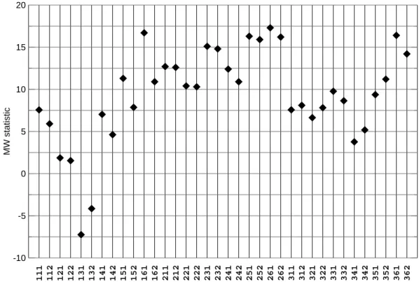
The degree to which the proxy predictions outperform their nonsense pendants is depicted in the last Fig.7; it shows for each flavor the respective Mann-Whitney test statistic. Except for the flavors_{ϕ=13x the values are well beyond the 99% level of the}

(21)

CPD

EGU standard normal null distribution of the test (obtained if both samples come from the

same population). The highest values are, like in Fig.4, attained by the 2xx flavors that are based on predictand EOF filtering. The x61 flavors, i.e. those using RegEM, are also large, which is possibly due to the overall reduction inRE spread for those flavors

(see above).

5

Now one thing is still unresolved: Why do the nonsense predictions have non-vanishing score even for the well mixed, representative samples? – A nonsense predic-tion has, by definipredic-tion, no skill. In an ideal world, which among other things has infinite samples and truely independent validation, it would yield a cross-validity ofR_c = 0 and thus, using Eq. (2),CE ≤0 (see §2); and RE would at best be artificially inflated via the

10

α bias, from Eq. (3). Positive scores of nonsense predictions are therefore an artefact of the limited sample of 127 cases/years. In fact, in the finite case, calibration and vali-dation sets are never fully independent; they become more and more dependent if the memory of the time series gets comparable to the series length. The most plausible explanation for the spurious skill is therefore: that the validity of a regression will be

15

partly inherited by the “independent” verification period and create skill there.

This argument applies equally to the proxy predictions. Therefore, about 10% of the 25% skill are likely caused by spurious skill due to memory effects.

7 Conclusions

The analysis poses three quesions:

20

1. How do we interpret the estimated levels of reconstruction skill? 2. How do we interpret the resulting spread in that skill?

3. How are possible answers to 1. and 2. affected by the significance analysis?

ad 1: It was found that realistic estimates of skill vary about 25%, equally for RE

and CE . The results were obtained using a well confined testbed of proxy and

(22)

CPD

EGU perature information through 127 instrumental years, with almost no gaps. The proxies

represent a standard set of what is available back to AD 1400. The set of tempera-ture grid points does not cover the entire globe, and its areal averages serve only as approximations to the full NHT average; but it is about the largest subset that is rig-orously verifiable. On this background, previous estimates of NHT reconstruction skill

5

in the range of RE =50% appear much too large. They are inflated by the use of a

non-representative calibration/validation setting in the presence of trended data.

ad 2: Crossvalidation of any type (single, double, multi) is a means to estimate

the distribution of unknowns (here: the reconstruction skill). As there is no a priori criterion to prefer a specific calibration set, all such sets receive equal weights before

10

and after the analysis (this is somewhat in conflict withRutherford et al. (2003) who seem to prefer one set because of its validation skill). The estimated distributions were quite similar forRE and CE , indicating that both scores actually measure the same

thing. The considerable spread of most distributions simply reflects our limited ability to estimate skill any better, based on a sample size of 127 cases/years, and on an

15

effective sample size that is even less, due to persistence.

ad 3: Reconstructions based on real proxies significantly outperform the chosen

class of nonsense predictions (based on stochastic long-memory processes). It is unknown whether they outperform any such class, as strong persistence, like in the trivial predictor, enhances scores. Most flavors, moreover, reveal a non-vanishing score

20

for the nonsense predictors, varying about 10% for many flavors. This was attributed to the degraded independence of the finite validation period by memory effects, allowing portions of the calibration information to drop into the validation. As this is equally true for the proxy predictions, a significant amount of the estimated verification skill is likely to be spurious, and further adjustments are necessary.

25

It is unknown how such an adjustment should be done numerically, producing a final overall verification skill that for the best flavors is somewhere between 15% and 25%, with large uncertainties. With respect to applications, that is, reconstructions, the main question is, however: Are these levels sufficient to decide the millennial NHT

(23)

contro-CPD

EGU versy? – 25%RE translates to an amplitude error of √100_{−RE∼ 85%. If one were}

to focus the controversy into the single question: Was there a hemispheric Medieval Warm Period and was it possibly warmer than recent decades? – that question cannot be decided based on current reconstructions alone, at least not in a verifiable sense.

Appendix A

5

RE , CE , and R_c

Suppose true (verification) and predicted values are given by x and ˆx, respectively.

Without loss of generality let us assumehxi=0 . There are now three forms of relative bias, the calibration mean bias,α = _√x¯c

hx2_i , and the two biases in mean,β= h ˆxi √ hx2_i , and 10 amplitude,γ= r h( ˆx−h ˆxi)2_i

hx2_i . Using these, we have

CE = 1 −h( ˆx − x) 2 i hx2_i = hx 2 i − h ˆx2i + 2h ˆxxi − hx2i hx2_i = 2h ˆxxi − h ˆx 2 i hx2_i = 2h( ˆx − h ˆxi)xi − h( ˆx − h ˆxi) 2

i + 2hxih ˆxi − 2h ˆxi2+h ˆxi2 hx2_i 15 = 2h( ˆx − h ˆxi)xi − h( ˆx − h ˆxi) 2 i hx2_i − h ˆxi2 hx2_i

(24)

CPD

Printer-friendly Version Interactive Discussion EGU = 2_qh( ˆx − h ˆxi)xi h( ˆx − h ˆxi)2ihx2_i q

h( ˆx − h ˆxi)2i/hx2_{i − h( ˆx − h ˆxi)}2_i/hx2

i − h ˆxi2/hx2i

= γ(2Rc− γ) − β2 (A1)

withRcdenoting the correlation between predicted and true values. Now we have

RE = 1 − h( ˆx − x) 2 i h(x − xc)2i =hx 2 i − 2hxxci + hx 2 ci − h ˆx 2 i + 2h ˆxxi − hx2i hx2_{i − 2hxx} ci + hxc2i 5 =2h ˆxxi − h ˆx 2 i + xc2 hx2_{i + hx}2 ci =CEhx 2 i + x2c hx2_{i + hx}2 ci =CE + α 2 1 + α2 (A2)

Note that the 4th line of Eq. (A2) is an immediate consequence of the 3rd line of Eq. (A1).

10

Appendix B

RegEM configuration

To control the iteration, RegEM has a number of configuration switches that can be adjusted. The following settings gave satisfactory convergence results for most of the

(25)

CPD

EGU experiments. I used: multiple ridge regression as a regression procedure;

regular-ization parameter determined from general cross validation (GCV); minimum relative variance of residuals: 5e-2; stagnation tolerance: 3e-5; maximum number of iterations: 50; inflation factor: 1.0; minimum fraction of retained variance: 0.95. This latter setting is borrowed fromRutherford et al.(2003) who argue that the GCV regularization

esti-5

mate is too crude in the presence of too many unknowns. This was true here as well. In fact, using the GCV estimate for the flavorsϕ=1xx resulted in RegEM reconstructions

that were hardly distinguishable from the calibration mean.

Acknowledgements. I enjoyed lively discussions with U. Cubasch, F. Nieh ¨orster and F. Kaspar.

This work was partly supported by the EU project SOAP. 10

References

Aldrich, J.: Correlations Genuine and Spurious in Pearson and Yule, Discussion Paper Se-ries In Economics And Econometrics 9502, Economics Division, School of Social Sciences, University of Southampton, available at:http://ideas.repec.org/p/stn/sotoec/9502.html, 1995.

253

15

Bhansali, R. J. and Kokoszka, P. S.: Estimation of the long memory parameter: a review of recent developments and an extension, in: Selected proceedings of the symposium on in-ference for stochastic processes. IMS Lecture notes and monograph series, edited by: Ba-sawa., I., Heyde, C. C., and Taylor, R., 125–150, Institute of Mathematical Statistics, Ohio, USA, 2001. 267

20

Briffa, K. R.: Annual climate variability in the holocene: intepreting the message of ancient trees, Quat. Sci. Rev., 19, 87–105, 2000. 251

Briffa, K. R., Jones, P. D., Pilcher, J. R., and Hughes, M. K.: Reconstructing Summer Temper-atures in Northern Fennoscandinavia Back to A.D.1700 Using Tree Ring Data from Scots Pine, Arctic and Alpine Research, 385–94, 1988. 252,254,255,260

25

Briffa, K. R., Bartholin, T. S., Eckstein, D., Jones, P. D., Karlen, W., Schweingruber, F. H., and Zetterberg, P.: A 1,400-year tree-ring record of summer temperatures in fennoscandia, Nature, 346, pp. 434–439, 1990. 252

(26)

CPD

EGU

Briffa, K. R., Jones, P. D., and Schweingruber, F. H.: Tree-ring density reconstructions of sum-mer temperature patterns across western north asum-merica since 1600, J. Climate, 5, 735–754, 1992. 252,254,260

Briffa, K. R., Osborn, T. J., Schweingruber, F. H., Harris, I. C., Jones, P. D., Shiyatov, S. G., and Vaganov, E. A.: Low-frequency temperature variations from a northern tree ring density 5

network, J. Geophys. Res., 106(D3), 2929–2941, 2001. 251,254

Brockwell, P. J. and Davis, R. A.: Time series: theory and methods, 2nd edition, Springer Series in Statistics, 1998. 265,267

B ¨urger, G. and Cubasch, U.: Are multiproxy climate reconstructions robust?, Geophys. Res. Lett., L23711, doi:10.1029/2005GL0241 550, 2005. 251,259

10

B ¨urger, G., Fast, I., and Cubasch, U.: Climate reconstruction by regression – 32 variations on a theme, Tellus A, 227–35, 2006. 251,252,262

Cattin, P.: Estimation of the predictive power of a regression model, J. Appl. Psychol., 65(4), 407–414, 1980. 252,256

Cook, E. R., Briffa, K. R., and Jones, P. D.: Spatial regression methods in dendroclimatology: 15

a review and comparison of two techniques, Int. J. Clim., 379–402, 1994. 254

Cook, E. R., Buckley, B. M., D’Arrigo, R. D., and Peterson, M. J.: Warm-season temperatures since 1600 bc reconstructed from tasmanian tree rings and their relationship to large-scale sea surface temperature anomalies., Clim. Dyn., 16, 79–91, 2000. 252

Cooley, W. W. and Lohnes, P. R.: Multivariate data analysis, New York: Wiley, 1971.251

20

Crowley, T. J. and Lowery, T. S.: How warm was the medieval warm period?, Ambio, 29, 54, 2000. 251,254

Dempster, A., Laird, N., and Rubin, D.: Maximum likelihood estimation from incomplete data via the EM algorithm, J. Royal Statist. Soc., B, 39, 1–38, 1977.261

Efron, B.: Bootstrap methods: another look at the jackknife, Annals of Statistics, 17, 1–26, 25

1979. 252

Efron, B. and Gong, G.: A Leisurely Look at the Bootstrap, the Jackknife, and Cross-Validation, American Statistician, 36–48, 1983. 252

Esper, J., Cook, E. R., and Schweingruber, F. H.: Low frequency signals in long tree-ring chronologies for reconstructing past temperature variability, Science, 295, 2250–2253, 2002. 30

251,254

Esper, J., Frank, D. C., Wilson, R. J. S., and Briffa, K. R.: Effect of scaling and regression on reconstructed temperature amplitude for the past millennium, Geophysical Research Letters,

(27)

CPD

EGU

Volume 32, Issue 7, 32(7), L07711, 2005.262

Evans, M. N., Kaplan, A., and Cane, M. A.: Pacific sea surface temperature field reconstruction from coral delta o-18 data using reduced space objective analysis, Paleoceanography, 17, 1007, 2002. 260

Fritts, H. C.: Tree rings and climate, Academic Press, 1976.254

5

Fritts, H. C. and Guiot, J.: Methods of calibration, verification, and reconstruction, in: Methods Of Dendrochronology. Applications In The Environmental Sciences, edited by: Cook, E. R. and Kairiukstis, L. A., 163–217, Kluwer Academic Publishers, 1990. 252

Geweke, J. and Porter-Hudak, S.: The estimation and application of long-memory time series models, J. Time Series Analysis, 4, 221–238, 1983. 267

10

Golub, G. H. and Loan, C. F. V.: Matrix computations (3rd ed.), Johns Hopkins University Press, Baltimore MD USA, 1996. 261

Guiot, J., Nicault, A., Rathgeber, C., Edouard, J. L., Guibal, E., Pichard, G., and Till, C.: Last-millennium summer-temperature variations in western europe based on proxy data, Holocene, 15, 500, 2005.252

15

Hoerl, A. E.: Application of ridge analysis to regression problems, Chem. Eng. Prog., 58, 54– 59, 1962. 261

Hosking, J.: Modeling persistence in hydrological time series using fractional differencing, Wa-ter Resour. Res., 20(12), 1898–1908, 1984. 267

Huybers, P.: Comment on ''Hockey sticks, principal components, and spurious significance'', 20

Geophys. Res. Lett., L20705, doi:10.1029/2005GL023395, 2005.251,265,266

IPCC: Climate change 2001: the scientific basis. contribution of working group I to the third assessment report of the intergovernmental panel on climate change, Cambridge University Press, Cambridge, 2001. 251

Jones, P. D., Briffa, K. R., Barnett, T. P., and Tett, S. F. B.: High-Resolution Palaeoclimatic 25

Records for the Last Millennium: Interpretation, Integration and Comparison with General Circulation Model Control-Run Temperatures, Holocene, 8, 455–71, 1998.250,254

Krus, D. J. and Fuller, E. A.: Computer assisted multicrossvalidation in regression analysis, Educational and Psychological Measurement, 42, 187–193, 1982. 252

Little, R. J. A. and Rubin, D. B.: Statistical analysis with missing data, Wiley, 1987.259

30

Lorenz, E. N.: Empirical orthogonal functions and statistical weather prediction, Sci. Rept. No. 1, Dept. of Met., M. I. T., p. 49pp, 1956. 254,256

(28)

CPD

EGU

Schmutz, C., and Wanner, H.: Reconstruction of sea level pressure fields over the east-ern north atlantic and europe back to 1500, CLIMATE DYNAMICS, 18, 545–561, 2002.252,

260

Mann, M. E. and Rutherford, S.: Climate reconstruction using 'Pseudoproxies', Geophys. Res. Lett., p. 139, 2002. 260,262

5

Mann, M. E., Bradley, R. S., and Hughes, M. K.: Global-scale temperature patterns and climate forcing over the past six centuries, Nature, 779–87, 1998. 250

Mann, M. E., Bradley, R. S., and Hughes, M. K.: Northern hemisphere temperatures during the past millennium: inferences, uncertainties, and limitations, Geophys. Res. Lett., 759–762, 1999. 250,252

10

Mann, M. E., Rutherford, S., Wahl, E., and Ammann, C.: Testing the Fidelity of Methods Used in Proxy-Based Reconstructions of Past Climate, J. Climate, 4097–107, 2005.251,255,260,

262,264

McIntyre, S. and McKitrick, R.: Corrections to the Mann et al. (1998) proxy data base and northern hemispheric average temperature series, Energy Environ., 14(6), 751–771, 2003. 15

251

McIntyre, S. and McKitrick, R.: Hockey sticks, principal components and spurious significance, Geoph. Res. Let., 32, L03710, doi:10.1029/2004GL021750, 2005a. 251

McIntyre, S. and McKitrick, R.: Reply to comment by huybers on ''hockey sticks,

principal components, and spurious significance'', Geophys. Res. Lett., 32, L20713, 20

doi:10.1029/2005GL023586, 2005b. 251,265,266

Moberg, A., Sonechkin, D. M., Holmgren, K., Datsenko, N. M., and Karlen, W.: Highly variable northern hemisphere temperatures reconstructed from low- and high-resolution proxy data, Nature, 433, 617, 2005.251

Nash, J. E. and Sutcliffe, J. V.: River flow forecasting through conceptual models - Part I - A 25

discussion of principles, J. Hydrol., (10), 282–90, 1970. 254

Nicholson, G. E.: Prediction in future samples, in: Contributions to Probability and Statistics, edited by: Olkin, I., 322–330, 1960. 256

Overpeck, J., Hughen, K., Hardy, D., Bradley, R., Case, R., Douglas, M., Finney, B., Gajewski, K., Jacoby, G., Jennings, A., Lamoureux, S., Lasca, A., MacDonald, G., Moore, J., Retelle, 30

M., Smith, S., Wolfe, A., and Zielinski, G.: Arctic Environmental Change of the Last Four Centuries, Science, 278, 1251–1256, 1997. 250,254

(29)

CPD

EGU

Correlation Which May Arise When Indices Are Used in the Measurement of Organs, Proc. R. Soc., 60, 489–498, 1897. 253

Raju, N. S., Bilgic, R., Edwards, J. E., and Fleer, P. F.: Methodology review: estimation of population validity and cross-validity, and the use of equal weights in prediction, J Appl. Psychol. Measurement, 21(4), 291–305, 1997. 252

5

Rubin, D. B.: Inference and missing data, Biometrika, 63, 581–592, 1976.259

Rutherford, S., Mann, M. E., Delworth, T. L., and Stouffer, R. J.: Climate field reconstruction under stationary and nonstationary forcing, J. Climate, 16, 462–479, 2003. 252,260,262,

269,272

Rutherford, S., Mann, M. E., Osborn, T. J., Bradley, R. S., Briffa, K. R., Hughes, M. K., and 10

Jones, P. D.: Northern Hemisphere Surface Temperature Reconstructions: Sensitivity to Methodology, Predictor Network, Target Season and Target Domain, J. Climate, 2308–29, 2005. 251,252,254,255,260,262,264

Schneider, T.: Analysis of incomplete climate data: estimation of mean values and covariance matrices and imputation of missing values, J. Climate, 14, 853–871, 2001. 262

15

von Storch, H., Zorita, E., Jones, J. M., Dmitriev, Y., and Tett, S. F. B.: Reconstructing Past Climate from Noisy Data, Science, 679–82, 2004. 251

Wahl, E. R. and Ammann, C. M.: Robustness of the Mann, Bradley, Hughes reconstruction of Northern hemisphere surface temperatures: Examination of criticisms based on the nature and processing of proxy climate evidence, Climatic Change, in press, 2007.251,255

20

Wahl, E. R., Ritson, D. M., and Ammann, C. M.: Comment on ”Reconstructing past climate from noisy data”, Science, 312, p. 529b, http://www.sciencemag.org/cgi/content/abstract/

312/5773/529b, doi:10.1126/science.1120866, 2006. 251,252

Wilks, D. S.: Statistical methods in the atmospheric sciences. an introduction, Academic Press, San Diego, 1995. 254

25

Yule, G. U.: Why do we sometimes get nonsense-correlations between time-series? – A study in sampling and the nature of time-series, J. Roy. Stat. Soc., 1–29, 1926.253

(30)

CPD

EGU

Table 1. Table of the 3×6×2=36 reconstruction flavors.

PRE METH POST

219 grid points forward regression no rescaling

1 EOF backward regression rescaling

1 global average TTLS

ridge regression EM RegEM

(31)

CPD

Printer-friendly Version Interactive Discussion EGU 0 20 40 60 80 100 adjusted R2 [%] 0 20 40 60 80 100 cross validity Rc 2 [%] shrinkage

(32)

CPD

Printer-friendly Version Interactive Discussion EGU 1850 1900 1950 time [y] -0.6 -0.4 -0.2 0 0.2 0.4 NHT [K] validation calibration

Fig. 2. NHT observed (thin black line) and predicted from the series of calendar years (blue

line). The model is calibrated in the late portion (1917–1980) and validated in the early portion (1854–1916), yielding a RE score of 56%. Also depicted is the climatology forecast of the

(33)

CPD

Printer-friendly Version Interactive Discussion EGU -1 -0.5 0 0.5 1 degree of separation -60 -40 -20 0 20 40 60 validation score [%] -60 -40 -20 0 20 40 60 p-value [%] RE CE representativeness

early calibration late calibration

Fig. 3. The dependence of the validation scoresRE and CE on the degree of temporal

sep-aration for the simple NHT predictor (see text). For the full sepsep-aration with a late (1917–1980) calibration and early (1854–1916) validationRE (solid black) approaches 60%, while the fully

mixed case attains only about 30%RE ; towards early calibration RE rises again to 40% but

then sharply drops to negative values.CE (dashed black) shows somewhat opposite behavior,

with strongly negative values for the full separation and values similar toRE in the mixed case.

Also shown is an index (see text) of the representativeness the corresponding calibration sets (red).

(34)

CPD

Printer-friendly Version Interactive Discussion EGU 111 112 121 122 131 132 141 142 151 152 161 162 211 212 221 222 231 232 241 242 251 252 261 262 311 312 321 322 331 332 341 342 351 352 361 362 -20 -10 0 10 20 30 40 50 60 RE [%] -20 -10 0 10 20 30 40 50 60 CE [%]

Fig. 4. Boxplot of the distribution of RE and CE for each of the 36 flavors, based on 300

resamplings of the calibration/verification period. Each box indicates the 10%, 50%, and 90% quantile, and the whiskers the minimum and maximum, of the distribution. Also shown are the scores obtained from the full separation into early (upward triangle) and late (downward triangle) calibration. For readability, some flavors/experiments are not shown (too negative).