Spatially explicit avalanche risk assessment linking Bayesian networks to a GIS

(1)

HAL Id: hal-00299378

https://hal.archives-ouvertes.fr/hal-00299378

Submitted on 26 Oct 2006

HAL is a multi-disciplinary open access

archive for the deposit and dissemination of

sci-entific research documents, whether they are

pub-lished or not. The documents may come from

teaching and research institutions in France or

abroad, or from public or private research centers.

L’archive ouverte pluridisciplinaire HAL, est

destinée au dépôt et à la diffusion de documents

scientifiques de niveau recherche, publiés ou non,

émanant des établissements d’enseignement et de

recherche français ou étrangers, des laboratoires

publics ou privés.

Spatially explicit avalanche risk assessment linking

Bayesian networks to a GIS

A. Grêt-Regamey, D. Straub

To cite this version:

A. Grêt-Regamey, D. Straub. Spatially explicit avalanche risk assessment linking Bayesian networks to

a GIS. Natural Hazards and Earth System Science, Copernicus Publications on behalf of the European

Geosciences Union, 2006, 6 (6), pp.911-926. �hal-00299378�

(2)

Nat. Hazards Earth Syst. Sci., 6, 911–926, 2006 www.nat-hazards-earth-syst-sci.net/6/911/2006/ © Author(s) 2006. This work is licensed under a Creative Commons License.

Natural Hazards

and Earth

System Sciences

Spatially explicit avalanche risk assessment linking Bayesian

networks to a GIS

A. Grˆet-Regamey1,2and D. Straub3

1_{WSL Swiss Federal Institute for Snow and Avalanche Research, Research Unit Ecosystem Boudaries, 7260 Davos,} Switzerland

2_{Eidgenössiche Technische Hochschule Zürich (ETHZ), ETH Hönggerberg, LEP, IRL: HIL H32.1, 8093 Zürich, Switzerland} 3_{Department of Civil and Environmental Engineering, University of California, Berkeley, CA 94720-1710, USA}

Received: 31 May 2006 – Revised: 16 October 2006 – Accepted: 22 October 2006 – Published: 26 October 2006

Abstract. Avalanche disasters are associated with significant

monetary losses. It is thus crucial that avalanche risk assess-ments are based on a consistent and proper assessment of the uncertainties involved in the modelling of the avalanche run-out zones and the estimations of the damage potential. We link a Bayesian network (BN) to a Geographic Information System (GIS) for avalanche risk assessment in order to facil-itate the explicit modelling of all relevant parameters, their causal relations and the involved uncertainties in a spatially explicit manner. The suggested procedure is illustrated for a case study area (Davos, Switzerland) located in the Swiss Alps. We discuss the potential of such a model by comparing the risks estimated using the probabilistic framework to those obtained by a traditional risk assessment procedure. The pre-sented model may serve as a basis for developing a consistent and unified risk assessment approach.

1 Introduction

Economical damages from natural hazards are on the rise (MunicheRe, 2006). In order to deal with the increasing costs associated with the damages to buildings, structures, and fatalities, decision-makers need suitable methods to es-timate the risks. Especially in mountainous areas such as the Swiss Alps, where snow avalanches (e.g. avalanche win-ter 1999) and floods (e.g. floods in 2000, 2002, 2005) have caused high costs in the last decade, there is a need for a con-sistent modelling of the risks. Risk analysis is recognized to be the best method for estimating the dangers from par-ticular natural hazards (e.g. Einstein, 1988; Cruden and Fell, 1997). Risk is defined as a function of the probabilities P(Ai)

Correspondence to: A. Grˆet-Regamey

(gret@nsl.ethz.ch)

of all potential events Ai and the expected consequences un-der these events C(Ai):

R =X

i

P (Ai) · C(Ai) (1)

C(Ai) can be understood as the product of the damage poten-tial and the corresponding vulnerability (e.g. Varnes, 1984; Morgan et al., 1992).

Estimations of risk using Eq. (1) are dependent on many variables subject to uncertainty. On the one hand, multiple authors have investigated the uncertainties related to the esti-mation of P (Ai)in recent years (e.g. Barbolini et al., 2003;

Ancey et al., 2003; Ancey, 2004). These studies, sited in the field of avalanche hazards, mainly concentrate on the sensi-tivity of avalanche run-out distances to model assumptions. Because land-use planning based on avalanche hazard maps relies on the calculated run-out distance, these model uncer-tainties can have large effects on the regional economical de-velopment. In Straub and Grˆet-Regamey (2006), we present a Bayesian probabilistic framework for modelling avalanche hazards, which serves as a basis for the risk assessment pre-sented in this paper. On the other hand, little attention was di-rected towards the assessment of the expected consequences

C(Ai), which is based on a combination of observational in-formation and expert opinion. As a consequence, studies quantifying uncertainties related to this part of the risk as-sessment are missing. However, failure to include these un-certainties in the risk calculation may lead to significant in-consistencies. Furthermore, explicitly addressing the uncer-tainties in the model facilitates future model improvements.

Bayesian Networks (BN) are known to facilitate the ex-plicit modelling of uncertainties in an integral probabilistic framework (Friis-Hansen, 2000; Faber et al., 2002). Based on acyclic graphs, BN provide a detailed evaluation of the joint influence of different input parameters on the risk. Al-lowing a traceable and concise representation of the causal relationships between the considered variables, this is also

(3)

912 A. Grˆet-Regamey and D. Straub: Avalanche risk assessment linking Bayesian network to a GIS highly useful for natural hazard risk assessment, which

in-volves various uncertain variables and requires communica-tion between interdisciplinary groups of specialists. To our knowledge, there are only few reported applications of BN in the field of natural hazards: Amendola et al. (2000) points out the use of BN to consider the chain of indirect damages caused by natural hazards. Antonucci et al. (2003) assess debris flow hazards using credal nets. Hincks et al. (2004) use dynamic BN to model volcanic hazards. Bayraktarli et al. (2005) suggest a generic framework for the assessment of natural hazard risks using BN, and Straub (2005) illustrates the potential of BN for rock-fall hazard ratings. All these studies, however, do not estimate risk in a spatially explicit manner, which is essential for land-use planning.

Geographic Information Systems (GIS) have the capacity to incorporate the complexities of spatial dimension within such analyses. A large number of GIS applications for natu-ral hazards have been developed, particularly during the past decade (e.g., Wadge et al., 1993; Carrara and Guzzetti, 1995; Chen et al., 2003; Bell and Glade, 2004). Until now, in spite of the recognized uncertainties in spatial models and data (Fischer, 1991; Hunter and Goodchild, 1995), the output of GIS has mostly been considered deterministically. We are only aware of one previous attempt at using BN in a spatially explicit manner. Stassopoulou et al. (1998) assess the risk of desertification of burned forests in the Mediterranean region by combining information from different sources of data us-ing a GIS and a BN. This study is based on Aspinall (1992), who uses Bayes’ theorem to combine datasets in a GIS for predicting the spatial distribution of red deer in Scotland.

The objective of this study is to show how a BN can be linked to a GIS in order to (1) estimate risk and the associ-ated uncertainties in a spatially explicit manner and (2) expli-citly include uncertainties at all levels of the risk assessment procedure. We illustrate the approach by assessing the risk of avalanches in a case study region – the Landscape Davos (Switzerland). We compare the results calculated using the BN approach to those obtained by a traditional risk assess-ment approach; the latter ignoring the probability distribu-tion of the variables and their joint probability distribudistribu-tion. Furthermore, we identify the major sources of uncertainty and show the potential of Bayesian inference techniques to improve the model using observed data.

2 Method

2.1 Risk assessment using Bayesian Networks

A generic probabilistic framework for the assessment of natural hazard risk has been suggested by Bayraktarli et al. (2005), and Straub (2005) gives a detailed overview of its composition. It is a breakdown of Eq. (1) into three cat-egories including system exposure O, system resistance F , and system robustness K. The system exposure describes

the probability of occurrence of the potential hazards to the considered system, such as the avalanche hazard event. The system resistance includes all intermediate processes and el-ements which may modify the exposures in the system, e.g. avalanche defence structures. The system robustness de-scribes how the system reacts on the damaging events, in-cluding the behaviour of people in the event of an avalanche. The framework helps structure the problem and provides an overview on all involved processes and aspects. In a generic format, risk can be formulated using conditional terms as fol-lows: R =EO,F,K[CT] = Z O Z F Z K

P (k|o, f )P (f |o)P (o)

·CT(o, f, k)dkdf do (2)

where E denotes the expected value of the total conse-quences CT with respect to O, F andK. The probabilities

P (k|o, f )P (f |o)P (o)correspond to the first part of Eq. (1), whereas the total consequences CT(o, f, k) correspond to

the second part of Eq. (1). Note that the classification of a specific process into the three categories is not strictly pre-scribed, and should only be viewed as a support to structure the problem.

Risks considered in this study include not only costs of damaged buildings or vehicles, but also costs associated with damaged contents, infrastructure, and societal losses. Of the latter, we consider deaths in buildings and on roads. The loss of productivity in agriculture areas, injuries to livestock, loss of land or cleaning up costs are not included in the analysis, but are object of actual research; inclusion of those factors in the model at a later stage is straightforward.

2.1.1 Bayesian Networks (BN)

Pearl (1988) and Jensen (2001) give a comprehensive sum-mary of BN. In the following, we will only give a condensed introduction. BN are a form of probabilistic graphical model. Specifically, BN are directed acyclic graphs in which nodes represent random variables, and the arcs represent depen-dence relations among the variables. Hence, they provide an intuitive representation of the joint probability distribu-tion P(x) of a set of random variables (X=X1, . . . , Xn). The

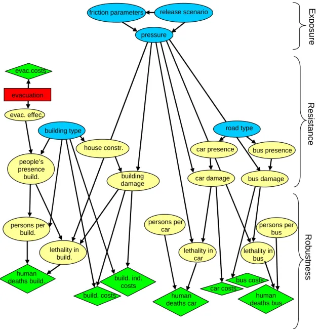
BN of the avalanche risk assessment developed in this study is given in Fig. 1. The arcs represent causal relations between the random variables. Those are characterized by their asso-ciated conditional probability tables, conditional on the states of any parent nodes that interact with it. The joint probability distribution of such a network is given as:

P (x) = P (x1, .., xn) = n

Y

i=1

P (xi|pa(xi)) (3)

where pa(xi), is a set of values of the parents of Xi. The

distribution of Xi given its parents may have any form, but

(4)

A. Grˆet-Regamey and D. Straub: Avalanche risk assessment linking Bayesian network to a GIS 913 bus costs pressure release scenario friction parameters

Robustnes

s

Resistance

evac. effec. people’s presence build. human deaths build. lethality in build. persons per build.

building type road type house constr.

building

damage car damage bus damage car presence bus presence

lethality in car

lethality in bus persons per

car persons per _bus

build. costs

build. ind.

costs _{car costs}

human deaths bus human deaths car

Ex

p

osure

evac.costs evacuation

Figure 1: Bayesian Network of avalanche risk assessment. The blue nodes represent the

input nodes, the yellow oval nodes represent the causal relations in the system, the red

boxes are the decision nodes, and the green rhomboid-shaped nodes are the utility

functions, characterizing the risk.

Fig. 1. Bayesian Network of avalanche risk assessment. The blue nodes represent the input nodes, the yellow oval nodes represent the causal relations in the system, the red box is a decision node, and the green rhomboid-shaped nodes are the utility functions, characterizing the risk.

the case where the nodes have discrete or Gaussian distribu-tions. Thus, we restrict ourselves to variables with discrete states in this study. BN can be extended to decision graphs by including decision nodes and utility nodes in the network. The decision nodes (Di) are used to set choices of

possi-ble protection measures and are represented as boxes. The rhomboids (Ui)represent the utility nodes; utilities are here

quantified in monetary values.

Figure 1 shows the BN for the risk assessment procedure arranged in accordance with the generic categories exposure, resistance and robustness. The blue nodes represent the input nodes, the yellow oval nodes are variables introduced to rep-resent the causal relations in the system and the

rhomboid-shaped nodes are the utility functions, characterizing the risk. The Appendix A gives the description of the content of the conditional probability tables corresponding to each node. The system exposure is expressed as the annual probability of occurrence of snow pressure at a defined location. The two nodes linked to the pressure node represent the posterior avalanche model applied in the risk assessment computations (Straub and Grˆet-Regamey, 2006). The system resistance is described by the probability that an avalanche damages buildings, cars or buses. One protection measure (evacua-tion) and its associated effectiveness are included as a sepa-rate box and a node in this part of the network to illustsepa-rate their effect on the risk. Several nodes model the relations

(5)

914 A. Grˆet-Regamey and D. Straub: Avalanche risk assessment linking Bayesian network to a GIS describing the robustness of the system, i.e. the consequences

of the impact of the avalanche on people or properties. The dependencies can be directly read from the network. Finally, the utility nodes define the expected costs as a function of the number of people killed and the physical damage to cars, buses, and houses. They are expressed in monetary terms.

BN enhance the utilization of evidence in the assessment of risks: Probabilities in the network are updated when new information is available. Finding the conditional distribution of a subset of the variables, conditional on known values for some other subset (the evidence) is the goal of inference. This conditional distribution is known as the posterior dis-tribution of the subset of the variables given the evidence e. For example, when the state of a variable is observed to be e, this information will propagate through the network and the joint probability of all nodes will change to its posterior:

P (x|e) =P (x, e)

P (e) (4)

Several algorithms exist to facilitate the updating of a prior probabilistic model using Bayes’ theorem (Murphy, 2001). We select the BN modelling shell Hugin (Hugin Expert, 2005) to solve the equations. We will use Bayesian inference to determine the joint probability distribution of the uncer-tainties associated with the avalanche model based on obser-vations of avalanches in the case study area.

2.1.2 Embedding BN into GIS

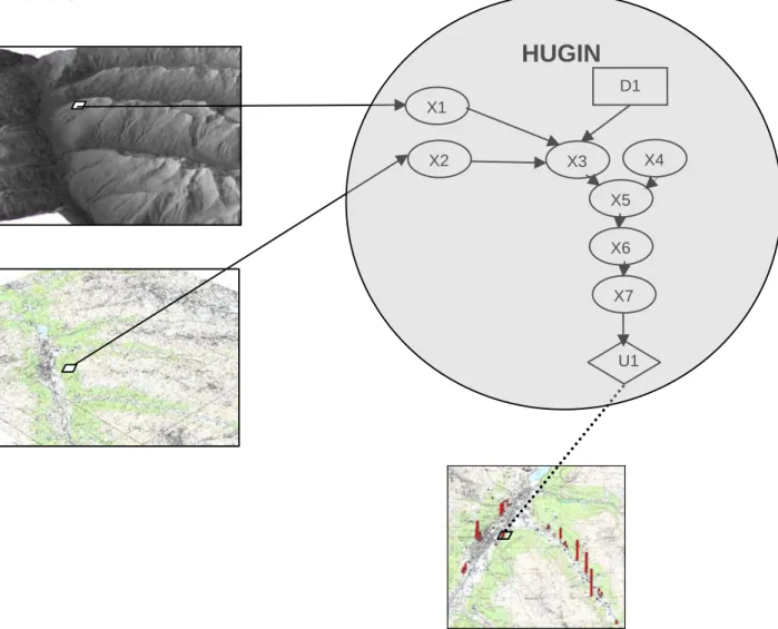
In order to estimate the risk on a cell basis, we integrate the BN created in the Hugin environment into ArcGIS 8.3 (ESRI, 2000). The HUGIN API is provided in the form of a library that can be linked to the Visual Basic programming language (Aitken, 1998). Using ESRI’s MapObjects 2.2 ActiveX com-ponents, the objects contained in the library can be called using the Visual Basic platform available in the ArcGIS en-vironment. Figure 2 shows the modelling framework, which is run for each of the 5 m×5 m raster cells of the case study area as follows:

1. The input nodes of the BN are initialized with values provided by spatially explicit datasets. The arrows be-tween the maps and the input nodes of the BN in Fig. 2 illustrate how the BN retrieves the values of the vari-ables from the datasets at each location. For example, the input nodes “building type” and “road type” (see Fig. 1) receive information about the location and the type of building and road at each location from a land-use map. The digital elevation model (DEM) provides information used in the avalanche model to calculate values used as evidence for the conditional probabil-ity tables of the “friction parameter” and the “pressure” nodes.

2. For each cell of the case study area, the evidence pro-vided by the spatially explicit datasets is propagated

through the BN. This process is entirely conducted within the Hugin shell, which supplies the mathemat-ical algorithms.

3. The main output of the BN is the annual risk for each cell expressed in monetary terms. These output values are provided in the ArcGIS environment and can imme-diately be drawn in maps.

2.1.3 Avalanche modelling

The probabilistic avalanche hazard modelling is presented in details in Straub and Grˆet-Regamey (2006). Here, we pro-vide only an overview.

The model is based on a two-dimensional avalanche dy-namic program, the 2D (Gruber, 1999). The AVAL-2D identifies the sizes of avalanche release zones, predicts run-out distances, flow velocities and impact pressures of dense snow avalanches. The sizes of the avalanche release zones are determined based on terrain characteristics and fracture depths. Snow fracture depths are built upon statis-tical analyses of maximum snow accumulation for three-day periods over the historical record (Salm et al., 1990). As these records only exist for about 60 years, the estimates of snow accumulations for events with a larger return pe-riod are extrapolated from the statistical record applying ex-treme value statistics. The fracture depths are adapted to slope and altitude based on Burkard and Salm (1992). The flow simulation model employs a “Voellmy-fluid” flow law, which assumes small shear strains in the flow body. Flow resistances, given by a dry-Coulomb type friction (µ) and a velocity squared friction (ξ ), are assumed to be concen-trated at the base of the avalanche. The latter is here mod-elled as a deterministic parameter, with different values for different slope angles, topographical classifications (such as open, confined, gully or flat) and surfaces (e.g., a value of 400 m2/s is assumed in forest areas). The values of µ are modelled by groups of stochastic variables, whose proba-bilistic model is obtained through Bayesian inference from observed avalanches recorded yearly from 1950 to 2003 in the winter reports of the SLF (unpublished data, SLF Davos, Switzerland).

The output of the avalanche hazard analysis is a proba-bilistic model of the annual maximum of the pressure P at any location. The AVAL-2D establishes a database with the calculated pressure at each cell as a function of the friction parameters and the release scenario. In combination with the joint probabilistic model of the friction parameters and the release scenarios, this represents a complete probabilis-tic model of P , which then serves as input variable to the rest of the risk assessment. As discussed in Straub and Grˆet-Regamey (2006), we do not include the influence of errors in the numerical avalanche model in an explicit manner.

(6)

A. Grˆet-Regamey and D. Straub: Avalanche risk assessment linking Bayesian network to a GIS 915 X3 X4 X5 X6 X7 U1 X1 X2

HUGIN

ArcGIS 8.3

D1

Figure 2: Illustration of the integration of a BN created in Hugin into ArcGIS 8.3

Fig. 2. Illustration of the integration of a BN created in Hugin into ArcGIS 8.3.

2.1.4 Uncertainty analysis

BN represent uncertainty by means of conditional and un-conditional probability tables. For example, the node repre-senting building damages describe the probability of differ-ent degrees of damages for given building types and given snow pressure. By solving the BN presented in Fig. 1, the uncertainties in the different nodes are propagated through the network and allow the determination of the distribution of the expected cost with respect to these uncertainties.

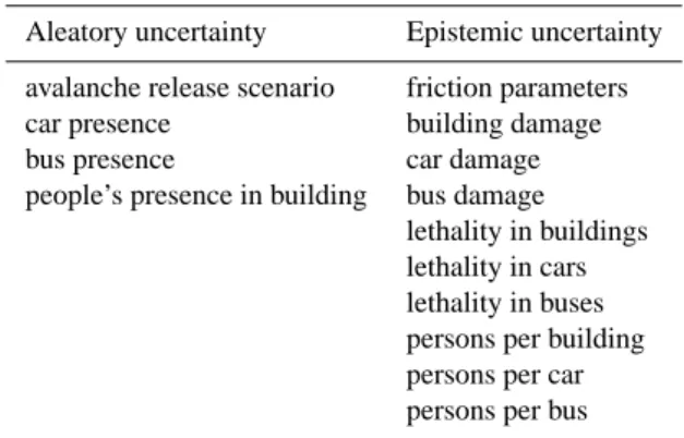
One of the advantages of using BN in risk assessment is that it facilitates determining which uncertainties should be reduced in order to increase confidence in the model. Not all uncertainties, however, can be decreased by an increase in knowledge. While aleatory uncertainties are inherent to a system and cannot be reduced by more detailed information (Parry, 1996), epistemic uncertainties result from incomplete knowledge of the object under investigation and may be

re-duced as more knowledge about the processes and parame-ters used in the model is obtained. Assigning the uncertainty sources of our model into these two classes is not always straightforward as in some cases no clear distinction between natural variability and lack-of-knowledge can be made. We will only incorporate epistemic uncertainties in the analysis, as these reflect our confidence in the model. Table 1 lists all the uncertainty sources in our BN and highlights the ones that we consider as epistemic.

To represent the epistemic uncertainty in the analysis, we determine the upper (u) and lower (l) bounds of the 95% Bayesian credible interval (sometimes also interpreted as confidence interval) for the total cost at each location. These upper and lower bounds are calculated from the distribution of the total cost CT Eas:

u = F_C−1

T E(0.975) (5)

l = F_C−1

(7)

916 A. Grˆet-Regamey and D. Straub: Avalanche risk assessment linking Bayesian network to a GIS

Table 1. Sources of uncertainty in the risk assessment model sep-arated into aleatory and epistemic uncertainty. Only the epistemic uncertainty is considered in the uncertainty analysis.

Aleatory uncertainty Epistemic uncertainty avalanche release scenario friction parameters car presence building damage bus presence car damage people’s presence in building bus damage

lethality in buildings lethality in cars lethality in buses persons per building persons per car persons per bus

With F_C−1

T E(p)being the inverse of the cumulative proba-bility distribution function of the total cost. The probaproba-bility distribution of CT E is obtained by calculating the total cost

for given values of the input variables at each location and by performing the expectation operation with respect to all aleatory uncertainties XA:

CT E =EXA[CT]

In a similar way, the aleatory uncertainties may be analysed, in particular the uncertainties regarding the avalanche release scenarios. The distribution of the total cost with respect to these uncertainties is of utmost importance for the planning of mitigation actions for extreme events.

2.1.5 Sensitivity analysis

Another way to establish the effect of the uncertainty associ-ated with the distribution of the variables used in the BN is to conduct a sensitivity analysis. In the present context, it is useful to determine which variables have the largest impact on the uncertainty in the total cost in order to economize re-sources when improving the model. The Shannon measure of mutual information provides a measure for ranking infor-mation sources (Shannon and Waver, 1949; Pearl, 1988). It is an indicator for the overall contribution of all the variables toward reducing the uncertainty in a target variable (T). It is based on the assumption that the uncertainty regarding any variable X characterized by a probability distribution P(x) can be represented by the entropy function:

H (X) = H (xi, ..., xn) = − n

X

i=1

P (xi)log(xi) (7)

Based on Eq. (7) Shannon’s mutual information, which is interpreted as the total uncertainty-reducing potential of X, is defined as (Pearl, 1988): I (T , X) = H (T ) − H (T |X ) = − n X i=1 m X j =1 P (tj, xi)log P (tj, xi) P (tj)P (xi) (8) Here, the target variable (T ) is the total cost of the avalanche hazard in monetary terms, CT. To compute this quantity

us-ing the BN, we combine all utility nodes into one probabil-ity node with states corresponding to the monetary values. The variables X include all the variables described in the BN given in Fig. 1.

2.2 Risk assessment using the “traditional approach” The approach traditionally applied for risk analysis is also based on Eq. (1) (e.g. Wilhelm, 1997). We multiply the prob-ability of each avalanche release scenario by the value of the object exposed to the hazard, the probability of exposure, and the vulnerability. In this study, the results of the AVAL-2D provide snow pressures at each location. These data points are linked to the damage potential using GIS. The data used in the traditional approach is the same as the data used in the BN approach, and is described in detail in Appendix A. But, as opposed to the BN approach, the risk is computed from the expected value of each random variable, thus ig-noring the probability distribution of the variables and their joint probability distribution. In other words, we replace all probability distributions of the random variables by the mean probabilities and calculate separately the risk for each build-ing and road type for a given avalanche release scenario. If all the relations among the variables in the BN were linear (e.g. if the lethality in buildings was a linear function of the building damage), then the BN approach would lead to the same results as the traditional approach.

For example, we estimate the building damage costs of a one-family house exposed to a 30-year avalanche release scenario given a snow pressure between 20 kPa and less than 30 kPa by multiplying the probability of a 30-year avalanche release scenario (0.03) with the probability of damage (0.74) and a building value of 1.07 Mio CHF, which gives a risk of 23 000 CHF. Using the BN approach, we introduce an un-certainty in the variable “building damage” by adding a state “some damage”. The risk calculated using the BN amounts then to 17 300 CHF.

Authors applying the traditional approach in avalanche risk assessment often approximate modelling uncertainties by means of deterministically defined buffer zones of the avalanche pressure zones. This approach was used, for ex-ample, to estimate uncertainties related to the damage poten-tial in the Landschaft Davos by assessing the probable maxi-mum loss (e.g. Fuchs et al., 2005; Br¨undl et al., 2006), which would correspond to some fractile value of the distribution of

CT in our approach.

2.3 Case study and data sources

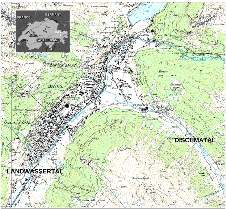
The study area is the “Landschaft Davos”, a commune in the eastern part of the Swiss Alps. The area consists of a

(8)

A. Grˆet-Regamey and D. Straub: Avalanche risk assessment linking Bayesian network to a GIS 917

DISCHMATAL

LANDWASSERTAL

Figure 3: The commune of Davos, covering totally 254 km

2

, is located in the eastern part

of Switzerland. The Landwassertal is the main valley, the Dischmatal is a hardly

populated SE-oriented side-valley.

Fig. 3. The commune of Davos, covering totally 254 km2, is located in the eastern part of Switzerland. The Landwassertal is the main valley, the Dischmatal is a hardly populated SE-oriented side-valley.

NE-SW-oriented main valley (Landwassertal) and four SE-NW-oriented valleys. The Landschaft Davos has always been an avalanche-prone area. The susceptibility of this area to avalanche damages is illustrated by the facts that the altitude of the valley bottoms is at 1400–1600 m above sea level, and highest peaks are over 3000 m above sea level, approximately 40% of the precipitations fall as snow, and, as a general rule, a closed snow cover is found from beginning of November to the end of May. In 2000, approximately 13 000 inhabi-tants lived in Davos, and up to 45 000 tourists were present during winter time (BfS, 2001). In this study, we will

specif-ically focus on the “Landwassertal” and a sparsely populated sivalley, the “Dischmatal” (Fig. 3). The two areas are de-lineated based on a valley length of 6 km, and the surface encompassing all avalanche release areas potentially threat-ening these valley segments.

Main spatially explicit data sources include the vector25 dataset based on the National Map 1:25 000 (Swisstopo, 2003), which provides the locations and types of roads and buildings on a resolution of 5 m×5 m. A detailed forest cover map with forest structures on a 5 m×5 m raster based on aerial photographs from 1950 and 2000 was provided by

(9)

410’000CHF/year

Figure 4: Total annual risk including fatalities and property damages in the Davos area.

Fig. 4. Total annual risk including fatalities and property damages in the Davos area.

Lardelli (2003). Topographical variables are obtained from the 25 m DEM (DEM25, Swiss Federal Office of Topogra-phy) and interpolated to a 5 m×5 m raster using the proce-dure described in Gruber (1999).

Other values used in the risk assessment procedure are based on literature data or were obtained by calculations. Appendix A summarizes the source and values of the data in-cluded in the nodes of the BN. Gaussian distributions based on expert knowledge are used to model the variables and re-lations for which no factual information is available. The probability distribution of each variable reflects its degree of uncertainty. Thus, it is necessary to consider all the available

information about the distribution of each variable. These values can be updated in a later step knowing the importance of their influence on the risk, which is investigated in the sen-sitivity analysis.

3 Results

3.1 Risk calculations

Annual risks calculated using the BN in the section consid-ered of the Landwassertal (3.1 Mio. CHF) exceed the annual

(10)

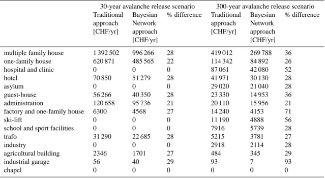
Table 2. Comparison of the annual risk given a 30-year and a 300-year avalanche release scenario in a section of the Landwassertal estimated using the traditional approach and a Bayesian Network.

30-year avalanche release scenario 300-year avalanche release scenario Traditional Bayesian % difference Traditional Bayesian % difference approach Network approach Network

[CHF/yr] approach [CHF/yr] approach [CHF/yr] [CHF/yr] multiple family house 1 392 502 996 266 28 419 012 269 788 36 one-family house 620 871 485 565 22 114 342 84 892 26 hospital and clinic 0 0 0 87 061 42 080 52 hotel 70 850 51 279 28 41 971 30 130 28 asylum 0 0 0 29 020 21 040 28 guest-house 56 266 40 350 28 23 330 14 953 36 administration 120 658 95 736 21 20 110 15 956 21 factory and one-family house 6300 4568 27 14 240 4153 71 ski-lift 0 0 0 11 190 4888 56 school and sport facilities 0 0 0 7916 5739 28 trafo 31 290 22 685 28 5215 3781 27

industry 0 0 0 2918 2114 28

agricultural building 2346 1701 27 484 345 29 industrial garage 56 40 29 93 7 93

chapel 0 0 0 0 0 0

risks in the section of the Dischmatal (1.7 Mio. CHF) by far (Fig. 4). The difference is mainly due to larger number of objects exposed to avalanches in the Landwassertal. The col-lective risk on roads is negligible in both valleys, amounting to 9500 CHF/year in the Landwassertal and 10 900 CHF/year in the Dischmatal. This is because in the Landwassertal, only a few road segments are exposed to risk, in the Dischmatal, the traffic frequency is low. Evacuation measures are calcu-lated to reduce the risk by 10% in the Landwassertal and 30% in the Dischmatal. We are, however, not considering risk ac-ceptance criteria for highly exposed individuals such as road workers and rescuers for which specific presence probabili-ties would have to be assessed.

BN cannot only be used to estimate risk in a spatially ex-plicit manner. They allow also the computation of the total annual risk in a region as associated with the different snow conditions, here represented in a discrete manner through the different release scenarios, as illustrated in Fig. 5. It is ob-served that the decrease in annual risk under larger and rarer avalanche events is gradual in the Dischmatal. In contrary, the low risk related to smaller avalanche events (the sce-nario corresponding to an assumed 10 years return period) in the Landwassertal reflects the fact that frequent but smaller avalanches do not reach highly populated areas.

Risk calculated using the traditional approach (6 Mio. CHF in the section of the Landwassertal) is 50% higher than the risk computed using the BN. The difference is mainly due to the probability distributions introduced in the vari-ables “building damage” and “lethality in building”, which

0 200,000 400,000 600,000 800,000 1,000,000 1,200,000 1,400,000 1,600,000 1,800,000

10year 30year 100year 300year

Landwassertal Dischmatal Total risk [CHF/ y ear ]

Avalanche release scenario

Figure 5: Distribution of the total annual risk in the Landwassertal and the Dischmatal for different avalanche release scenarios.

Fig. 5. Distribution of the total annual risk in the Landwassertal and the Dischmatal for different avalanche release scenarios.

influence the monetary consequences. Table 2 illustrates this difference in costs by building categories under the 30-year and the 300-year avalanche release scenario. Risks in one-and multiple-family houses, which are by one-and large at risk in the case study area, are the main drivers of this difference. Furthermore, these results confirm the findings presented in Fig. 5, where the 30-year avalanche release scenario causes more damage than the 300-year avalanche release scenario. In Fuchs and McAlpin (2005), the maximum probable loss for the area was estimated as amounting to 714 Mio. Euro using building insurance values.

(11)

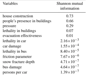
Table 3. Shannon mutual information I (CT, X), Eq. (7), with CT

as the total cost of the avalanche hazard, and X, all variables influ-encing CT.

Variables Shannon mutual information house construction 0.73 people’s presence in buildings 0.66 pressure 0.29 lethality in buildings 0.07 evacuation effectiveness 0.01 lethality in car 2.16×10−3 car damage 1.55×10−4 lethality in bus 8.40×10−5 friction parameter 7.67×10−6 snow fracture depth 4.71×10−7 bus damage 4.64×10−7 persons per car 1.39×10−7

All nodes not listed in this table have entropy reduction values of 0.

3.2 Uncertainty and sensitivity analyses

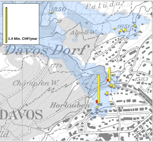
The uncertainty analysis yields Bayesian credible intervals for the overall costs, including all sources of epistemic un-certainty presented in Table 1. The maximum credible in-terval calculated from these uncertainty distributions is large (1.4 Mio. CHF) compared to the maximal expected cost of 235 000 CHF. As the intervals are relevant on the scale of buildings, Fig. 6 shows a credible interval map of a selected area in the Landwassertal. Uncertainties related to costs on roads were not represented as the costs are negligible com-pared to those of buildings. As all the lower bound values lie between 0 and 1000 CHF, they are not represented in Fig. 6. A comparison of the expected costs with the upper credible interval allows assessing the confidence in the results and the areas of greatest potential error. A map of expected cost val-ues used alone would give a false impression of precision: Risk values located at the border of the avalanche run-out zones have large confidence intervals, pointing to the large uncertainties in the estimation of the costs at these locations, and showing that a more reliable calculation of the avalanche pressures are crucial for reducing the uncertainty in the risk assessment. Furthermore, in zones affected mainly by low pressure avalanches, uncertainties are larger for light weight construction buildings such as agricultural buildings because of the uncertainties related to the size of the damage (“some damage” or “total damage”) of these buildings under low avalanche pressures. The fact that the pressure and the house construction nodes are two main sources of uncertainty is confirmed in the sensitivity analysis.

Based on the sensitivity analysis, the variables “house con-struction” and “people’s presence in buildings” are identi-fied as having the greatest influence on the total cost of the

avalanche hazard (Table 3). Next most influential variable is the pressure node. As the source of uncertainty of the vari-ables “house construction” and “people’s presence in build-ings” is epistemic, this result suggests that decision-makers should prioritize local data collection efforts on these vari-ables rather than on other varivari-ables listed in the BN. The un-certainty in the pressure node can be reduced using observed data as described in the next section.

3.3 Model improvement

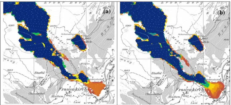
As the avalanche pressure node was identified as having a large influence on the cost values, we applied Bayesian in-ference to determine a probabilistic model of the variables influencing the calculated avalanche pressure using observa-tions of past avalanches (Straub and Grˆet-Regamey, 2006). According to the BN presented in Fig. 1, we are thus in-cluding uncertainties related to the physical parameters, and the assumptions made in the release scenario. Figure 7 shows a section of the Landwassertal with the annual prob-ability that an avalanche occurs using the original hazard model and the improved Bayesian model. The original model predicts a larger amount of shorter avalanches, whereas the posterior model predicts fewer but larger avalanches. This pattern is reflected in the risk values amounting to 3.1 Mio. CHF for risk in buildings and on roads using the original avalanche hazard model and 6.5 Mio. CHF under the improved Bayesian probabilistic model. In the original avalanche hazard model, the parameters used in the AVAL-2D were based on expert information (Gruber, 1999); in con-trary, the parameters in the improved avalanche hazard model were determined using Bayesian inference based on the ob-servation of past avalanches.

4 Discussion

BN applied to natural hazards, as described in this paper, has a number of specific advantages over the traditional ap-proach, especially when operated within the context of a GIS. Primarily, it allows for a consistent modelling of the risk arising from natural hazard. We show that the organization of the risk assessment procedure into a BN supports a structured approach to the interdisciplinary task requiring information from different specialist fields. For example, Fig. 1 shows the complexity of the factors involved in natural hazard risk assessment: The modelling of exposure, usually carried out by natural scientists, the assessment of system resistance as well as the robustness generally performed by engineers, and the monetarisation of the damages involving economists are assembled into a single model, which facilitates the commu-nication between the experts. If specialists identify variables which might have an impact on the risk but are missing data, they still can include them into the structure of the network leaving them uninstantiated. If at a later stage information

(12)

1.4 Mio. CHF/year

Figure 6: Bayesian credible intervals map. The red bars represent the expected cost value

at each location; the yellow bars are the upper bound values of the credible interval. The lower bound values are not represented as they all lie between 0 and 1000 CHF. The grey areas represent the avalanche extent under a 300-year scenario.

Fig. 6. Bayesian credible intervals map. The red bars represent the expected cost value at each location; the yellow bars are the upper bound values of the credible interval. The lower bound values are not represented as they all lie between 0 and 1000 CHF. The blue areas represent the avalanche extent under a 300-year scenario.

becomes available regarding these variables, it can then sim-ply be incorporated in the procedure.

Moreover, the integration of the probabilistic approach into a GIS allows quantifying and visualizing uncertainties in a spatially explicit manner, which is a basis to provide credi-ble information to planners. We show that, in the case study area, the risks estimated using a traditional risk approach are approximately 50% higher than the risks estimated using the BN. Uncertainties are large at the border of the avalanche run-out areas and are visualized in terms of credible inter-vals of the overall cost values (Fig. 6). Such maps thus allow objectively expressing confidence in the model results and visualizing its geographical variation.

Another advantage of using BN in natural risk assessment is the possibility to identify the variables causing large un-certainties in the results. In this study, we examine the dif-ferent sources of model uncertainties, and identify uncertain-ties related to the house construction, people’s presence in buildings, and the pressure variables as having the largest im-pact on the costs. By improving the avalanche model using Bayesian inference (Straub and Grˆet-Regamey, 2006) we see that the calculated risk increases by 34%. Such finding is

rel-evant for land-use planning activities such as hazard maps, as uncertainties in avalanche run-out areas can have a large im-pact on decision-making, especially in view of the increas-ing pressure to build into the near boundary of the endan-gered areas. By explicitly addressing these uncertainties, the BN approach allows quantifying their effects and facilitates identifying where future model improvements and data col-lection efforts should be concentrated. For example, we find that by improving the avalanche run-out model, collecting more data on people’s presence in buildings and vulnerabili-ties of buildings to avalanche pressure, confidence in the risk assessment results can be increased.

Yet, as the causal relationships between the variables in-fluence the results, it is important that the design of the net-work is discussed in an early planning step with specialists and decision-makers in order to include the important fac-tors in the analysis. Here, we did not include nodes describ-ing the comprehensive valuation of indirect costs. We sim-ply added a percentage of the building costs for quantify-ing indirect consequences based on the literature. A detailed analysis of the indirect costs including demographical, en-vironmental, medical, psychological, social and economical,

(13)

(a)

_(b)

Figure 7: Annual probability that an avalanche occurs, as evaluated with the prior model

(a) and the posterior model (b) model. The annual probabilities range from 2.5*10

-9

(brown) to 0.15 (blue).

Fig. 7. Annual probability that an avalanche occurs, as evaluated with the prior model (a) and the posterior model (b) model. The annual probabilities range from 2.5×10−9(brown) to 0.15 (blue).

structural and lifeline, and historical consequences (Faizian et al., 2004) may increase the risk considerably. Furthermore, other uncertainty factors especially related to the GIS data such as the vector25 dataset or the DEM could also be in-cluded in such analysis; thus providing an approach to com-municate error in spatial databases and study their impact on risk analysis.

The proposed framework offers many possibilities for fur-ther development in regard to the assessment and presenta-tion of the spatial and temporal distribupresenta-tion of the risk. In its present version, the BN is evaluated for each cell individu-ally, and thus only the risks and the credible intervals of the costs at each location are assessed. The spatial and temporal dependency structure of the risk is not evaluated. This de-pendency structure is of eminent importance for the planning of mitigation actions as well as for the inclusion of societal follow-up consequences. A small illustration of this aspect is given in Fig. 5, showing the distribution of the risk under different release scenarios: Objects in the Landwassertal are threatened by less frequent but much larger events compared to objects in the Dischmatal. However, this example is based on the simplifying assumption that the release scenarios are fully independent for the entire area (clearly an unrealistic assumption). Also, other dependencies of the variables in the model are not considered, e.g. the occupancy of different houses is clearly not independent, as the regional economy is dominated by tourism and thus introducing a common tem-poral fluctuation in housing occupancy. These spatial and temporal dependencies can be included by combining indi-vidual BN in the model to one single model. As long as

the individual BN are only related through common parent nodes, such a combination is computationally tractable.

If applied for the purpose of defining mitigation action plans, BN integrated into a GIS can be extended to provide a tool for optimal risk based decision making. In this study, we only consider evacuation as protection measure and ignore all the protection measures actually in place at many loca-tions in the case study area. Investigating the effect of differ-ent protective actions on the risk values using the framework presented in this paper will be an important future applica-tion of the model.

5 Conclusions

Considering the importance of an explicit consideration of uncertainties, BN linked to a GIS are supportive for present-ing credible risk assessments to decision-makers. The ap-proach unifies human expertise and quantitative knowledge in a coherent framework, which overcomes a major limita-tion of previous approaches; thus enhancing the understand-ing of the interdependencies of the involved processes and decisions. Furthermore, confidence intervals represented in a spatially explicit manner support the spatial interpretation of the risk. Lastly, as BN support modelling of the various in-terdependencies caused by common influencing parameters, such an approach might also have a large potential for link-ing different natural hazard risks in a slink-ingle system, which is worthy of further investigation.

(14)

Table A1. Values used in the BN nodes, organized into the generic categories exposure, resistance and robustness. Node # states Description of states Source of probability distribution

E xposu re Avalanche release scenario 5 1 year/10years/30 years/100 years/300 years

Direct function of the corresponding return period (Straub and Grˆet-Regamey, 2006): 0.89, 0.06, 0.03, 0.015, and 0.005

Friction parame-ters

9 µ1, µ2, µ3, µ4, µ5, µ6,

µ7, µ8, µ9

Following Straub and Grˆet-Regamey (2006)

Pressure 5 0 kPa

>0 kPa and <=3 kPa

>3 kPa and <=10 kPa

>10 kPa and <=20 kPa

>20 kPa and <=30 kPa

>30 kPa

Deterministic relations, calculated with AVAL-2D as a function of the friction parameters and the release sce-narios.

Resista

nce

Building damage 3 yes/some/no For one-family and multiple -family house: Barbolini et al. (2004), Fig. 4;

otherwise Borter (1999), p. 125; added state “some damage” (90% of damage =“yes”).

Upslope buildings within the snow accumulation area were not accounted for the protection of buildings downslope.

Car damage 2 yes/no assumed 99% car damage under avalanche event Bus damage 2 yes/no assumed 99% bus damage under avalanche event Car presence 2 yes/no Presence =p* g*DTV/v*24 (Wilhelm, 1997), where

p ( presence probability) = 113 days/181 days g=0.025

DTV (average number of cars per day) = 100 on first class road; 5 on second class road, 1 on third class road, and 0 on fourth class road

v (average speed) = 50 km/h on first class road, and 30 km/h on other roads

Bus presence 2 yes/no Wilhelm (1997), where p=113 days / 181 days

DTV=2000 on first class road; 50 on second class road, 30 on third class road, and 20 on fourth class road v=50 km/h on first class road, and 30 km/h on other roads House construc-tion 6 agricultural building administration building one-family house multiple-family house armed concrete safety construction Borter (1999), p. 125

Building type 18 agriculture building, garage, one-family house, multiple-family house, administration, school, hotel, industry, hospi-tal , living and work, chair-lift, apparthotel, staff house restaurant, trafo, reservoir, shop, church, depot

Hard labeling based on location of buildings given by Ingenieurb¨uro Darnuzer, Davos, (unpublished data)

(15)

Table A1. Continued.

Node # states Description of states Source of probability distribution People’s presence

in building

2 yes/no presence =T* D/24*7 (Borter, 1999a, p. 64), where T is the average presence time in hours per day, D is the average presence time in days pro week

Road type 4 1. class road 2. class road 3. class road 4. class road

Hard labeling based on location of roads (Vector25 data, SWISSTOPO, 2003)

Evacuation effec-tiveness

2 Effective/non-effective Fuchs and McAlpin (2005)

Evacuation costs 1000 CHF per building based on amount of people evacuated, time for evacu-ation, frequency of evacuation per year, hourly rate of helpers. R ob ustn ess Lethality in build-ings

2 yes, no Barbolini et al. (2004), Fig. 5. For the category “some damage”, assumed 50% lethality of “total damage” Lethality in cars 2 yes, no Borter (1999a, p. 72) for pressures 0–3 kN, and

>21 kN. The other values are extrapolated from the val-ues of Borter (1999a)

Lethality in buses 2 yes, no Borter (1999a, p. 72) for pressures 0–3 kN, and

>21 kN. The other values are extrapolated from the val-ues of Borter (1999a)

Persons per build-ing

101 numeric: 0–100 Mean based on Wilhelm (1997); variance proportional to mean.

Persons per car 3 Numeric: 1, 1.6, 2 Mean based on Borter (1999a, p. 72); variance propor-tional to mean.

Persons per bus Numeric: 2, 20,50 Mean based on Borter (1999a, p. 72); variance propor-tional to mean.

Cost of human death

1 5 Mio. CHF Life Quality Index approach amounting according to Merz et al. (1995)

Cost of destroyed car

30 000 CHF assumed based on http://wdb.wardsauto.com/ar/auto average newcar price

Cost of destroyed bus 1 Mio. CHF assumed Cost of destroyed building Indirect costs of destroyed building Belongings: 24%, infrastruc-ture: 15%, socio-economic costs: 10% of building value.

Communal cadastral register (Davos commune, unpub-lished data)

Wilhelm (1997), pp. 230–236

Acknowledgements. We would like to thank U. Gruber from the

SLF for providing data and support for the AVAL-2D, as well as P. Bebi from the SLF and M. Faber from ETH for their suggestions on earlier versions of this paper. Thanks also to M. Schubert from ETH for presenting this study at a conference. This work was partly funded by the Marie Heim-V¨ogtlin Fellowship 3234-69265 of the Swiss National Science Foundation (SNF). The second author is supported by the SNF through grant PA002-111428.

Edited by: J. M. Vilaplana Reviewed by: two referees

References

Aitken, G. P.: Visual Basic 6 programming. Blue Book Fast-Paced Learning, Coriolis Technology Press, pp. 700, 1998.

Amendola, A., Ermoliev, Y., Ermolieva, T., Gitits, V., Koff , G., and Linnerooth-Bayer, J.: A systems approach to modeling catas-trophic risk and insurability, Nat. Hazards J., 21, 381–393, 2000. Ancey, C.: Monte Carlo calibration of avalanches described as coulomb fluid flows, Philosophical Transactions of the Royal So-ciety of London, Phil. Trans. R. Soc. A., 363, 1529–1550, 2004.

(16)

Ancey, C., Meunier, M., and Richard, D.: The inverse problem for avalanche-dynamics models, Water Resour. Res., 39, 1099– 1112, 2003.

Antonucci, A., Salvetti, A., and Zaffalon, M.: Hazard assessment of debris flows by credal networks, Technical report IDSIA-02-04, IDSIA, available online: http://www.idsia.ch/idsiareport/ IDSIA-02-04.pdf, 2004.

Aspinall, R.: An inductive modelling procedure based on Bayes’ theorem for analysis of pattern in spatial data, Int. J. Geographi-cal Information Systems, 6, 105–121, 1992.

Barbolini, M., Cappabianca, F., and Sailer, R.: Empirical estimate of vulnerability relations for use in snow avalanche risk assess-ment, Risk Analysis IV, available under http://www.leeds.ac.uk/ satsie/docs/mb vuln.pdf, 2004.

Barbolini, M., Cappabianca, F., and Savi, F.: A new method for estimation of avalanche distance exceeded probabilities, Surveys in Geophysics, 24, 587–601, 2003.

Bayraktarli, Y. Y., Ulfkjaer, J., Yazgan, U., and Faber, M. H.: On the application of Bayesian probabilistic networks for earth-quake risk management, Paper presented at the 9th International Conference on Structural Safety and Reliability (ICOSSAR 05), Rome, Italy, 19–23 June 2005.

Bell, R. and Glade, T.: Quantitative risk analysis for landslides – Examples from B´ıdudalur, NW-Iceland, Nat. Hazards Earth Syst. Sci., 4, 117—131, 2004,

http://www.nat-hazards-earth-syst-sci.net/4/117/2004/.

Bfs (Swiss Federal Statistic Office): Statistisches Jahrbuch der Schweiz 2001, Zürich: Verlag Neue Züricher Zeitung, Zürich, Switzerland, 2001.

Borter, P.: Risikoanalyse bei gravitativen Naturgefahren – Fall-beispiele und Daten, Bundesamt f¨ur Umwelt, Wald und Land-schaft, Umwelt-Materialen Nr. 107/II, 1999.

Br¨undl, M., McAlpin, M. C., Gruber, U., and Fuchs, S.: Cost-benefit analysis of measures for avalanche risk reduction – a case study from Davos, Switzerland, in: Proc. Risk21 : Coping with risks due to natural hazards in the 21st century, edited by: Dan-nenmann, S., Ammann, W., and Vulliet, L., London, Taylor & Francis, ISBN 0-4154-0172-0, 2006.

Burkhard, A. and Salm, B.: Die Bestimmung der mittleren An-rissmaechtigkeit d0zur Berechnung von Fliesslawinen, Interner

Bericht Nr. 668. SLF, Davos, Switzerland, 1992.

Carrara, A. and Guzzetti, F. (Eds.): Geographical information sys-tems in assessing natural hazards, Kluwer Academic Publishers, Dordrecht, 1995.

Chen, K., Blong, R., and Jacobson, C.: Towards an integrated ap-proach to natural hazards risk assessment using GIS: With refer-ence to bushfires, Environ. Manag., 31, 546–560, 2003. Cruden, D. M. and Fell, R. (Eds.): Landslide risk assessment,

Proceedings of the International Workshop on Landslide Risk Assessment, 19–21 February 1997, Honolulu, Hawaii, A.A. Balkema, Rotterdam, The Netherlands, 1997.

Einstein, H. H.: Landslide risk assessment procedure, in: Proceed-ings of the 5th International Symposium on Landslides, 10–15 July 1988, Lausanne, Switzerland, 2, 1075–1090, 1988. ESRI (Environmental System Research Institute): ArcGIS 8.3.

ESRI INC, Redlands, CA, http://www.esri.com, 2000.

Faber, M. H., Kroon, I. B., Kragh, E., Bayly, D., and Decosemaeker, P.: Risk assessment of decommissioning options using Bayesian networks, J. Offshore Mechanics and Arctic Engineering, Trans.

ASME, 124, 231–238, 2002.

Faber, M. H. and Maes, M. A.: On applied engineering deci-sion making for society, Paper presented at the 9th International Conference on Structural Safety and Reliability (ICOSSAR 05), Rome, Italy, 19–23 June 2005.

Faizian, M., Schalcher, H. R., and Faber, M. H.: Consequence assessment in earthquake risk management using damage indi-cators, Paper presented at the 9th International Conference on Structural Safety and Reliability (ICOSSAR 05), Rome, Italy, 19–23 June 2005.

Ferson, S. and Ginzburg, L. R.: Different methods are needed to propagate ignorance and variability, Reliability Engineering and System Safety, 54, 133–144, 1996.

Fisher, P. F.: First experiments in viewshed uncertainty: The ac-curacy of the viewshed area, Photogrammetric Engineering and Remote Sensing, 57, 1321–1327, 1991.

Friis-Hansen, A.: Bayesian networks as a decision support tool in marine applications, PhD thesis, Technical University of Den-mark, 2000.

Fuchs, S., Keiler, M., Zischg, A., and Br¨undl, M.: The long-term development of avalanche risk in settlements considering the temporal variability of damage potential, Nat. Hazards Earth Syst. Sci., 5, 893–901, 2005,

Fuchs, S. and McAlpin, M. C.: The net benefit of public expen-ditures on avalanche defence structures in the municipality of Davos, Switzerland, Nat. Hazards Earth Syst. Sci., 5, 319–330, 2005,

Gruber, U.: Der Einsatz numerischer Simulationsmethoden in der Lawinengefahrenkartierung, Ph.D. Dissertation, Universität Zürich, Zürich, 1999.

Hincks, T., Aspinall A., and Woo, G.: An evidence science ap-proach to volcano hazard forecasting, Paper presented at the International Association of Volcanology and Chemistry of the Earths Interior (AVCEI), 2004.

Hugin Expert: HUGIN API reference manual, Version 6.4, Septem-ber 2005, available online: http://www.hugin.com, 2005. Hunter, G. J. and Goodchild, F.: Dealing with error in spatial

databases: A simple case study, Photogrammetric Engineering and Remote Sensing, 61, 529–537, 1995

Jensen, F. V.: Bayesian networks and decision graphs, Springer, New York, 2001.

Lardelli, C.: Dynamik und Stabilität von Lawinenschutzwäldern: Eine Luftbild- und GIS- gestützte Analyse, Diploma thesis Uni-verstät Zürich und SLF Davos, pp. 106, 2003.

Merz, H. A., Schneider, T., and Bohnenblust, H.: Bewertung von technischen Risiken – Beitr¨age zur Strukturierung und zum Stand der Kenntnisse. Modelle zur Bewertung von Todesfall-risiken, Vdf Hochschulverlag AG, ETH Z¨urich, Switzerland, pp. 175, 1995.

Morgan, G. C., Rawlings, G. E., and Sobkowicz, J. C.: Evaluating total risk to communities from large debris flows, in: Geotech-nique and Natural Hazards Symposium, BiTech Publishers, Van-couver, B.C., 225–236, 1992.

MunichRe: Topics Geo – Annual review: Natural catastrophes 2005, Order No. 302-04772, http://www.munichre.com, cited August 2006.

(17)

Sci-926 A. Grˆet-Regamey and D. Straub: Avalanche risk assessment linking Bayesian network to a GIS

ence and Statistics, 33, 2001.

Parry, G. W.: The characterization of uncertainty in probabilistic risk assessments of complex systems, Reliability Engineering and Systems Safety, 54, 119–126, 1996.

Pearl. J.: Probabilistic reasoning in intelligentsystems, Morgan Kaufmann Publishers, San Mateo, California, 1988.

Salm, B., Burkard, A., and Gubler, H.: Berechnung von Fliess-lawinen, eine Anleitung f¨ur Praktiker mit Beispielen, Mitt. Eid-gen¨oss. Inst. Schnee- Lawinenforsch., 47, 37 p., 1990.

Shannon, C. E. and Weaver, W.: The mathematical theory of com-munication, Urbana: University of Illinois Press, 1949. Stassopoulou, A., Petrou, M., and Kittler, J.: Application of a

Bayesian network in a GIS based decision making system, Int. J. Geographical Information Science, 12, 23–45, 1998.

Straub, D.: Natural hazards risk assessment using Bayesian net-works, Paper presented at the 9th International Conference on Structural Safety and Reliability (ICOSSAR 05), Rome, Italy,

19–23 June 2005.

Straub, D. and Grˆet-Regamey, A.: A Bayesian probabilistic frame-work for avalanche modeling based on observations, Cold Re-gions Science and Technology, in press, 2006.

Swisstopo: Vector25, Swisstopo, Wabern, Bern, http://www. swisstopo.ch, 2003.

Varnes, D.: Landslide hazard zonation: A Review of principles and practice, Unesco, Paris, 63 pp., 1984.

Wadge, G., Wislocki, A., Pearson, E. J., and Whittow, J. B.: Map-ping natural hazards with spatial modelling systems, in: Geo-graphic information handling: research and applications, Mather, P. M., John Wiley & Sons, Chichester, UK, 239–250, 1993. Wilhelm, C.: Wirtschaftlichkeit im Lawinenschutz. Methodik und

Erhebungen zur Beurteilung von Schutzmassnahmen mittels quantitativer Risikoanalyse und ¨okonomischer Bewertung, Mitt. Eidgen¨oss. Inst. Schnee- Lawinenforsch., 54, 1–309, 1997.