HAL Id: hal-02602550
https://hal.inrae.fr/hal-02602550
Submitted on 16 May 2020HAL is a multi-disciplinary open access archive for the deposit and dissemination of sci-entific research documents, whether they are pub-lished or not. The documents may come from teaching and research institutions in France or abroad, or from public or private research centers.
L’archive ouverte pluridisciplinaire HAL, est destinée au dépôt et à la diffusion de documents scientifiques de niveau recherche, publiés ou non, émanant des établissements d’enseignement et de recherche français ou étrangers, des laboratoires publics ou privés.
Christine Argillier, Nils Teichert, A. Sagouis, Mario Lepage, R. Schinegger, M.
Palt, S. Schmutz, P. Segurado, M.T. Ferrera, G. Chust, et al.
To cite this version:
Christine Argillier, Nils Teichert, A. Sagouis, Mario Lepage, R. Schinegger, et al.. Deliverable 5.A: Report on the comparison of the sensitivity of fish metrics to multi-stressors in rivers, lakes and transitional waters. [Research Report] irstea. 2015, pp.76. �hal-02602550�
Funded by the European Union within the
7th Framework Programme, Grant Agreement 603378. Duration: February 1st, 2014 – January 31th, 2018
Deliverable 5.A: Report on the comparison of the sensitivity of
fish metrics to multi-stressors in rivers, lakes and transitional
waters
Lead contractor: Irstea
Contributors: Christine Argillier, Nils Teichert, Alban Sagouis, Mario Lepage (Irstea), Rafaela Schinegger, Martin Palt, Stefan Schmutz (BOKU), Pedro Segurado, Maria Teresa Ferreira (ULisboa), Guillem Chust, Ainhize Uriarte, Angel Borja (AZTI)
Due date of deliverable: Month 18 Actual submission date: Month 18
Dissemination Level PU Public
PP Restricted to other programme participants (including the Commission Services) RE Restricted to a group specified by the consortium (including the Commission Services) CO Confidential, only for members of the consortium (including the Commission Services) X
Content
Content ... 3
Non-technical summary ... 5
Introduction ... 6
General approach ... 8
Multi-stressors analyses on rivers ... 9
Data and method ... 9
Fish sampling data/fish metrics ... 9
Pressure data/pressure combinations ... 11
Pairwise approach – random forests ... 12
Multiple combinatory approach – descriptive analysis ... 13
Prediction of combined effects ... 14
Results ... 14
Pairwise combinations - Proportion of explained variance ... 14
Stressor importance ... 15
Importance of pairwise interactions ... 17
Type of interactions – deviations from the additive effects ... 19
Stressor distribution and frequent stressor combinations ... 24
Reaction of metrics to single stressors and stressor combinations ... 26
Multi-stressors analyses on lakes ... 28
Data and method ... 28
Fish metrics ... 29
Environment and stressors ... 30
Modelling ... 32
Results ... 32
Effect of stressors on fish metrics of the European natural lakes ... 32
Interactions between stressors in European natural lakes ... 34
Effect of stressors of fish metrics in the French and Portuguese reservoirs ... 36
Interactions between stressors in French and Portuguese reservoirs ... 38
Data and methods ... 44
Stressor evaluation ... 45
Random forest model ... 47
Analysis of stressors on fish diversity ... 47
Simulation of EQR restoration benefits ... 47
Classification of interactions ... 48
Scheme of restoration ... 48
Results ... 49
Ecological responses for stressor descriptors ... 49
Effects of stressors on fish diversity ... 51
Simulation of EQR restoration benefits ... 52
Classification of interactions ... 53
Scheme of restoration ... 54
Discussion ... 56
Methodological considerations ... 56
Fish responses to stressors ... 57
Effects of frequent stressors on fish in rivers ... 57
Effects of frequent stressors on fish in lakes ... 58
Effects of frequent stressors on fish in estuaries ... 59
Interactions between stressors ... 60
Management purposes on estuaries ... 63
Appendix 1 ... 65
Appendix 2 ... 67
Appendix 3 ... 68
Non-technical summary
Aquatic ecosystems facing multiple stressors lead to challenging conditions for their management, as stressors can have additive, but also interactive effects on organisms, populations and communities. Accounting for these interactions is important in the assessment of the stressor’s impacts and to implement good restoration measures.
Using a comparable modelling approach and large environmental and fish databases, the combined effect of water quality problems and hydrological stressors were assessed, based on characteristics of fish assemblages observed in rivers, lakes, reservoirs and estuaries of Europe. The effects of non-native species in interaction with eutrophication and alteration of hydromorphology were also tested for fish assemblages of natural lakes and reservoirs.
We show that for all the water body types, water quality problems are a major threat that impacts fish assemblages. Similarly, alteration of the hydro-morphology explains a large part of the composition of river and estuarine fish assemblages. Conversely, we fail to demonstrate an effect of this stressor on the fish community of lakes and reservoirs, as sufficient data are not available yet. However, in these standing waters the introduction of non-native species can explain the variability of some characteristics of fish assemblages.
In a second step, we analysed the interactive effect of various stressors. Without interaction, the effect of two stressors on a fish assemblage characteristic corresponds to the sum of the individual effects. This additive effect was compared with the effects really observed in the assemblages to determine the type of interaction. The comparison was done for each fish assemblage characteristic impacted by stressors in each water body type. A large variability of multi-stressor impacts was observed, leading to higher or lower effects than expected in absence of interactions.
These results suggest to consider all potential stressors and interactions in the development of fish-based tools dedicated to ecological status assessment or restoration monitoring whatever the water body type is.
Introduction
To achieve long-term sustainable water resources management and the protection of European aquatic environment, the Water Framework Directive (WFD) was launched in 2000 (European Commission, 2000). To reach the ambitious objectives, i.e. the good ecological status/potential, monitoring of biological, physico-chemical and hydromorphological characteristics of all ground and surface water bodies (rivers, lakes, transitional- and coastal waters) was organized in the different countries of the EU. Currently, these monitoring programs support a large environmental data collection, allowing large-scale analyses of the relationships between biological communities and their environment.
In the framework of the WISER project (http://www.wiser.eu/), the response of biological/ecological characteristics of fish assemblages (i.e. fish metrics) to anthropogenic stressors was studied in rivers, lakes and estuaries. These studies aimed at understanding what the main factors involved in the organisation of fish assemblages are. Based on this knowledge, fish bioindicators/indices have then be developed by aggregating fish metrics in relation with abundance, composition and sensitivity of species, in order to assess the ecological status of the continental water bodies. However, in most of the cases, the analyses focused on the response of fish metrics to a single stressor or to several stressors but resumed by a single index value of pressure.
For rivers, Europe's first River Basin Management Plans (RBMPs) from 2009 indicate that 56% of European rivers failed to achieve good ecological status, as they are affected by a complex set of pressures resulting from e.g. urban and agricultural land use, hydropower generation and climate change (European Environment Agency [EEA], 2012). Along with increasing pressure placed on riverine ecosystems, both scientists and water resource managers need greater understanding of the relationships between multiple anthropogenic stressors and the response of the aquatic community, i.e. if they have synergistic, antagonistic or additive effects, to understand the impact on and the future management of aquatic ecosystem services (Allan et al., 2013). Research projects funded by the EU, e.g. FAME (Fish-based Assessment Method for the Ecological Status of European Rivers, FAME Consortium, 2004) and EFI+ (“Improvement and Spatial Extension of the European Fish Index”, EFI+ Consortium, 2007) investigated related issues. Based on the results of EFI+ project (EFI+ Consortium, 2007), Schinegger et al. (2012) first showed that (1) degradation of European rivers is widespread, (2) single water quality pressures (W) are not dominant, but (3) many European rivers are affected by hydromorphological pressures (HMC) or a combination of pressure types (W + HMC).
Similarly, in lakes eutrophication characterised by nutrient concentrations or indirectly by the intensity of non-natural land cover (agricultural and urban) in the catchment of the lake, is recognised as a major threat to achieve the good ecological status. Therefore, most of the bioindicators are dedicated to the assessment of this stressor and fish are often used for this purpose (Argillier et al., 2013; Kelly et al., 2012; Olin et al., 2013). Alteration of hydromorphology is also expected to affect fish communities notably through habitat and reproduction substrate diversity and availability (Drake
and Pereira, 2002). Introduction of non-native species, a frequent practice in standing waters (Cowx, 1998; Irz et al., 2004; Welcomme, 1988), highly impacts biodiversity and the ecosystem functioning (Garcia-Berthou and Moreno-Amich, 2000; Whittier and Kincaid, 1999) and can, as a consequence, modify the ecological status of the lakes (Gassner et al., 2003). However regarding these two stressors, clear pressure-impact relationships seem to be difficult to demonstrate by large scale analyses (Brucet et al., 2013). As a consequence, the effects of eutrophication, alteration of hydromorphology and introduction of non-native species in combination are seldom quantified. In estuaries (i.e. transitional waters), several modelling approaches have been conducted in previous studies to test the sensitivity of fish metrics to a pressure index or specific pressures. Despite the major effect of variables from the sampling and from natural features, most of metrics responded to the gradients of anthropogenic pressures using linear models (GLM, LM). Nevertheless, as for the others water body types, these approaches rarely considered the interaction between stressors and did not evaluate the relative contribution of each stressor.
Current challenges include using the large biological databases generated through the WFD monitoring surveys (http://www.eea.europa.eu/data-and-maps/data/wise_wfd) and for the intercalibration of methods (Birk et al., 2013), to identify and predict the effects of multiple stressors on ecosystems in order to help water managers prioritizing mitigation measures (Hering et al., 2015; Reyjol et al., 2014).
Systems facing multiple stressors are challenging conditions for management because stressors can have additive, but also interactive effects on organisms, populations and communities (Crain et al., 2008). The combined effect of multiple stressors was commonly assumed to be additive, i.e. equal to the sum of stressors’ individual effects acting in isolation. However, this model does not seem prevalent in ecological systems compared to antagonistic and synergistic interactions (Crain et al., 2008). Stressors can act in synergy when the combined effect of stressors is greater than the sum of the impacts of individual stressors, whereas antagonistic interactions occur when the combined effect of stressors is less than expected based on their individual effects (Folt et al., 1999). In these conditions, the ecological benefit resulting from efforts to reduce any stressors acting additively can be predicted on the basis of the knowledge of its individual effect, whereas interactive effects could produce some ‘ecological surprises’ (Paine et al., 1998). Although synergic interactions are expected to be more harmful for ecosystems because of accelerating system degradation, they also provide advantageous opportunities of restoration yielding larger overall benefits than if additive or antagonistic effects are involved (Crain et al., 2008; Piggott et al., 2015). Conversely, the efforts to mitigate stressors often not yield proportional benefits in systems where antagonistic interactions are prevalent, which is often considered as the “worst-case” scenario for ecosystem management (Brown et al., 2013; Folt et al., 1999; Piggott et al., 2015). The development of scheme for prioritizing management actions should thus consider the type and the strength of interactions (Halpern et al., 2008).
The present work is in the wake of the previous analyses conducted in the WISER project. More precisely, it is dedicated to:
- A better understanding of the combined effects of several stressors, on the fish metrics/indices identified as relevant to assess the ecological status of the water bodies. Indeed, water bodies seldom experience a single pressure and it is possible to improve the diagnosis on the ecological status taking into account a larger range of stressors. The stressors can act in interaction or not and impact different facets of the communities.
- The analysis of differences in fish communities responses to multi-stressors in rivers, lakes and estuaries taking into account the specificity of each water body type. Due to differences in ecosystem functioning between lentic and lotic waters and between freshwater and brackish waters, we can expect different responses of the communities to a same combination of stressors.
General approach
In the analyses conducted on rivers and lakes, a metric was defined as a measurable variable or process that represents an aspect of the biological structure, function, or other component of the fish community and changes in value along a gradient of human influence (Karr, 1999). In these studies, metrics tested are related to composition, abundance, sensitivity and size structure of fish communities. These metrics are based on taxonomic or functional guilds. In the analyses conducted on estuaries, some diversity metrics were included in the analyses of a French dataset. However, in estuaries, because sampling methods and strategies were very different from one country to another, calculation of metrics at the European scale is not sound. Therefore, the Ecological Quality Ratios (EQR) of the fish index in application in each country were calculated and used in the present work. The EQR defined as the ratio of the observed fish index value to the expected value under reference conditions was used. These indices are multi-metrics indices supposed to take into account the influence of natural environmental characteristics of estuaries on fish communities.
To achieve the objectives, whatever the water body type, Random Forests models (Breiman, 2001) were implemented to assess and rank the importance of pairwise stressor interactions. This machine learning approach allows freedom from normality and homoscedasticity assumptions and did not require previous data transformation (Mercier et al., 2010). It is suited to identify relevant predictors from a large set of candidate variables even though the number of observations is small (Strobl et al., 2007). The random forest algorithm generates a great number of decision trees involving two specific random features. The first one is a bootstrap resampling used to select approximately 63.2% of the whole dataset to build a given tree (‘in-bag’ data). The second one occurs at each decision node of the tree to select a random subset of predictors from which the predictor minimizing the mean squared error is retained to grow the tree. The remaining 36.8% of data not kept to grow the tree (i.e. ‘out-of-bag’ data) are used to provide independent estimations of the prediction error for each tree. The model estimates are obtained by averaging the predictions from all the individual regression trees of the forest. Using a large number of trees ensure that each metric had enough of a chance to be
included in the forest prediction process. The number of metrics randomly selected at each node was fixed at 5 and the minimum number of unique observations in a terminal node was also fixed at 5, as advised for regression analysis. As some predictors contain missing values, the imputation method developed by Ishwaran et al. (2008) was used to attribute data by randomly drawing values from non-missing in-bag data. The percentage of variance explained by the model was estimated based on the out-of-bag observations, which provided a reliable evaluation of the adjustment (i.e. goodness-of-fit). For all the water bodies, the importance of each stressor in the Radom Forest models, were computed using an approach based on Breiman-Cutler permutations (implemented in the “VIMP” function of “randomForestSRC” R package). For each tree, the prediction error on the OOB data is recorded and then for each stressor, OOB cases are randomly permuted and the prediction error is recorded. The variable importance (VIMP) is then defined as the difference between the perturbed and unperturbed error rate averaged over all trees in the Forest (Ishwaran, 2007). A measure of relative importance (%) expressing the proportion of each VIMP to the sum of VIMP of all stressors was then computed in order to compare the variable importance among different fish metrics.
Analyses were performed with the R statistical software (R Core Team, 2014) and the package ‘randomForestSRC’ (Ishwaran and Kogalur, 2014).
Multi-stressors analyses on rivers
Data and methodFish sampling data/fish metrics
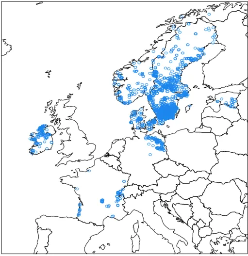
In total 3105 European fish sampling sites in 14 countries were available for our analyses, extracted from an extensive database (EFI+ Consortium, 2007). Sites were sampled by electrofishing (wading) considering European standards (C.E.N., 2003) and were associated with four fish assemblage types (FATs, i.e. Headwater streams, Medium gradient rivers, Lowland rivers and Mediterranean streams; Figure 1) based on fish community and environmental characteristics ((Schinegger et al., 2013; Trautwein et al., 2013).
Figure 1 - Spatial location of sites [n = 3105] and associated fish assemblage type (FAT’s according to Schinegger et al., 2013).
Overall, 20 fish metrics associated with six structural and functional types (biodiversity, habitat, migration, reproduction, trophic level and water quality sensitivity) were available for further analyses (Table 1), based on the findings of Schinegger et al. (2013), Trautwein et al. (2013) and Segurado et al. (2008) in terms of reaction to single and multiple stressors.
Table 1 - Fish metrics available for river analyses.
Metric name Definition Type Variants Direction
Nsp_all Total number of fish species, including
native and alien species. biodiv nsp decr/incr
HTOL_HINTOL Habitat degradation intolerance. hab dens juveniles
(<150mm) decr
HTOL_HTOL Habitat degradation tolerance. hab perc_biom incr
HabSp_RHPAR Preference to spawn in running waters. hab dens decr Repro_LITH
Fish spawn exclusively on gravel, rocks, stones, rubbles or pebbles, hatchlings are photophobic.
repro dens decr
Atroph_INSV Insectivorous species. troph nsp decr
Atroph_PISC Piscivorous species. troph perc_nsp decr
Atroph_OMNI
Food of adult consists of more than 25% plant material and more than 25% animal material. Generalists.
troph perc_biom, perc_nsp incr WQgen_INTOL In general intolerant to usual water quality
parameters. wq
biom, dens, perc_nsp,
pers_dens decr
WQgen_TOL In general tolerant to usual water quality
parameters. wq biom, nsp, perc_dens incr
WQO2_O2INTOL Tolerant to low Oxygen concentration.
More than 6 mg/l in water. wq biom, dens, perc_nsp decr WQO2_O2TOL Tolerant to low Oxygen concentration: 3
mg/l or less. wq perc_nsp incr
Pressure data/pressure combinations
Pre-classification of sites for anthropogenic stressors was available for 13 selected stressor variables (according to Schinegger et al., 2012 and Schinegger et al., 2013), to differentiate unimpacted sites from single- or multiple impacted sites (Table 2).
Table 2 - Stressor variables available for river analyses.
Stressor variable Abbreviation Description
Impoundment H_imp Natural flow velocity reduction on site due to impoundment Hydropeaking H_hydrop Site affected by hydropeaking
Water abstraction H_waterabstr Site affected by water flow alteration/residual flow
Reservoir flushing H_resflush Fish fauna affected by flushing of reservoirs upstream of site Hydrograph modification H_hydromod Seasonal hydrograph modification due to hydrological alteration
(water storage for irrigation, hydropower etc.)
Morphological alteration M_morph_instr Alteration of natural morphological channel plan form, cross section and instream habitat conditions
Embankment M_embank Artificial embankment
Flood protection M_floodpro Presence of dykes for flood protection Barriers upstream C_up Barriers upstream of site
Barriers downstream C_do Barriers downstream of site
Acidification W_acid Artificial acidification
Eutrophication W_eutroph Artificial eutrophication
Organic pollution W_opoll Pollution by organic substances
Pairwise approach – random forests
Random Forests models (Breiman 2001; see brief description of the method in the section General approach of this deliverable) were fitted using each one of the 20 river fish metrics as the response variable and the 13 stressors considered in this study as covariates. Fish Assemblage Type was also included as covariate in the models to control for its effect on the metric response to stressors. According to the cumulative out-of-bag (OOB) error rate as a function of number of trees, a forest of 1000 trees were overall adequate.
The importance of individual stressors was assessed following the method previously described (section General approach). Grown random forests were also used to identify and rank the potential importance of pairwise interactions for all pairs of stressors. This ranking was also based on Breiman-Cutler permutations (implemented for interactions in the “find.interaction” function of “randomForestSRC” R package) but in this case the paired VIMP was calculated instead, referred to as “paired” importance. This measure was then compared with the sum of VIMP of the individual stressors, referred to “additive” importance. A large positive or negative difference between 'Paired' and 'Additive' indicated an interaction worth pursuing in case the univariate VIMP for each stressor was reasonably large. The ranked absolute differences between Paired and Additive VIMP were computed to allow comparing the importance of each pair of stressors among metrics. A relative difference [(Paired – Additive) / Additive] was also computed as an alternative to compare interactions. Pairwise combinations that yielded fewer than 10 sites per pairwise category combination were discarded. Co-plot graphs were plotted for the most responsive metrics to visually
identify the most important interactions and assess whether the main deviations from additive effects corresponded either to synergistic or antagonistic interactions.
Multiple combinatory approach – descriptive analysis
Some fish metrics decrease in response to increasing anthropogenic stress (less fish of a guild leading to reduced density and biomass, disappearance of species) but in contrast, several others tend to increase, thus having a reaction in reverse direction, e.g. metrics associated with generalist and tolerant species (Schinegger et al., 2013; Trautwein et al., 2013). We used EQR to identify the degree of metric response between sites impacted by frequently occurring stressor combinations and unimpacted sites. EQRs were calculated for each individual site as follows:
Formula I:
EQR mean metricmetric
Where i = 1…3105
Formula I is applied for metrics expected to decrease under increasing number of stressors as well as metrics expected to increase under increasing number of stressors if they were recorded in percentage rates. For these percentage metrics, a proxy was calculated, based on the percentage not meeting the metric value (i.e. for percentage of species tolerant to habitat degradation, the percentage value not tolerant was considered) (Formula II).
Formula II:
EQR 100 mean metric100 metric
Where i = 1…3105
For metrics in absolute numbers, which are expected to increase with increasing number of stressors, the EQR is calculated as follows:
Formula III:
EQR
mean metric
metric mean EQR
Where i = 1…3105
These calculations are sensitive to FAT, i.e. separate mean metrics for the unimpacted sites were calculated for each of the four river types to which the metric at a given site of a particular river type is compared. This step was included to compensate for environmental effects that might influence the sampling site. FAT of impacted sites was predicted by the method developed by Schinegger et al. (2013) and Trautwein et al. (2013).
Prediction of combined effects
The combined effects of stressors were predicted from single stressors and were defined as deviation from reference condition by ecological quality ratio (EQR) according to Formula 3 (modified based on Coors and De Meester, 2008). Deviations of observed from predicted EQRs can then be interpreted in the following way: synergistic effects between pressures are indicated by a significantly stronger observed effect of the combined stressors than the predicted one (from single stressors), whereas an antagonistic effect is indicated by a significantly weaker value of observed value than predicted (Coors and De Meester, 2008). No deviation between observed and predicted EQRs can be interpreted as additive effect.
Results
Pairwise combinations - Proportion of explained variance
The proportion of the variance of fish metrics explained by the Random Forest models varied between 36.9% for the metric % of species intolerant to oxygen depletion (WQO2_O2INTOL_perc_sp; Fig. 2) and 5.3% for the metric abundance of rheophilic spawning
species (HabSp_RHPAR_dens; Fig. 2). For most metrics, FAT contributed approximately to half of
the total explained variance. Metrics with higher contribution of stressors to the explained variance tended to be also those with the highest total explained variance, and vice-versa. The five metrics with the highest contribution of stressors to the explained variance were: total abundance of juveniles
intolerant to habitat degradation (HTOL_HINTOL_dens_juv), % of species intolerant to oxygen depletion (WQO2_O2INTOL_perc_sp), total richness (NSp_all), % of omnivorous biomass
(Atroph_OMNI_perc_biom) and % of abundance of intolerant to general water quality degradation (WQgen_INTOL_perc_dens).
Figure 2 - Total percentage of variance explained by the Random Forest models for each metric. The contribution of FAT and stressors is also represented. Fish metrics are sorted by a decreasing order of
stressor contribution to the explained variance.
Stressor importance
Except for four metrics (WQgen_INTOL_biom, WQgen_TOL_biom, WQO2_O2INTOL_biom and Atroph_OMNI_perc_biom), FAT was the most important variable in the random forest models (Table 3, Figure 3). Among the ten metrics that had a higher share of explained variance by stressors, eutrophication was the most important stressor for four metrics, followed by organic pollution for three metrics, in-stream morphology alteration for two metrics and hydrograph modification for one metric (Table 3). These stressors, along with embankment and flood protection, were the stressors showing the highest median importance among the different metrics (Figure 3).
Table 3 – Relative variable importance (%) of each stressor in Random Forest models fitted for each fish-based metric. Metrics are sorted in a decreasing order of the contribution of stressor variables to the explained variance. Fish Metrics FAT C_ B_ s_d o C_ B_ s_u p H _hy dr omo d H _hy dr op H_im p H_ resfl us h H_ watera bst r M_ em ban k M _f lood pro M_ m or ph _i nst r W_aci d W _eu trop h W_ opol l Htol_Hintol_dens_juv 36.4 2.1 1.2 5.9 3.1 6.1 0.0 1.5 2.0 0.8 18.5 0.0 18.3 4.1 WQO2_O2INTOL_perc_sp 52.9 1.2 0.8 9.4 1.2 1.2 0.1 0.9 1.3 0.8 4.1 0.3 21.3 4.3 Nsp_all 46.2 0.2 2.9 7.3 0.5 0.4 0.6 1.3 2.3 12.5 3.9 0.7 5.7 15.5 Atroph_OMNI_perc_biom 13.9 0.7 0.5 20.5 1.9 5.4 -0.1 2.3 0.9 1.3 4.4 0.2 25.2 22.9 WQgen_INTOL_perc_dens 41.7 0.8 0.6 10.4 1.3 2.7 0.0 0.8 2.0 0.7 8.6 0.3 23.5 6.7 WQgen_TOL_n_sp 44.5 0.2 1.5 12.3 0.5 2.3 1.1 1.1 2.8 6.6 7.5 0.2 7.4 11.9 Y_MetO2INTOL 38.0 1.5 0.5 7.4 2.8 2.6 0.1 1.2 2.2 0.8 11.2 0.0 28.0 3.6 WQgen_INTOL_perc_sp 51.5 1.2 0.6 9.2 0.9 2.2 0.0 0.5 1.6 0.6 5.4 0.3 20.2 5.8 Atroph_INSV_nsp 43.4 0.4 3.4 2.6 0.5 0.5 0.5 2.1 3.5 17.9 4.3 1.3 2.4 17.3 Atroph_OMNI_perc_sp 49.6 0.8 0.3 7.3 0.3 1.3 0.2 1.4 1.9 1.2 14.2 0.6 12.0 8.9 HTOL_HTOL_perc_biom 39.3 0.5 0.7 10.0 0.5 4.0 0.0 0.4 2.4 0.8 7.9 0.0 11.7 21.6 WQgen_TOL_perc_dens 43.8 3.1 0.3 4.8 0.9 6.9 0.2 1.1 3.0 2.1 16.2 0.2 11.4 6.0 WQO2_O2INTOL_biom 16.1 2.8 3.9 14.4 2.9 -2.1 -0.2 0.6 8.3 29.7 3.6 0.4 14.9 4.7 WQO2_O2TOL_perc_sp 51.3 0.6 0.1 6.1 0.4 1.6 0.1 0.4 2.2 1.5 6.9 0.1 15.4 13.4 Atroph_PISC_perc_sp 51.7 5.1 0.5 2.5 3.2 2.1 0.0 6.1 10.7 1.4 3.4 0.4 1.8 11.2 WQgen_TOL_biom 10.6 7.5 2.2 6.0 -2.2 -2.8 0.0 7.7 5.4 8.4 6.1 0.1 16.2 34.8 WQO2_O2INTOL_dens 31.0 8.2 3.1 3.7 8.3 1.9 0.0 -0.2 16.3 7.6 4.1 -2.1 9.1 9.1 WQgen_INTOL_dens 39.4 2.6 6.3 7.9 12.2 6.5 0.1 0.9 4.8 1.9 5.5 0.0 11.5 0.4 WQgen_INTOL_biom 20.3 -1.6 2.7 4.8 6.3 -3.8 0.0 5.6 16.8 39.0 -0.5 0.4 0.8 9.4 HabSp_RHPAR_dens 19.1 2.8 14.2 4.6 13.4 -1.2 4.3 -2.1 7.5 4.7 8.2 0.2 7.8 16.5
Figure 3 – Boxplot showing the distributions of the relative stressor and FAT (Fish Assemblage Type) importance based on the random forest models for the eighteen metrics analysed.
Importance of pairwise interactions
The boxplots of Figure 4 show the overall importance of stressor interactions according to the Random Forest models, as measured by the ranked absolute difference between paired and additive VIMP values, for the 20 fish metrics. Eutrophication paired with organic pollution showed the overall higher relevance and simultaneously the lowest variability among metrics. Other important interactions included in-stream morphological alteration with eutrophication, in-stream morphological alteration with embankment, flood protection with eutrophication and impoundment with eutrophication.
Figure 4 - Boxplot showing the distributions of the ranked interaction importance of each pairwise combination of stressors, based on the random forest models for the twenty metrics analysed.
Type of interactions – deviations from the additive effects
The boxplot of Figure 5 shows the distribution of the relative difference between paired and additive importance in the Random Forest models, which expresses the deviations from the additive effects. The pressure pairs are sorted according to their rank importance for each metric. This figure shows that the rank position of each interaction does not always reflect the magnitude of the deviation from the additive effects, although there is a general trend for pairwise interactions with higher ranks to show more pronounced deviations from additive effects and vice-versa. Eutrophication paired with organic pollution also showed the highest deviations from additive effects. Other pairwise interactions with pronounced deviations from additive effects included impoundment with barriers downstream, in-stream morphological alteration with embankment, flood protection with embankment and in-stream morphological alteration with eutrophication.
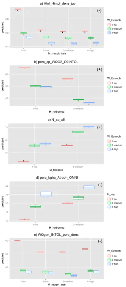
The response to the pairwise interaction that deviates the most from additive effects according to the random forest models (eutrophication and organic pollution) was explored with partial co-plots for the five most responsive metrics to stressors: total abundance of juveniles intolerant to habitat
degradation (HTOL_HINTOL_dens_juv; overall negative response to pressures; Fig. 6a), % of species intolerant to oxygen depletion (WQO2_O2INTOL_perc_sp; overall negative response to
pressures; Fig. 6b), total richness (Nsp_all; overall positive response to pressures; Fig. 6c), % of
omnivorous biomass (Atroph_OMNI_perc_biom; overall positive response to pressures; Fig. 6d) and % of abundance of intolerant to general water quality degradation (WQgen_INTOL_perc_dens;
overall negative response to pressures; Fig. 6e). The partial co-plots suggest that both synergistic and antagonistic interactions might be expected for this stressor pair, depending on the metrics. No relationship between the overall direction of the effect (positive of negative) and the type of interaction (synergistic or antagonistic) seems to occur. Synergistic effects - i.e. eutrophication tends to attenuate the effect of organic pollution and vice-versa - are predicted to three metrics (HTOL_HINTOL_dens_juv, NSp_all; Atroph_OMNI_perc_biom) and antagonistic effects – i.e. eutrophication tends to enhance the effect of organic pollution and vice-versa - are predicted for two metrics (WQO2_O2INTOL_perc_sp, WQgen_INTOL_perc_dens).
The co-plots of Figure 7 shows the simultaneous effects of other important pairwise interactions for each five most responsive metrics to stressors. For the metric total abundance of juveniles intolerant
to habitat degradation (HTOL_HINTOL_dens_juv) the random forest model suggests a potential
interaction between instream morphological alteration and eutrophication. According to the co-plot (Fig. 7a), eutrophication tends to attenuate the effect of instream morphological alteration and vice-versa, namely between the categories “no” to “low” of instream morphological alteration, suggesting an antagonistic effect. The same antagonistic effect for the same stressor pair is also suggested by the partial co-plot for the metric % of abundance of intolerant to general water quality degradation (WQgen_INTOL) (Fig. 7e). For metric % of species intolerant to oxygen depletion (WQO2_O2INTOL), the co-plot suggests a slight synergistic effect between hydrograph modification and eutrophication (Fig. 7b). A slight synergistic effect is also suggested by the co-plot between the partial effects of flood protection and eutrophication for the metric total richness
(Nsp_all) (Fig.7c). For metric % of omnivorous biomass (Atroph_OMNI_perc_biom), an antagonistic effect is suggested by the co-plot between the partial effects of hydrograph modification and impoundment (Fig. 7d).
In the case of the response of the total number of species a synergistic interaction is suggested by the partial co-plot of the simultaneous effects of eutrophication and organic pollution: an increase of eutrophication tends to accentuate the unimodal response to water pollution. The simultaneous response to the pair eutrophication and flood protection suggests also a slight synergistic effect: eutrophication tends to slightly enhance the effect of flood protection (Fig. 7a and 7b).
Figure 5 - Boxplot showing the distributions of the Relative difference between the sum of the individual importance values and the paired importance values for each pairwise combination of stressors, based on the random forest models for the eighteen metrics analysed. Values of relative difference that lie either in a more negative or more positive position represent potential interaction effects.
Figure 6 - Partial co-plots showing the simultaneous response of the five most responsive metrics to organic pollution (W_opoll) and eutrophication (W_eutroph). Plots marked with (+) suggest synergistic effects and those with (-) suggest antagonistic effects.
Figure 7 - Partial co-plots showing the simultaneous response of the five most responsive metrics to other important interactions according to the Random Forest models. Plots marked with (+) suggest synergistic effects and those with (-) suggest antagonistic effects.
Stressor distribution and frequent stressor combinations
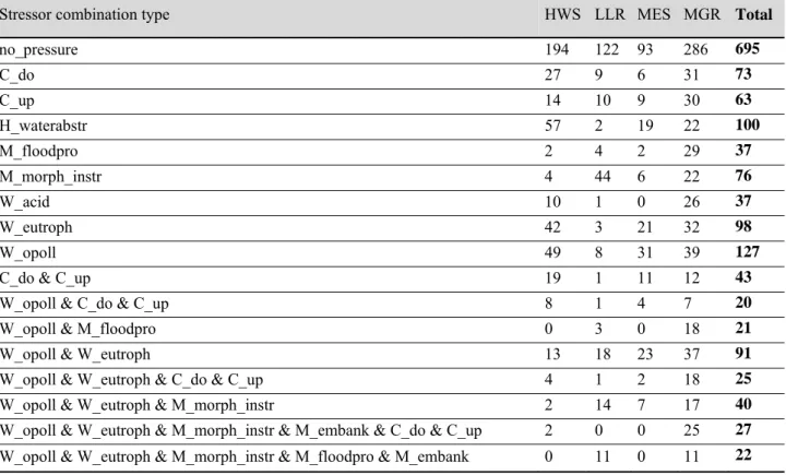
In terms of stressor distribution and frequent stressor combinations, we found eight single stressors (which affect 611 sites) and eight stressor combinations (which affect 1799 sites) and which are occurring frequently (at more than 20 sites of the overall dataset, in order to be representative for the following analyses). Moreover, 695 sites were unimpacted and thus are available as reference sites. The stressor distribution and frequent stressor combinations are shown in Table 3.
Table 4- Stressor distribution and frequent stressor combinations per Fish Assemblage Type
Stressor combination type HWS LLR MES MGR Total
no_pressure 194 122 93 286 695 C_do 27 9 6 31 73 C_up 14 10 9 30 63 H_waterabstr 57 2 19 22 100 M_floodpro 2 4 2 29 37 M_morph_instr 4 44 6 22 76 W_acid 10 1 0 26 37 W_eutroph 42 3 21 32 98 W_opoll 49 8 31 39 127
C_do & C_up 19 1 11 12 43
W_opoll & C_do & C_up 8 1 4 7 20
W_opoll & M_floodpro 0 3 0 18 21
W_opoll & W_eutroph 13 18 23 37 91
W_opoll & W_eutroph & C_do & C_up 4 1 2 18 25
W_opoll & W_eutroph & M_morph_instr 2 14 7 17 40
W_opoll & W_eutroph & M_morph_instr & M_embank & C_do & C_up 2 0 0 25 27
W_opoll & W_eutroph & M_morph_instr & M_floodpro & M_embank 0 11 0 11 22
Figure 8 shows the spatial location of unimpacted sites, sites impacted by single stressors and by stressor combinations.
Figure 8 - Location of fish sampling sites affected by single stressors (circle symbols) and combined stressors (triangle symbols).
Reaction of metrics to single stressors and stressor combinations
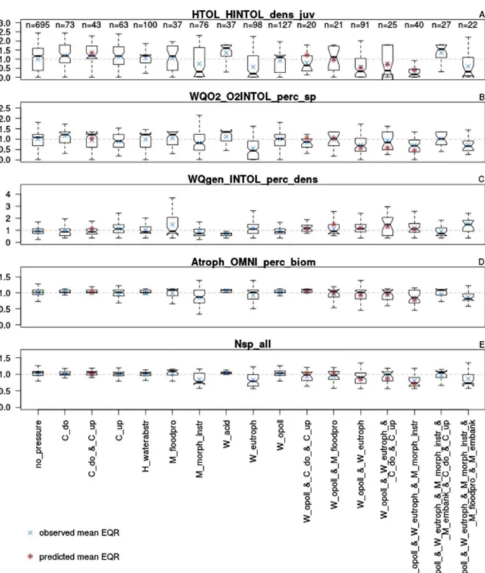
As shown by Figure 9 A-E, the five most important fish metrics in the random forest model also showed the best response to single stressors and stressor combinations in the boxplots.
These metrics were total abundance of juveniles (<150mm) intolerant to habitat degradation (HTOL_HINTOL_dens_juv, Figure 9 A), % of abundance of intolerant to general water quality
degradation (WQgen_INTOL_perc_dens, Figure 9 C), % of species intolerant to oxygen depletion
(WQO2_O2INTOL_perc_sp), % of omnivorous biomass (Atroph_OMNI_perc_biom, Figure 9 D) and total richness (Nsp_all, Figure 9 E). The strongest results where shown for two metrics: For
juveniles intolerant to habitat degradation, eutrophication as a single stressor and eutrophication in
combination with organic pollution and in-stream habitat degradation (Figure 9 A). For this case, the predicted combined stressor was lower than the observed joint interaction, which indicates a synergistic interaction.
Moreover, for % species intolerant to oxygen depletion, the strongest deviation was observed for eutrophication as a single stressor, and another strong synergistic interaction with organic pollution and in-stream habitat alteration (Figure 9 B).
Figure 9 A-E - Boxplots of the five most important fish metrics (displayed as EQR) and their reaction to single and multiple stressors (A – total abundance of juveniles intolerant to habitat degradation, B - % of species intolerant to oxygen depletion, C - % of abundance of intolerant to general water quality degradation, D - % of omnivorous biomass, E - total richness). The blue cross shows the observed mean EQR, the red asterisk the predicted mean EQR.
Multi-stressors analyses on lakes
Data and methodThe analyses were conducted on two datasets, one including the natural lakes of seven European countries and another on the Portuguese and French reservoirs.
Natural lakes - The fish data have been collected between 2003 and 2014 in the framework of the
intercalibration exercise, then updated during the WISER project. Natural lakes from Estonia, Denmark, France, Germany, Ireland, Norway and Sweden were used (Figure 10). Some French data were collected more recently at the occasion of new fish campaigns. All these lakes were sampled using the Norden gillnet standardised protocol (C.E.N., 2005). This method entails the use of pelagic and benthic nets. In this analysis, only fish data collected with benthic multi-mesh gillnets were used. These benthic nets were 30 m long and 1.5 m high, and composed of 12 different panels with mesh sizes ranging between 5 mm to 55 mm knot to knot in a geometric row. Random samplings were performed in different depth strata during the summer period. The number of nets set in each stratum depended on lake depth and area. A standard fishing period corresponded to one night (setting gillnets at dusk and lifting them at following dawn).
French and Portuguese reservoirs (Figure 11) - The French reservoirs were sampled following the
same method as natural lakes. Portuguese reservoirs were sampled between 2004 and 2005 using benthic multi-mesh nets measuring 30 x 2.5 m and composed of five panels of 6 m each with mesh sizes ranging from 30 to 95 mm knot to knot. The standard fishing period also covered sunset and sunrise periods and lasted 17 hours on average. As Portuguese reservoirs were sampled using different gillnets, the results of fishing campaigns had to be homogenised. We discarded captured fish individuals smaller than 90 mm and longer than 600 mm in French results to match with Portuguese size ranges.
In both European and South Western datasets, the fish caught were identified to species level, counted and weighed in grams. The fish catches were converted to catch per unit effort (number of fish/m² of net/night) and biomass per unit effort (g/m² of net/night).
Figure 11 – Distribution of the 236 French and Portuguese reservoirs.
Fish metrics
Traits used to describe species attributes were defined according to a literature survey elaborated from national experts’ judgment. Species were assigned to trophic guilds as follows: invertivorous (INV) species whose adult diet consists of more than 75% insects; planktivorous (PLAN) species whose adult diet consists of more than 75% zooplankton and/or phytoplankton; piscivorous species (PISC) feeding on fish, at least partly, as adults. Carnivorous (INV/PISC) species include individuals
that are both invertivorous and piscivorous. Species that are both invertivorous and planktivorous (INV_PLAN), invertivorous and herbivorous (INV_HERB), detritivorous and herbivorous (DETR_HERB) or benthivorous (BENT) were not abundant enough and these traits were not used. If plant and animal material both contributed at least 25% to the diet, the species was considered omnivorous (OMNI) (Schlosser, 1982). Species were also classified according to their pelagic (WC) or benthic (BENT) living and feeding habitats. The reproductive guilds considered were phytophilic (PHYT) species spawning on different parts of living or dead vegetation and lithophilic (LITH) species spawning on clean mineral substrate. Species showing indifferent spawning preferences were considered to be both phytophilic and lithophilic (PHLI). Reproductive traits represented by only a few species (ariadnophilic (ARIAD), and ostracophilic (OSTRA), i.e. species spawning in shells; pelagophilic (PELA) species spawning in the pelagic zone) were not taken into account. Species were also classified as being either tolerant (Tolerant) or intolerant (Intolerant) to any stressor related to lake morphology (habitat), hydrology or water chemistry (Karr et al., 1986). Finally, fish species were also sorted in reproductive behaviour guilds according to their guarding and nesting behaviour (Balon, 1981, 1975). The A guild includes non-guarders species, A_1_0 depositing eggs on open substrate while A_2_0 species hide their eggs. The B guild includes species guarding their eggs: B_1_0 species scatter them on plants and B_2_0 species construct nests. A_2_0 and B_1_0 were excluded as these traits were rarely represented in our datasets. All these metrics were expressed as the sum of the biomass and the sum of the abundances of the species they include. Total abundance and total biomass were included (ALL (CPUE) and ALL (BPUE)) and the ratio of roach (Rutilus
rutilus (L.)) to perch (Perca fluviatilis L.). Trait values for each species encountered in European and
South Western datasets are described in Appendix 1. It was decided to not integrate unknown species and hybrids in the calculation of metrics for functional guilds (Abramis sp., Coregonus sp., Cottus sp., Mugilidae unknown, Cyprinidae unknown) because the traits could be different from one species to another, even in the same family.
Thirty metrics were calculated using fifteen traits expressed as biomass (BPUE) or abundance (CPUE) of fish belonging to each guild. Similarly, total individuals and the ratio roach/perch was calculated in occurrence and biomass. A total of 34 metrics were used in the different analyses.
Environment and stressors
The variables given in Table 5 were included in the analyses. Maximum depth (Zmax) and Lake Area (LA) are strong drivers of fish species richness (Barbour and Brown, 1974; Eadie and Keast, 1984). Catchment area (ADB) can be considered as a surrogate for habitat diversity upstream from the lake (Irz et al., 2004).
Latitude and longitude were retained as biogeographical variables (decimal degree (WGS84)). Altitude (Alt) parameter can be related to isolation and climatic data (Godinho et al., 1998; Hinch et al., 1991; Magnuson et al., 1998). No mountain lakes above 1500 m were included because species richness is generally low; moreover, in these lakes, fish communities are generally strongly influenced by human introductions (Argillier et al., 2002a; Argillier et al., 2002b) and fish is not
considered as a relevant bioindicator to assess ecological status (Ministère de l'Ecologie et du Développement Durable, 2010).
January to December mean yearly air temperatures (TJanuary & TDecember) were obtained from the climate CRU model (New et al., 2002). January and July mean temperature allowed to derive the following independent variables related to temperature requirements of living organisms (Daufresne and Boet, 2007; Irz et al., 2007; Mason et al., 2008) :
(i) AveT = (TJanuary – TDecember)/12 (ii) AmpT = TJuly – TJanuary
Table 5 – Environmental variables in the European natural lakes and South-western reservoirs.
European dataset South-western subdataset
Mean Range Mean Range
Maximum depth (Zmax, m) 15.6 0.6 - 310 28.2 1.2 – 135
Lake Area (LA, km2) 2.3 0.01 – 577.1 3.3 0.01 – 577.1
Catchment Area (CA, km2) 82.1 0.05 – 10 628.9 30 001 0.7 – 963 000.0
Latitude (Lat, °) 57.9 43.6 – 69.7 45.9 37.3 – 50.9
Longitude (Long, °) 12.9 -10.2 – 30.8 1.5 -8.5 – 9.5
Altitude (Alt, m asl) 209.6 0 – 1 500 276.3 0 – 1 325.0
Mean temperature (AveT, °C) 5.3 -3.8 – 14.3 11.0 4.3 – 17.6 Temperature amplitude (AmpT, °C) 18.9 8.4 – 29.5 15.1 9.9 – 18.4
These parameters were also retained because of their availability (for example mean depth was excluded because of too many unknown values).
Altitude, maximum depth, lake area and catchment area were log-transformed for graphical display. A correlation between all natural parameters was performed to check their independence.
Environmental variables were grouped and summarized thanks to a PCA method. Groups were Biogeography (2 PCA axes), Climate (1 PCA axis) and Ecosytem size (2 PCA axes), respectively including latitude, longitude and altitude, mean temperature and temperature amplitude, and lake maximum depth, lake area and catchment area.
Stressors: Eutrophication was measured through Total Phosphorous mean annual concentrations.
This value was a mean of at least four measurements in a single year for all the lakes. Values were log-transformed to obtain a normal distribution. Non-native species presence was also taken into account as the proportion of non-native species in biomass. Non-native species status was assessed at the basin level thanks to the Fish SPRICH database (Brosse et al., 2013). Hydromorphological
stressors: In the work done at the European scale, for most of the lakes, the intensity of
(hydrological) and mostly morphological modifications were assessed by expert judgement and in some instances in application of the Lake Habitat Survey (Rowan et al., 2005). The lakes were then classified in two classes, one experiencing weak modifications and the other experiencing heavy modifications. In Portuguese and French reservoirs, alteration of the hydromorphology was always
measured in the framework of the Lake Habitat Survey. In these analyses, lakes were classified according to six stressor indices: shore zone modification, shore zone intensive use, in-lake use, hydrology, sediment regime and nuisance species (Rowan et al., 2005). Shore zone modification index measures the proportion of the shoreline affected by hard engineering. Shore zone intensive use measures the proportion of natural vs. artificial land cover on the shore line (Rowan et al., 2005). In-lake use quantifies the number of in-In-lake pressures such as dredging, macrophyte control, boat activities, angling, fish stocking etc. (Rowan et al., 2005). Nuisance index indicate the presence of terrestrial (i.e. the Japanese Knotweed Fallopia japonica) or aquatic (i.e. Nuttall’s pondweed Elodea
nuttallii) nuisance plants (Rowan et al., 2005). As hydrology index heavily penalizes dammed lakes
(i.e. the lowest note was attributed to all the reservoirs) and as in-lake use was not directly related to hydromorphology, we excluded these two indices from the analyses (Rowan et al., 2005).
Modelling
On the two datasets (Europeans lakes and South-western reservoirs), a random forest was grown for each fish metric. As previously described (section General approach), 2500 trees were grown per forest and, the percentage of explained variance and variables relative importance were computed (Breiman-Cutler permutation method). Random forest models were of the form fish metric ~ Biogeography + Ecosystem size + Climate + Eutrophication + Non-native species + Hydromorphological alterations.
We selected pertinent models by keeping only models in which at least one of the stressor variables explains 10% or more of the total variance.
In selected models, the intensity of interactions between stressors was assessed by computing the difference between their “Paired” importance and the sum of their individual importance (“Additive importance”) (Ishwaran, 2007). This difference value was expressed relatively to the “additive” importance. This process is described in details in the section “Pairwise approach – random forests”. Finally, for each of the selected models, we chose interactions of interests among all possible interactions, notably eutrophication × proportion of non-native species.
Finally, for both natural and artificial lakes, we analysed interactions involving the two stressor variables having the greatest relative importance. The only exception was in artificial lakes, the interaction between eutrophication and shore use for the abundance of B_2_0 species was also taken into account. Interactions were analysed and plotted thanks to co-plots representing the predicted response of fish metrics to a stressor variable (continuous or categorical) for different levels of another stressor variable (categorical).
Results
Effect of stressors on fish metrics of the European natural lakes
At the European level, models explained between 2.3 and 51.4% of the variance (Figure 12). The stressor variables explained at least 10% of the variance in eight models that where studied in details (Figure 12). Total explained variance of these models ranged from 28.2 to 39.5%.
Figure 12 - Total percentage of variance explained by stressor variables (in white) and the environment for each fish metric calculated with the abundance of fish (a) and the biomass of fish (b). The dashed line represents the threshold of variance explained above which the model was selected.
The eight metrics best explained by stressors were in relation with total occurrence (CPUE), tolerance, reproductive guilds (PHLI and A_1_0), trophic guild (OMNI and PLAN) and living and feeding habitats (BENT) (Figure 13). For most of these metrics, biogeography and size of the lakes explained the major part of the variability. However the proportion of non-native species and total phosphorus were the variables explaining most of the variability of the metric CPUE of planktivorous (relative VIMP of 21.1 and 20.3% respectively), and total phosphorus had a relative importance of 29.1% in the model explaining the BPUE of benthic species. Shore Bank Modification index showed only a poor relative importance and added little explanation power to the models (Figure 13). Indeed, in the selected metrics, the relative variable importance of SBM ranged from 0.002 to 0.9% while the relative variable importance of total phosphorus ranged from 15.2 to 29.1% and the relative variable importance of non-native species proportion was between 6 and 21.1%. In all cases, eutrophication was the stressor the more strongly related to fish metrics and the Shore Bank Modification index was systematically the least important variable.
ALL LITH PHLI PHYT INV OMNI PISC PLAN BENT WC A_1_0 Intolerant Tolerant INV_PISC B_2_0 Roach/Perch 0 10 20 30 40 50 0 10 20 30 40 50 a) Abundances (CPUE) % of explained variance ALL LITH PHLI PHYT INV OMNI PISC PLAN BENT WC A_1_0 Intolerant Tolerant INV_PISC B_2_0 Roach/Perch 0 10 20 30 40 0 10 20 30 40 b) Biomass (BPUE) % of explained variance
Figure 13 – Relative importance of environmental and stressor variables for the selected fish metrics. Biog1 & 2, size1 & 2 and clim1 are the PCA axes summarizing biogeography, ecosystem size and climate, respectively. Ltp and prop_nnb stand for the concentration of total phosphorus and the proportion of non-native species in biomass, respectively. SBM_class is a measure of Shore Bank Modification.
Interactions between stressors in European natural lakes
Differences and relative differences between Paired and Additive importance of stressor variables were weak (Figure 14). The greatest relative difference was -1.96% which indicates the very weak interactions between stressors studied on the fish European dataset we used. Co-plots indicated strictly additive interactions between eutrophication and the proportion of non-native species (Figure 15). A threshold effect of eutrophication seems to appear between first oligotrophic and then meso- and eutrophic lakes (Figure 15).
SBM_classsize1 prop_nnbclim1 ltp biog1 biog2 size2 Relative importance (%) 0 5 10 15 20
(a) Total abundance
SBM_classsize1 prop_nnbbiog1 clim1 size2ltp biog2 Relative importance (%) 0 5 10 15 20
(b) Phytolithophilic species (CPUE)
SBM_classsize1 clim1 biog1ltp prop_nnb biog2 size2 Relative importance (%) 0 5 10 15 20
(c) Omnivorous species (CPUE)
SBM_classsize1 biog1 prop_nnbclim1 biog2 ltp size2 Relative importance (%) 0 5 10 15 20 25
(d) Benthic species (CPUE)
SBM_classsize1 prop_nnbbiog1 clim1 size2 ltp biog2 Relative importance (%) 0 5 10 15 20
(e) A_1_0 species (CPUE)
SBM_classsize1 prop_nnbclim1 biog1 size2 ltp biog2 Relative importance (%) 0 5 10 15 20
(f) Tolerant species (CPUE)
SBM_classsize1 clim1 biog1 biog2 size2ltp prop_nnb Relative importance (%) 0 5 10 15 20
(g) Planktivorous species (CPUE)
SBM_classsize1 prop_nnbsize2 clim1 biog2 biog1ltp Relative importance (%) 0 5 10 15 20 25
Figure 14 - Paired and additive importance of stressor variables in European natural lakes. The difference between paired and additive values of variable importance measures the interaction between the variables. Interactions are ordered according to the difference value that is written above the bars and expressed relatively to the Additive importance. Positive values indicate synergistic interactions while negative values indicate antagonistic interactions.
Additive Paired V a ri a b le im p o rt a n c e 0.00 0.02 0.04 0.06 0.08 0.10 ltp:p rop_ nnb SBM _clas s:pr op_ nnb ltp:S BM _cla ss 0.89 % 0.83 % -0.05 %
(a) Total abundance
Additive Paired V a ri a b le im p o rt a n c e 0.00 0.02 0.04 0.06 0.08 0.10 ltp:p rop_ nnb SBM _clas s:pr op_ nnb ltp:S BM _cla ss 1.83 % 0.51 % 0.05 %
(b) Phytolithophilic species (cpue)
Additive Paired V a ri a b le im p o rt a n c e 0.00 0.01 0.02 0.03 0.04 ltp:pr op_ nnb SB M_cl ass: prop_n nb ltp: SBM _clas s 0.55 % 0.18 % 0.16 %
(c) Omnivorous species (cpue)
Additive Paired V a ri a b le im p o rt a n c e 0.000 0.002 0.004 0.006 0.008 ltp:pr op_ nnb SB M_c las s:pr op_n nb ltp: SBM _clas s -1.96 % 0.22 % -0.07 %
(d) Benthic species (cpue)
Additive Paired V a ri a b le im p o rt a n c e 0.00 0.02 0.04 0.06 0.08 0.10 0.12 ltp:pr op_ nnb SBM _clas s:pr op_n nb ltp:S BM _cla ss 1.87 % 0.88 % -0.03 %
(e) A_1_0 species (cpue)
Additive Paired V a ri a b le im p o rt a n c e 0.00 0.02 0.04 0.06 0.08 ltp:pr op_ nnb ltp:S BM _cla ss SBM _cla ss:pr op_nn b 1.12 % 0.44 % 0.41 %
(f) Tolerant species (cpue)
Additive Paired V a ri abl e i m por ta nc e 0 2 4 6 8 ltp:pr op_ nnb SB M_cl ass: prop_n nb ltp:S BM_ clas s -0.39 % 0.27 % 0.01 %
(g) Planktivorous species (bpue)
Additive Paired V a ri abl e i m por ta nc e 0 5 10 15 20 25 30 35 SB M_c lass :pro p_n nb ltp:S BM_ clas s ltp:pr op_n nb 0.54 % 0.22 % 0.09 %
Figure 15 - Partial relations of non-native species with selected fish metrics in different contexts of
eutrophication. Thresholds between oligotrophic, meso- and eutrophic groups were 20 and 45 µg L-1.
Effect of stressors of fish metrics in the French and Portuguese reservoirs
Regarding the French and Portuguese reservoirs, random forest models explained up to 55.3% of the variance of all the fish metrics calculated on the dataset, and stressors accounted a maximum of 32.0% of the explaining power (Figure 16). Nine fish metrics in which at least 10% of the variance was explained by stressor variables were selected. The total explained variance of these selected metrics ranged from 27.8 to 55.3% (Figure 16).
0.4 0.6 0.8 0.00 0.25 0.50 0.75 1.00 Proportion of non-native-species Tot a l abun danc e group oli mid eu 0.2 0.4 0.6 0.8 0.00 0.25 0.50 0.75 1.00 Proportion of non-native-species P h y tol it hoph il ic s pec ie s group oli mid eu 0.2 0.3 0.4 0.00 0.25 0.50 0.75 1.00 Proportion of non-native-species O m ni v o rous s pec ie s group oli mid eu 0.05 0.10 0.15 0.20 0.00 0.25 0.50 0.75 1.00 Proportion of non-native-species B ent hi c s pec ie s ( c pue) group oli mid eu 0.4 0.6 0.8 0.00 0.25 0.50 0.75 1.00 Proportion of non-native-species A _1_ 0 sp ec ie s group oli mid eu 0.2 0.4 0.6 0.8 0.00 0.25 0.50 0.75 1.00 Proportion of non-native-species T o le ra nt sp eci e s group oli mid eu
Figure 16 - Total percentage of variance explained by stressor variables (in white) and the environment for each fish metric calculated with the abundance of fish (a) and the biomass of fish (b). The dashed line represents the threshold of variance explained above which the model was selected.
The first result was that hydromorphological impacts were only weakly related to fish metrics compared to eutrophication and non-native species relative importance (Figure 17).
Again, biogeography and ecosystem size variables were important while climate was usually a minor environmental variable (maximum relative importance variable = 13.4% for the abundance of lithophilic species).
B_2_0 species abundance and biomass, and total biomass were clearly related to stressor variables.
The proportion of non-native species and eutrophication explained more variance than environmental variables. Planktivorous species, benthic species, tolerant species and A_1_0 species were also strongly related to eutrophication which was systematically the main or one of the main variables and had a relative importance > 20%. Lithophilic species were mainly explained by the proportion of non-native species (relative importance = 32.7%).
In the model explaining the biomass of tolerant species, the shore use intensity variable had a relative importance of 3% and was ranked 6th out of 11 (Figure 17). Except in that case, hydromorphological variables were systematically the four least important variables.
ALL LITH PHLI PHYT INV OMNI PISC PLAN BENT WC A_1_0 Intolerant Tolerant INV_PISC B_2_0 Roach/Perch 0 10 20 30 40 0 10 20 30 40 a) Abundances (CPUE) % of explained variance ALL LITH PHLI PHYT INV OMNI PISC PLAN BENT WC A_1_0 Intolerant Tolerant INV_PISC B_2_0 Roach/Perch 0 10 30 50 0 10 30 50 b) Biomass (BPUE) % of explained variance
Figure 17 - Relative importance of the environmental and stressor variables for each selected fish metric. Biog1 & 2, size1 & 2 and clim1 are the PCA axes summarizing biogeography, ecosystem size and climate, respectively. Ltp and prop_nnb stand for eutrophication and the proportion of non-native species in biomass, respectively. SBM_class is a measure of Shore Bank Modification.
Interactions between stressors in French and Portuguese reservoirs
The strength of interactions between stressor variables was assessed by computing the difference between additive and paired importance (Figure 18 ;
shoremod sediment shoreuse size2 nuisance ltp biog2 size1 clim1 prop_nnb biog1 Relative importance (%) 0 5 10 20 30
(a) Lithophilic species (cpue)
shoremod nuisance sediment biog1 size2 shoreuse clim1 ltp size1 biog2 prop_nnb Relative importance (%) 0 10 20 30 (b) B_2_0 species (cpue) prop_nnb shoremod nuisance sediment shoreuse clim1 biog1 size2 biog2 size1 ltp Relative importance (%) 0 10 20 30 (c) Total biomass shoremod nuisance sediment shoreuse prop_nnb size2 clim1 ltp biog1 size1 biog2 Relative importance (%) 0 5 10 15 20 (d) Phytolithophilic species (bpue) shoremod nuisance shoreuse sediment clim1 size2 biog1 prop_nnb biog2 ltp size1 Relative importance (%) 0 5 10 15 20 25 30
(e) Planktivorous species (bpue) shoremod shoreuse nuisance sediment prop_nnb size2 biog2 size1 clim1 biog1 ltp Relative importance (%) 0 5 10 20 30 (f) Benthic species (bpue) shoremod sediment nuisance prop_nnb clim1 shoreuse biog1 size2 ltp size1 biog2 Relative importance (%) 0 5 10 15 20 25 (g) Tolerant species (bpue) sediment shoremod shoreuse nuisance prop_nnb clim1 size2 size1 biog1 biog2 ltp Relative importance (%) 0 5 10 15 20 25 (h) A_1_0 species (bpue) shoremod sediment nuisance shoreuse biog1 clim1 size2 ltp size1 biog2 prop_nnb Relative importance (%) 0 10 20 30 40 50 (i) B_2_0 species (bpue)
Figure 19 ; Figure 20) and, similar to natural lakes, most of the time the differences were weak.
Although we observed some great relative differences (see Figure 18a shoremod:shoreuse and Figure 18b shoremod:nuisance), the variance explained by these stressors indicated only a poor significance of the interaction.
For metrics based on the fish occurrences (Figure 18), in the models explaining the abundance of
lithophilic species and of B_2_0 species (building a nest), eutrophication and the proportion of
non-native species had slightly different importance whether they were separated or paired (Figure 18ab ; Figure 19ab). The co-plot showed synergitic interactions of these stressors on the two metrics. In the model explaining the abundance of B_2_0 species (Figure 18b ; Figure 19c), the interaction between eutrophication and the intensity of shore use seems significant with a relative difference of -6.65% but the graphical analyses of the co-plot didn’t confirm a synergistic or antagonistic interaction (Figure 20).
Figure 18 - Paired and additive importance of stressor variables for metrics based on abundances in the French and Portuguese reservoirs. The difference between paired and additive values of variable importance measures the interaction between the variables. Interactions are ordered according to the difference value that is plotted above the bars and expressed relatively to the Additive importance.
Additive Paired 0.000 0.005 0.010 0.015 0.020 0.025 0.030 shor emod: shor eus e nui sanc e:sedi ment ltp: prop_nnb ltp:s hor eus e shor emod: sedi me nt shor euse :sedi ment shor em od: nui sanc e ltp: shor emod nui sanc e:pr op_nn b ltp: sedi ment ltp:nu isanc e shor em od: prop_nn b shor euse :prop_ nnb sedi me nt:pr op_nnb shor euse :nu isanc e -78.55%-10.97% -3.08% -2.78% -2.72% 2.36%-1.37%1.22% -0.75% -0.35% -0.3% 0.29% 0.16% 0.1% 0.03%
(a) Lithophilic species (cpue)
V a ri abl e i m por tanc e Additive Paired 0.000 0.005 0.010 0.015 0.020 0.025 shore mod: nui sanc e nui sanc e:sedi ment shor emod: sedi me nt ltp: shor eus e shor em od:s hor eus e ltp: prop_nnb shor euse :sedi ment shor em od: prop_nn b ltp:s edi ment ltp:s hor em od shor euse :nui sanc e shor euse :prop_ nnb ltp:nui sanc e sedi me nt:pr op_nnb nui sanc e:pr op_nn b -18.41%-13.09%-7.13% -6.65% -4.08% -3.54% -3.04% 1.27% 1.1% -1.09% -0.93% 0.9% -0.78% 0.63% -0.44% (b) B_2_0 species (cpue) V a ri abl e i m por tanc e
Figure 19 - Paired and additive importance of stressor variables for functional metrics based on biomass in the French and Portuguese reservoirs. The difference between paired and additive values of variable importance measures the interaction between the variables. Interactions are ordered according to the difference value that is plotted above the bars and expressed relatively to the Additive importance.
Additive Paired 0 100 200 300 400 500 shor em od:pr op_nn b shor euse :pro p_nn b sed imen t:pr op_n nb ltp: sedim ent sho reu se:se dim ent shor euse :nu isan ce shor em od:se dim ent shor em od:nu isa nce nui san ce:pr op_nn b ltp: shor emo d shor em od:sh oreu se ltp:sh oreu se nuis ance :se dim ent ltp:p rop_ nnb ltp:n uisa nce 6.99% 2.79% -2.37% -1.91% -1.79% 1.68%-1.47% 1.4% -1.36% -1% 0.94% -0.82% 0.64% -0.32% 0.07%
(a) Total biomass
V a ri a b le im p o rt a n c e Additive Paired 0 20 40 60 80 sedim ent :pro p_n nb shor em od:sh ore use shor em od:n uisa nce shore mod :sed imen t shor euse :pro p_nnb shor euse :nui sanc e ltp:s edim ent shor em od:pr op_n nb ltp:sh ore mod nuis anc e:s edim ent ltp:n uisa nce shor euse :sed iment ltp:s hor euse nuis ance :pro p_n nb ltp:p rop_n nb 3.38% -1.99% 1.71%-1.04% 1% 0.98% -0.56% -0.48% 0.48% -0.42% 0.35% 0.31% -0.18% 0.15% 0.03%
(b) Planktivorous species (bpue)
V a ri ab le im p o rt an c e Additive Paired 0 50 100 150 200 250 300 350 sedim ent:p rop_ nnb shor euse :nu isa nce shor em od:s edim ent shor em od:s hore use shor eus e:s edim ent ltp:s edim ent nuis ance :sed iment nuis ance :prop_n nb ltp:p rop_ nnb ltp: nuis anc e shore use :prop _nnb ltp:s hore use shor em od:p rop_n nb shor em od:n uisanc e ltp:s hore mod 5.45% 3.15%-2.38%-2.19%-2.07% -1.78% -1.58%-1.47% -1.2% -0.51% 0.22% -0.2% 0.13%-0.05% -0.05%
(c) Benthic species (bpue)
Va ri a b le im p o rt a n c e Additive Paired 0 50 100 150 200 250 300 shore mod :se dim ent nuis ance: sedim ent shor euse :pro p_nnb ltp:p rop_ nnb sedi men t:prop_ nnb nui sance :prop _nnb shor eus e:n uisan ce shore mod :prop _nnb ltp:s hore mod ltp: sedi men t shor euse :sed iment ltp:n uisa nce shor em od:n uisa nce ltp: shor eus e shor em od:s hor eus e -2.62%-2.43% 2.07% -2% -1.57% 1.38%-1.02%-0.64% -0.64% -0.5% -0.42% 0.21% -0.13% 0.12% 0.02%
(d) Tolerant species (bpue)
V a ri a b le im p o rt a n c e
Figure 20 - Paired and additive importance of stressor variables for reproductive trait metrics based on biomass in the French and Portuguese reservoirs. The difference between paired and additive values of variable importance measures the interaction between the variables. Interactions are ordered according to the difference value that is plotted above the bars and expressed relatively to the Additive importance.
In the models testing fish metrics biomass, interactions were globally weaker than for models testing fish metric abundance (Figure 21 and Figure 22). In many cases, interactions between eutrophication and the proportion of non-native species were selected due to their great importance compared to hydromorphological alteration variables (Figure 17). For total biomass and biomass of tolerant
species, the interaction between eutrophication and shore use was selected.
Additive effects of stressors were most frequently observed for the selected metrics (Figure 22). Slight synergistic effects between eutrophication and the abundance of non-native species was observed on the biomass of tolerant species. A clear synergetic effect was also observed between
Additive Paired 0 50 100 150 200 nui sanc e:sedi ment shor emod:n uisan ce shor em od: shor eus e sedi men t:pr op_nnb ltp:s hor eus e shor euse :sedi ment ltp: prop _nnb shor emod: sedi me nt ltp:s edi ment shor euse :nui sanc e shor euse :prop_ nnb shor em od: prop_nn b ltp:s hor em od nui sanc e:pr op_nn b ltp:nu isanc e -3.2% 1.01% -0.68%0.64% 0.63% -0.58% 0.57% -0.55% 0.53% -0.45%0.39% -0.26% 0.08% 0.08% -0.04%
(a) Phyto-lithophilic species (bpue)
V a ri abl e i m por tanc e Additive Paired 0 50 100 150 200 250 300 nui sanc e:sedi ment shor euse :sedi ment sedi me nt:pr op_nnb ltp: shor em od ltp: prop_nnb shor euse :prop_ nnb shor em od: prop_nn b shor emod:s hor eus e shor euse:n uisanc e ltp: shor eus e ltp:s edi ment shor em od:nui sanc e shor em od: sedi me nt ltp:nui sanc e nui sanc e:pr op_nn b -3.67%-3.21% 2.73% -2.65%-1.51% 1.29% 1.09% 1.04% 1.02% -0.79%-0.78% 0.18%-0.17% 0.07% 0.07%
(b) A_1_0 species (bpue)
V a ri abl e i m por tanc e Additive Paired 0 20 40 60 80 100 120 140 shor em od: sedi ment nui sanc e:sedi ment shor em od: nuis ance shor em od:s hor eus e shor euse :sedi ment ltp: prop_nnb shor euse :nui sanc e ltp: shor eus e shor euse :prop_ nnb ltp: sedi ment sedi men t:pr op_nnb shor em od:pr op_nn b ltp:shor em od ltp:nui sanc e nui sanc e:pr op_nn b 48.22% 35% -20.26%-17.22%6.98% -4% 3.88%-2.94% 0.7% -0.66% 0.47% 0.38% 0.33%-0.22% -0.2% (c) B_2_0 species (bpue) V a ri abl e i m por tanc e
![Figure 1 - Spatial location of sites [n = 3105] and associated fish assemblage type (FAT’s according to Schinegger et al., 2013)](https://thumb-eu.123doks.com/thumbv2/123doknet/14760628.584923/11.892.194.682.186.796/figure-spatial-location-sites-associated-assemblage-according-schinegger.webp)