Satellite measurements of the global mesospheric sodium layer

(1)

HAL Id: hal-00302724

https://hal.archives-ouvertes.fr/hal-00302724

Submitted on 25 Apr 2007

HAL is a multi-disciplinary open access

archive for the deposit and dissemination of sci-entific research documents, whether they are pub-lished or not. The documents may come from teaching and research institutions in France or abroad, or from public or private research centers.

L’archive ouverte pluridisciplinaire HAL, est destinée au dépôt et à la diffusion de documents scientifiques de niveau recherche, publiés ou non, émanant des établissements d’enseignement et de recherche français ou étrangers, des laboratoires publics ou privés.

Satellite measurements of the global mesospheric sodium

layer

Z. Y. Fan, J. M. C. Plane, J. Gumbel, J. Stegman, E. J. Llewellyn

To cite this version:

Z. Y. Fan, J. M. C. Plane, J. Gumbel, J. Stegman, E. J. Llewellyn. Satellite measurements of the global mesospheric sodium layer. Atmospheric Chemistry and Physics Discussions, European Geosciences Union, 2007, 7 (2), pp.5413-5437. �hal-00302724�

(2)

ACPD

7, 5413–5437, 2007 Global Na layer Z. Y. Fan et al. Title Page Abstract Introduction Conclusions References Tables Figures ◭ ◮ ◭ ◮ Back Close

Full Screen / Esc

Printer-friendly Version Interactive Discussion

EGU Atmos. Chem. Phys. Discuss., 7, 5413–5437, 2007

www.atmos-chem-phys-discuss.net/7/5413/2007/ © Author(s) 2007. This work is licensed

under a Creative Commons License.

Atmospheric Chemistry and Physics Discussions

Satellite measurements of the global

mesospheric sodium layer

Z. Y. Fan1, J. M. C. Plane2, J. Gumbel3, J. Stegman3, and E. J. Llewellyn4 1

School of Environmental Sciences, University of East Anglia, Norwich NR4 7TJ, UK

2

School of Chemistry, University of Leeds, Leeds, LS2 9JT, UK

3

Department of Meteorology, Stockholm University, 10691 Stockholm, Sweden

4

ISAS, Department of Physics and Engineering Physics, University of Saskatchewan, Saskatoon, SK S7N 5E2, Canada

Received: 29 March 2007 – Accepted: 7 April 2007 – Published: 25 April 2007 Correspondence to: J. M. C. Plane (j.m.c.plane@leeds.ac.uk)

(3)

ACPD

Full Screen / Esc

EGU

Abstract

Optimal estimation theory is used to retrieve the absolute Na density profiles in the mesosphere/lower thermosphere from limb-scanning measurements of the Na radi-ance at 589 nm in the dayglow. Two years of observations (2003 and 2004), recorded by the OSIRIS spectrometer on the Odin satellite, have been analysed to yield the

sea-5

sonal and latitudinal variation of the Na layer column abundance, peak height, and peak width. The layer shows little seasonal variation at low latitudes, but the winter/summer ratio increases from a factor of ∼3 at mid-latitudes to ∼10 in the polar regions. Com-parison of the measurements made at about 06:00 and 18:00 LT shows little diurnal variation in the layer, apart from the equatorial region where, during the equinoxes,

10

there is a two-fold increase in Na density below 94 km between morning and evening. This is most likely caused by the strong downward wind produced by the diurnal tide between ∼02:00 and 10:00 LT. The dramatic removal of Na below 85 km at latitudes above 50◦_{during summer is explained by the uptake of sodium species on the ice} sur-faces of polar mesospheric clouds, which were simultaneously observed by the Odin

15

satellite.

1 Introduction

Meteoric ablation is the source of the layer of neutral sodium atoms that occurs globally in the upper mesosphere/lower thermosphere (MLT) between 80 and 105 km (Plane, 2003). The Na layer was discovered nearly 80 years ago: radiation at 589 nm was

20

observed in the night sky spectrum (Slipher, 1929), and later identified as emission from neutral sodium atoms within the atmosphere (Bernard, 1939). In the 1950s, the layer was observed from resonance fluorescence at 589 nm (Na(32P_J – 32S₁_/2)) during twilight (Hunten, 1967). The variation of the fluorescence signal as the solar termina-tor passed through the layer enabled the layer profile to be determined. The

abso-25

(4)

ACPD

Full Screen / Esc

EGU measured Na resonant scattering signal (Hunten, 1954; Chamberlain, 1956; Hunten,

1967).

Measurements of the Na D-line emission in the dayglow were then performed using a Zeeman photometer, which utilized an oscillating magnetic field around a sodium vapour cell to filter out the NaD-line spectrum and hence discriminate against

5

Rayleigh-scattered sunlight (Blamont and Donahue, 1961). The Na layer was also studied during the day by ground-based photometric measurements of atomic Na ab-sorption (Chamberlain, 1956), and by rocket-borne photometric measurements of the dayglow (Donahue and Meier, 1967). However, because of the passive mode of pho-tometric measurements, where solar radiation is the only excitation source, the

obser-10

vations were confined to the twilight or dayglow.

The invention of the tunable laser enabled enormous progress to be made with the development of the lidar (light detection and ranging) technique in the late 1960s (Bow-man et al., 1969). Lidar provided (Bow-many advantages over photometers. Firstly, by active excitation of the atmospheric Na, observations could be performed over a full

diur-15

nal cycle: initially, night-time measurements were performed (Gibson and Sandford, 1971), but modified receivers to exclude scattered sunlight then enabled daytime mea-surements to be made (Gibson and Sandford, 1972). These meamea-surements quickly showed that the apparent enhancement of the Na layer during daytime, reported from photometric measurements of the dayglow (Blamont and Donahue, 1961), was not

20

correct. Long-term observations of the Na layer provided more details of seasonal, lat-itudinal and diurnal variations (e.g. Megie and Blamont, 1977; Clemesha et al., 1979; Kirchhoff and Clemesha, 1983; Gardner et al., 1988; Tilgner and von Zahn, 1988; von Zahn, et al., 1988; Plane et al., 1999; She et al., 2000; Clemesha et al., 2004; Gardner et al., 2005).

25

Of course, an important limitation with lidar measurements is that the instruments are usually ground-based, and thus provide only localized coverage (airborne lidars partially overcome this difficulty (Kane et al., 1991; Plane et al., 1998a), but only for short campaigns). Global coverage can only be provided by space-borne instruments.

(5)

ACPD

Full Screen / Esc

EGU In fact, the first satellite-borne observations of the sodium nightglow were made two

decades ago (Newman, 1988), although the conclusions of that study were subse-quently criticized (Clemesha et al., 1990). The Na nightglow is generated from a chemi-lumiscent cycle involving Na, O3and O (Chapman, 1939), and so the complication of using nightglow observations is that the Na atom density is derived indirectly (Xu et al.,

5

2005). Recently, Fussen et al. reported global measurements of the mesospheric Na layer by the GOMOS stellar occultation instrument (i.e., the Na density was measured by atomic absorption) on the ENVISAT satellite (Fussen et al., 2004). Unfortunately, as we will discuss below, the retrieved Na column abundances, layer density profiles, and the seasonal and latitudinal variations are in poor agreement with the available data

10

from ground-based lidars.

We have recently developed a new method (Gumbel et al., 2007) using optimal esti-mation theory (Rodgers, 2000) to retrieve the absolute mesospheric Na density profile from limb-scanning satellite observations of the NaD-lines in the dayglow. The method has been validated by comparing Na profiles, retrieved from the OSIRIS spectrometer

15

on the Odin satellite, with profiles measured during overflights of the Na lidar at Ft. Collins, Colorado. The details of the methodology and error characterization are con-tained in our earlier paper (Gumbel et al., 2007). OSIRIS measures irradiance in the limb at wavelengths between 280 and 800 nm, with a resolution of ∼1 nm (Llewellyn et al., 2004). Odin is in a Sun-synchronous orbit at a height of ∼600 km, with an

ascend-20

ing node at ∼18:00 h local time (LT) and descending node at ∼06:00 LT (Murtagh et al., 2002).

In this paper, we have used this method to analyse two years of Odin data (2003 to 2004), in order to obtain the global seasonal distribution of the Na layer. During these two years there was a high frequency of mesospheric measurements in July/August,

25

because during these northern hemisphere summer periods Odin was dedicated to observing polar mesospheric clouds (PMCs) by limb-scanning between 70 and 110 km.

(6)

ACPD

Full Screen / Esc

EGU

2 Global Latitudinal and Seasonal Variations

Figure 1 illustrates the global coverage of the retrieved Na total abundance or column density (in units of Na atom cm−2), where the retrieved Na density profiles have been in-tegrated from 70 to 120 km. The data is zonally averaged to increase the data available in some latitude bins. In order to avoid artefactual distortions introduced by contouring

5

the data, this map is plotted in a grid format, with each grid box corresponding to 10◦ in latitude. The number inside each grid box indicates the number of integrated Na density profiles that have been averaged to produce the resulting column density. The blank grid boxes show occasions when mesospheric dayglow measurements could not be made because the solar zenith angle was larger than 92◦_{. This occurred in the}

win-10

ter hemisphere at mid- to high latitudes. The blank grid boxes at very high latitudes (>85◦_{) occur because of these regions are not covered by the satellite orbits.}

As many previous ground measurements have reported, the Na layer exhibits sea-sonal variations at all latitudes higher than 20◦: the total Na column density decreases to a minimum near the summer solstice and reaches a maximum in early winter. During

15

mid-summer and the whole winter period, the Na abundance exhibits relatively small fluctuations compared with the much greater variability during the spring and autumn equinoxes. Figure 1 shows that the seasonal variation from summer minimum to win-ter maximum becomes larger at higher latitudes. Although the data from mid-winwin-ter months is absent (except at low latitudes), we can still estimate the seasonal ratio by

20

employing the available data from late autumn/early winter. The data in Fig. 1 is in good accord with ground-based measurements at ∼40◦_{N (Megie and Blamont, 1977; Plane} et al., 1999; States and Gardner, 1999; She et al., 2000), at 51◦N (Gibson and Sand-ford, 1971), at 23◦S (Clemesha et al., 1979), at 43◦S (Hunten et al., 1964), and at 90◦S (Gardner et al., 2005). The maximum Na layer density usually occurs in about October

25

in the northern hemisphere (NH), and in about April in the southern hemisphere (SH). At low latitudes, this ratio is ∼2, and rises to ∼3 at middle latitudes. In polar region, this ratio increases up to nearly 10. The minimum monthly averaged Na abundance in

(7)

ACPD

Full Screen / Esc

EGU Fig. 1 occurs in July at 80◦_{N, and the maximum is during October at 80}◦_{N. In the}

equa-torial region (±10◦), by contrast, the seasonal variations are very small: the seasonal transitions between northern and southern hemisphere merge here, with a minimum in about March/April and a maximum in January/February. The seasonal ratio is typically no more than 1.5.

5

In order to understand the seasonal variation and latitudinal distribution of the Na abundance, we need to consider mesospheric sodium chemistry. In the mesosphere and lower thermosphere (MLT), Na+ ions and sodium bicarbonate (NaHCO3) are the major reservoir species above and below the atomic Na layer, respectively (Plane et al., 1999; Plane, 2004). Due to the long residence time of ablated sodium in the region

10

between 80 and 100 km (∼7 days) (Plane, 2004), and the comparatively short lifetimes of the rate-determining chemical reactions that convert sodium between atomic Na and these reservoirs, the chemistry reaches a photochemical steady-state on the timescale of vertical transport by eddy or molecular diffusion (Plane et al., 1998b). Consequently, atmospheric chemistry plays a key role in determining the atomic Na distribution. Na

15

is converted to NaHCO₃via the following sequence of reactions (Plane, 2004):

Na + O3→ NaO + O2 (1)

NaO + H2O → NaOH + OH (2)

NaOH + CO2(+M) → NaHCO3(M=N2orO2) (3)

All of these reactions are fast, with small temperature dependences. NaHCO3 is

con-20

verted back to Na by the reaction:

NaHCO₃+ H → Na + H2CO3 (4)

In contrast, this reaction has a large activation energy (Cox et al., 2001); that is, at higher temperatures it becomes much faster, and the steady-state balance shifts from NaHCO3to Na. A secondary effect is that O3 forms from the recombination of O and

25

(8)

ACPD

Full Screen / Esc

EGU concentrations slow down the conversion of Na to NaO, and the larger O concentrations

reduce NaO back to Na, enhancing the effect of Reaction (4) becoming faster.

At high latitudes, several factors further reinforce the positive temperature depen-dence of the Na density below 96 km. The first of these is the removal of sodium species on the ice surfaces of PMCs, which form between 82 and 85 km during

sum-5

mer at high latitudes when the temperature decreases below ∼150 K (Gardner et al., 2005; Murray and Plane, 2005; She et al., 2006). These low temperatures are caused by upwelling air (via adiabatic expansion) which also transports H2O from the lower mesosphere to above 80 km (Livesey et al., 2003), thereby increasing the rate at which Na is converted to NaHCO₃ (Reaction 2). Conversely, during winter there is strong

10

downward transport by the meridional wind (Portnyagin et al., 2004; Gardner et al., 2005), which has two effects: the temperature increases because of adiabatic heating, and Na is transported downwards from the peak of the layer.

Figure 2 illustrates the latitudinal distribution of the correlation coefficient between the retrieved Na density and temperature (taken from the MSIS model, Picone et al.,

15

2002), as a function of height. At middle and high latitudes, a strong positive correlation between temperature and Na density is seen below 96 km. This correlation is expected in view of the effects of temperature on the neutral sodium chemistry (see above), and has also been seen in mid-latitude lidar data (Plane et al., 1999).

At altitudes above 96 km, the correlation coefficient abruptly turns negative. This is

20

because ion chemistry dominates on the topside of the Na layer. Na+ions are formed by charge transfer with ambient NO+ and O+₂ ions and, to a lesser extent, by photo-ionization (Plane, 2004). These processes are essentially temperature-independent. In contrast, the neutralization of Na+ begins by forming a cluster ion with N2:

Na++ N2(+M) → Na+.N2, where M=N2or O2 (5)

25

This cluster ion can switch with more stable ligands such as CO2 or H2O, or be re-duced back to Na+ by atomic O, which slows the overall process (Cox and Plane, 1998). However, the cluster ions eventually undergo dissociative electron recombina-tion to yield Na. Reacrecombina-tion (5) is an associarecombina-tion reacrecombina-tion with a negative temperature

(9)

ACPD

Full Screen / Esc

EGU dependence (Cox and Plane, 1998): that is, at lower temperatures the cluster ions form

more rapidly, and so the steady-state balance between Na+ and Na shifts towards the neutral atom.

At low latitudes (± 20◦), the Na density does not exhibit a consistently strong correla-tion with temperature either below or above 96 km. In contrast, there is a strong diurnal

5

variation in this region which appears to be driven by the diurnal tide (see below). Figure 3 illustrates the seasonal variability of the Na layer: the top panel shows the monthly Na profiles, zonally averaged in four latitude bands. The corresponding monthly temperature profiles are shown in the bottom panel. Once again, the positive correlation between Na and temperature below 96 km, and the anti-correlation above

10

this altitude, is clearly visible at latitudes higher than 20◦_{N and S. Figure 3a shows the} seasonal variation of the Na density in the Arctic (70◦N). Note the removal of Na on both the top and bottom of the layer during summer, which is much more pronounced than at lower latitudes. As discussed above, the removal on the bottom side is caused by the stability of the chemical reservoir NaHCO3at lower temperatures. However, this

15

is greatly amplified by the uptake of sodium species on PMC ice particles (discussed in more detail below). Because of vertical mixing, Na is also removed on the topside of the layer. The seasonal temperature variation becomes smaller at mid- and low latitudes, leading to less removal of Na during summer.

Figure 3(b) shows the Na profile at 40◦_{N. This latitude was chosen for direct}

com-20

parison with the Na layer seasonal dependence at 40◦N reported recently from stellar occultation measurements made by the GOMOS instrument on ENVISAT (Fig. 5 in Fussen et al., 2004). There are several major discrepancies with the results of the present study. First, the GOMOS retrievals show a second peak in the Na density dur-ing mid-summer, whereas the OSIRIS result is a mid-summer minimum, in accord with

25

the lidar observations of the night-time Na layer at Ft. Collins (Colorado) (She et al., 2000) and Urbana (Illinois) (Plane et al., 1999; States and Gardner, 1999). Second, the maximum Na density in the GOMOS retrievals is ∼2500 cm−3in March, compared with just over 5000 cm−3 _{during October/November for OSIRIS and the mid-latitude lidar}

(10)

ACPD

Full Screen / Esc

EGU observations. Third, the width of the Na layer retrieved by GOMOS at 40◦_{N is highly}

variable: it is narrowest in March (extending from 85–105 km), when the Na density at the layer peak is largest, and is much broader (75–110 km) in late summer when the peak density is a minimum. In contrast, Fig. 3b shows that the layer thickness re-trieved by OSIRIS at 40◦N is fairly constant, with the layer being somewhat broader in

5

early winter when the peak density is a maximum (again in good accord with the lidar observations).

The reasons for these very marked discrepancies between the results from OSIRIS and GOMOS are not clear. Although the GOMOS results are for 2003, and the OSIRIS results combine data from 2003 and 2004, there are no significant differences in the

10

OSIRIS Na layer data between these successive years. The OSIRIS measurements were made at 06:00 or 18:00 LT, whereas most of the GOMOS measurements were at around 09:00 or 23:00 LT. This might indicate that some diurnal effect could be responsible for the differences. Indeed, a limited number of GOMOS measurements were made over the whole range of LT, from which the diurnal behaviour of the Na

15

layer could be examined (Fussen et al., 2004). The data showed very little change in the layer at 06:00, 12:00 and 18:00 LT, and then a large decrease, by ∼40% between 70 and 90 km, at 24:00 LT. Strangely, such diurnal behaviour has not been observed by lidars located over a range of latitudes (Gibson and Sandford, 1972; Kirchhoff and Clemesha, 1983; States and Gardner, 1999; She et al., 2000). In conclusion, the

20

GOMOS results are not in accord with either the OSIRIS measurements or ground-based lidars, but it is unclear why this is the case.

Figure 4 illustrates the distribution of the full width at half maximum (FWHM) and peak height of the Na layer, as a function of latitude and month. Due to the limited vertical resolution in the retrieved profiles, these parameters cannot be determined

25

with the precision of a ground-based lidar. Nevertheless, useful results are obtained. Unsurprisingly, the FWHM is a minimum in polar summer, because of removal of Na on both the top and bottom of the layer (see above), whereas in winter the FWHM more than doubles at mid- to high latitudes. The peak height of the Na layer lies mostly

(11)

ACPD

Full Screen / Esc

EGU between 90 and 92 km. However, it is often higher (∼94 km) in the equatorial region,

as a result of the strong diurnal tide (see below).

3 Diurnal variation in the equatorial region

The Odin satellite takes measurements at about 06:00 LT (descending node) and 18:00 LT (ascending node), and the above analyses of seasonal properties of the

5

Na layer combine the morning and evening observations. Indeed, at mid- and high latitudes there is no significant diurnal difference. In contrast, a marked difference be-tween the morning and evening profiles is observed in the tropics, especially at the equinoxes. This is illustrated in Figs. 5a and b, which show the zonally averaged morn-ing and evenmorn-ing profiles, respectively, and Fig. 5c, which shows the difference between

10

the evening and morning, as a function of latitude. The Na layer in the tropical region (15◦N–30◦S) is strongly depleted in the morning. Most of the depletion occurs below 95 km, peaking at 88 km, and the morning layer column density is about 50% that in the evening.

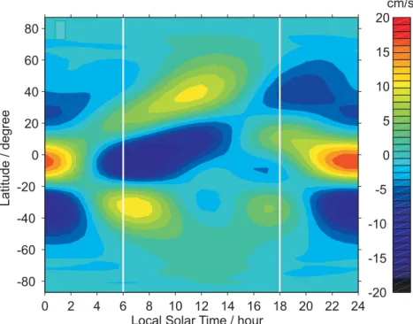
Figure 6 shows the latitudinal dependence of the vertical tidal wind velocity at an

15

altitude of 90.6 km (close to the peak of the Na layer), as a function of local time. This is calculated from the Global Scale Wave Model (GSWM) (Hagan and Forbes, 2002). Note that the largest wind velocities are in the tropical region (20◦N–20◦S). The strong downward wind, which actually starts around 100 km at midnight, appears at 91 km around 04:00 LT, reaches a miximum of –20 cm s−1 _{around 07:00 LT, and}

20

then dissipates after 10:00 LT. Between 14:00 LT and 18:00 LT, when the evening Odin measurements were made, the vertical wind reverses but its velocity is small, between –5 and +5 cm s−1_.

This tidal behaviour in the tropics should affect the Na layer in several ways which explain the diurnal behaviour of the tropical layer (Fig. 5). First, the strong downward

25

wind starting at midnight will cause a vertical displacement of 3–4 km by the time of the Odin measurement at 06:00 LT. Atomic Na, close to the layer peak at 91 km, will be

(12)

ACPD

Full Screen / Esc

EGU displaced into a region of higher pressure where the termolecular reaction

Na + O2(+M) → NaO2 (6)

will form sodium superoxide, a reasonably stable reservoir species (Plane, 2004). Re-action (3), which is pressure-dependent, will also increase and produce the more stable reservoir NaHCO₃.

5

The strong downward tidal wind also affects the constituents O and H. For example, during September the atomic O concentration derived from the Wind Imaging Inter-ferometer (WINDII) on the Upper Atmosphere Research Satellite exhibits a dramatic decrease (by over 50%) in the equatorial region between 02:00 LT and dawn, at alti-tudes up to about 95 km (Russell et al., 2005). Atomic O and H exert a major control

10

on the sodium chemistry through Reaction (4) and the reactions:

NaO2+ O → NaO + O2 (7)

NaO + O → Na + O2 (8)

The resulting decrease in the rates of Reactions (4), (7) and (8) then reinforce the conversion of Na to NaO₂and NaHCO₃, causing the observed depletion of Na atoms

15

at 06:00 LT (Fig. 5).

4 Polar Depletion of the Na Layer

The global minimum of the Na column abundance occurs at high latitudes during sum-mer, and can be an order of magnitude lower than the maximum (Fig. 1). At the same time, the FWHM width of the Na layer in the summertime polar region is also a

mini-20

mum (Fig. 4a), about half the width of the layer during winter or at lower latitudes. In this section the reasons for this extreme seasonal behavior in the polar regions will be discussed in more detail.

(13)

ACPD

Full Screen / Esc

EGU Figure 7 displays the sodium density profiles at mid- and high latitudes between

March and September, straddling the NH summer solstice. A white horizontal line has been drawn on each of the plots at 80 km to aid the eye in observing changes to the underside of the Na layer. Figure 8 compares the monthly variation of the mean Na layer profiles at latitudes of 40◦_{N and 80}◦_{N, from spring equinox to the summer}

5

solstice. The undersides of the Na profiles during the solstice show a clear cutoff below 85 km.

Previous ground-based lidar measurements have observed the very low minimum Na abundance in the Arctic region during summer (e.g. Gardner et al., 1988; von Zahn et al., 1988; Gardner et al., 2005). Recent research has focused on the

re-10

moval of metal atoms (and their compounds) on the surfaces of ice particles (Lubken and Hoffner, 2004; Plane et al., 2004), following a laboratory study which demonstrated that Fe, Na and K atoms are all removed very efficiently on low-temperature ice sur-faces (Murray and Plane, 2005). Simultaneous measurements of mesospheric Na, PMCs and polar mesosphere summer echoes (PMSE) (She et al., 2006) also found

15

that polar Na depletion is highly correlated with PMCs, whereas the smaller-sized ice particles detected by radar as PMSE exhibit a weaker anti-correlation with the Na den-sity around 85 km.

The satellite retrievals enable the full process of polar Na layer depletion to be tracked. In April and May, the Na layer shifts gradually to a summertime profile, mainly

20

due to the temperature-dependent Na chemistry discussed above, where a larger frac-tion of the sodium is in the form of NaHCO3. In June, July and August the underside of the Na layer exhibits a sharp cut-off at about 85 km. In the June and July profiles, the lower edge of the layer gradually rises northwards from ∼50◦N. The Na depletion on the underside disappears abruptly in September.

25

In a very recent paper (Petelina et al., 2006), the occurrence of PMC was derived from the same OSIRIS spectra that we have used to retrieve the Na density profiles. The results can therefore be used to explore the relationship between them. Although it is difficult to determine precisely the altitude of a PMC when viewed in the limb, the

(14)

ACPD

Full Screen / Esc

EGU PMC peak heights were found to be located mostly between 83–84 km (Petelina et al.,

2006). PMCs were observed from 50◦N to higher latitudes, and from the beginning of June until the end of August. The clouds appeared most frequently immediately after the summer solstice (Petelina et al., 2006). These PMC statistics are in complete accord with the polar Na profiles: the underside of the Na layer below 85 km disappears

5

completely from June until the end of August. In fact, since the bottom of the Na layer in polar regions is very sensitive to the presence of PMCs, it may be useful as an indicator of the presence of PMCs which are not optically detectable.

5 Conclusions

This paper demonstrates the ability of our new algorithm (Gumbel et al., 2007), based

10

on optimal estimation theory (Rodgers, 2000), to retrieve absolute Na density profiles from limb-scanning measurements of the NaD-line radiance at 589 nm in the dayglow. These global measurements provide a very useful complement to ground-based lidar observations. Particular highlights of the present data set are the first observations of the Na layer in the equatorial region. We find that the layer exhibits little seasonal

15

variability, but has a very marked diurnal variation, particularly during the equinoxes. This is almost certainly driven by the diurnal tide. The measurements in the polar regions confirm the relationship between depletion of Na below 85 km and the presence of PMCs during the summer at latitudes above 50◦.

Acknowledgements. Z. Y. Fan acknowledges contributions from the Universities of East Anglia, 20

Stockholm and Saskatoon towards his PhD studentship.

References

Bernard, R.: The Identification and the Origin of Atmospheric Sodium, Z. Phys., 110, 291–135, 1938.

(15)

ACPD

Full Screen / Esc

EGU

Blamont, J. E. and Donahue, T. M.: The Dayglow of the Sodium D Lines, J. Geophys. Res., 66, 1407–1427, 1961.

Bowman, M. R., Gibson, A. J., and Sandford, M. C.: Atmospheric Sodium Measured by a Tuned Laser Radar, Nature, 221, 456–458, 1969.

Chamberlain, J. W.: Resonance Scattering by Atmospheric Sodium. 1. Theory of the Intensity

5

Plateau in the Twilight Airglow, J. Atmos. Terr. Phys., 9, 73–89, 1956.

Chapman, S.: Notes on atmospheric sodium, J. Astrophys., 90, 309–316, 1939.

Clemesha, B. R., Kirchhoff, V., and Simonich, D. M.: Concerning the Seasonal-Variation of the Mesospheric Sodium Layer at Low-Latitudes, Planet. Space Sci., 27, 909–910, 1979. Clemesha, B. R., Sahai, Y., Simonich, D. M., Takahashi, and H.: Nighttime Na-D Emission

10

Observed from a Polar-Orbiting DMSP Satellite – Comment, J. Geophys. Res., 95, 6601– 6606, 1990.

Clemesha, B. R., Simonich, D. M., P. P.,, T. Vondrak, and Plane, J. M. C.: Negligible long-term temperature trend in the upper atmosphere at 23◦_{S, J. Geophys. Res., 109, D0503,}

doi:10.1029/2003JD004243, 2004.

15

Cox, R. M. and Plane, J. M. C.: An ion-molecule mechanism for the formation of neutral spo-radic Na layers, J. Geophys. Res., 103, 6349–6359, 1998.

Cox, R. M. and Plane, J. M. C.: A study of the reaction between NaHCO₃ and H: Apparent closure on the chemistry of mesospheric Na, J. Geophys. Res., 106, 1733–1739, 2001. Donahue, T. M. and Meier, R. R. : Distribution of Sodium in Daytime Upper Atmosphere as

20

Measured by a Rocket Experiment, J. Geophys. Res., 72, 2803–2821, 1967.

Fussen, D., Vanhellemont, C., Bingen, E., et al.: Global measurement of the mesospheric sodium layer by the star occultation instrument GOMOS, Geophys. Res. Lett., 31, L24110, doi:24110.21029/22004GL021618, 2004.

Gardner, C. S., Plane, J. M. C., Pan, W., et al.: Seasonal variations of the Na and Fe layers at

25

the South Pole and their implications for the chemistry and general circulation of the polar mesosphere, J. Geophys. Res., 110, D10302, doi.10310.11029/12004JD005670, 2005. Gardner, C. S., Senft, D. C., and Kwon, K. H.: Lidar Observations of Substantial Sodium

De-pletion in the Summertime Arctic Mesosphere, Nature, 332, 142–144, 1998.

Gibson, A. J. and Sandford, M. C. W.: The seasonal variation of the night-time sodium layer, J.

30

Atmos. Terr. Phys., 33, 1675–1684, 1971.

Gibson, A. J. and Sandford, M. C.: Daytime Laser Radar Measurements of Atmospheric Sodium Layer, Nature, 239, 509–511, 1972.

(16)

ACPD

Full Screen / Esc

EGU

Gumbel, J., Fan, T., Waldemarsson, J., et al.: Retrievals of global mesospheric

sodium densities from the Odin satellite, Geophys. Res. Lett., 34, L04813,

doi:04810.01029/02006GL028687, 2007.

Hagan, M. E., and Forbes, J. M.: Migrating and nonmigrating diurnal tides in the middle and upper atmosphere excited by tropospheric latent heat release, J. Geophys. Res., 107, 4754,

5

doi:4710.1029/2001JD001236, 2002.

Hunten, D. M., Jones, A. V., Ellyett, C. D., et al.: Sodium twilight at Christchurch, New Zealand, J. Atmos. Terr. Phys., 26, 67–76, 1964.

Hunten, D. M.: A study of sodium in twilight. I. Theory, J. Atmos. Terr. Phys., 5 44–56, 1954. Hunten, D. M. (1967), Spectroscopic studies of the twilight airglow, Space Sci. Rev., 6,

493-10

573.

Kane, T. J., Hostetler, C. A., and Gardner, C. S.: Horizontal and Vertical Structure of the Major Sporadic Sodium Layer Events Observed During ALOHA-90, Geophys. Res. Lett., 18, 1365– 1368, 1991.

Kirchhoff, V. and Clemesha, B. R.: The Atmospheric Neutral Sodium Layer .2. Diurnal

Varia-15

tions, J. Geophys. Res., 88, 442–450, 1983.

Livesey, N. J., Read, W. G., Froidevaux, L., et al.: The UARS microwave limb sounder ver-sion 5 data set: Theory, characterization, and validation J. Geophys. Res., 108, 4378, doi:4310.1029/2002JD002273, 2003.

Llewellyn, E., Lloyd, N. D., Degenstein, D. A., et al.: The OSIRIS instrument on the Odin

20

spacecraft, Can. J. Phys., 82, 411–422, 2004.

Lubken, F. J. and Hoffner, J.: Experimental evidence for ice particle interaction with metal atoms at the high latitude summer mesopause region, Geophys. Res. Lett., 31, L08103, doi:08110.01029/02004GL019586, 2004.

Megie, G. and Blamont, J. E.: Laser Sounding of Atmospheric Sodium Interpretation in Terms

25

of Global Atmospheric Parameters, Planet. Space Sci., 25, 1093–1109, 1977.

Murray, B. J. and Plane, J. M. C.: Uptake of Fe, Na and K atoms on low-temperature ice: implications for metal atom scavenging in the vicinity of polar mesospheric clouds, Phys. Chem. Chem. Phys., 7, 3970–3979, 2005.

Murtagh, D., Frisk, U., Merino, F., et al.: An overview of the Odin atmospheric mission, Can. J.

30

Phys., 80, 309–319, 2002.

Newman, A. L.: Nighttime Na D emission observed from a polar-orbiting DMSP satellite, J. Geophys. Res., 93, 4067–4075, 1998.

(17)

ACPD

Full Screen / Esc

EGU

Petelina, S. V., Llewellyn, E. J., Degenstein, D. A., and Lloyd, N. D.: Odin/OSIRIS limb obser-vations of polar mesospheric clouds in 2001–2003, J. Atmos. Solar-Terr. Phys., 68, 42–55, 2006.

Picone, J. M., Hedin, A. E., Drob, D. P., and Aikin, A. C.: NRLMSISE-00 empirical model of the atmosphere: Statistical comparisons and scientific issues, J. Geophys. Res., 107, 1468,

5

doi:1410.1029/2002JA009430, 2002.

Plane, J. M. C., Cox, R. M., Qian, J., et al.: Mesospheric Na layer at extreme high latitudes in summer, J. Geophys. Res., 103, 6381–6389, 1998a.

Plane, J. M. C., Murray, B. J., Chu, X., et al.: Removal of Meteoric Iron on Polar Mesospheric Clouds, Science, 304, 426–428, 2004.

10

Plane, J. M. C., Gardner, C. S., Yu, J. R., et al.: Mesospheric Na layer at 40oN: Modeling and observations, J. Geophys. Res., 104, 3773–3788, 1998.

Plane, J. M. C.: Atmospheric chemistry of meteoric metals, Chem. Rev., 103, 4963–4984, 2003.

Plane, J. M. C.: A time-resolved model of the mesospheric Na layer: constraints on the meteor

15

input function, Atmos. Chem. Phys., 4, 627–638, 2004,

http://www.atmos-chem-phys.net/4/627/2004/.

Plane, J. M. C., Cox, R. M., Qian, J. et al.: Mesospheric Na layer at extreme high latitudes in summer, J. Geophys. Res., 103, 6381–6389, 1998b.

Portnyagin, Y. I., Solovjova, T. V., Makarov, N. A., et al.: Monthly mean climatology of the

20

prevailing winds and tides in the Arctic mesosphere/lower thermosphere, Annal. Geophys., 22, 3395–3410, 2004.

Rodgers, C. D.: Inverse methods for atmospheric sounding : theory and practice, 238 pp., World Scientific, Singapore, 2000.

Russell, J. P., Ward, W. E., Lowe, R. P., et al.: Atomic oxygen profiles (80 to 115 km) derived

25

from Wind Imaging Interferometer/Upper Atmospheric Research Satellite measurements of the hydroxyl and greenline airglow: Local time-latitude dependence, J. Geophys. Res., 110, D15305, doi:15310.11029/12004JD005570, 2005.

She, C. Y., Williams, B. P., Hoffmann, P., et al.: Simultaneous observation of sodium atoms, NLC and PMSE in the summer mesopause region above ALOMAR, Norway (69◦_{N, 12}◦_E),

30

J. Atmos. Solar-Terr. Phys., 68, 93–101, 2006.

She, C. Y., Chen, S. S., Hu, Z. L., et al.: Eight-year climatology of nocturnal temperature and sodium density in the mesopause region (80 to 105 km) over Fort Collins, CO (41◦_{N, 105}◦_W),

(18)

ACPD

Full Screen / Esc

EGU

Geophys. Res. Lett., 27, 3289–3292, 2000.

Slipher, V. M.: Emissions in the spectrum of the light of the night sky, Publ. Astron. Soc. Pacific, 41, 262-265, 1929.

States, R. J. and Gardner, C. S.: Structure of the mesospheric Na layer at 40◦_{N latitude:}

Seasonal and diurnal variations, J. Geophys. Res., 104, 11 783–11 798, 1999.

5

Tilgner, C. and von Zahn, U.: Average Properties of the Sodium Density Distribution as Ob-served at 69◦_{N Latitude in Winter, J. Geophys. Res., 93, 8439–8454, 1988.}

von Zahn, U. and von Zahn, U.: Observations of the sodium layer at high latitudes in summer, Nature, 331, 594–596, 1988.

Xu, J. Y., Smith, A. K. , and Wu, Q.: A retrieval algorithm for satellite remote sensing of the

10

nighttime global distribution of the sodium layer, J. Atmos. Solar-Terr. Phys., 67, 739–748, 2005.

(19)

ACPD

Full Screen / Esc

EGU

Jan Feb Mar Apr May Jun Jul Aug Sep Oct Nov Dec -80 -60 -40 -20 0 20 40 60 80 11 7 17 308 278 63 64 206 332 265 173 2 89 80 155 254 252 224 2 52 49 161 282 221 175 4 58 41 150 227 193 184 10 57 39 143 232 292 204 14 62 35 127 290 143 122 47 25 49 82 38 82 127 144 111 53 52 33 21 17 165 74 30 75 133 31 32 83 89 55 69 274 260 76 35 61 38 4 40 71 85 80 99 392 282 74 31 43 24 21 89 99 83 72 313 309 96 33 58 15 36 123 128 80 103 443 444 110 32 46 1 21 127 126 98 135 508 534 120 29 23 25 123 123 95 165 646 511 142 40 9 17 111 122 94 139 597 552 132 37 9 120 122 97 155 625 592 136 40 66 171 133 217 660 605 130 6 Month Latitude / degree 0 1 2 3 4 5 6 7x 10 9 cm- 3

Fig. 1. Grid plot of the monthly-averaged total Na column density (units: atom cm−2_{), zonally}

averaged in 10◦_{latitude bins. The data is compiled from OSIRIS limb-scanning radiance}

mea-surements during 2003 and 2004. The number inside each grid box is the number of integrated Na profiles that were averaged to yield the mean column density.

(20)

ACPD

Full Screen / Esc

Printer-friendly Version Interactive Discussion EGU -80 -60 -40 -20 0 20 40 60 80 82 86 90 94 98 102 Latitude / degree Altitude / km -0.8 -0.6 -0.4 -0.2 0 0.2 0.4 0.6 0.8

Fig. 2. Grid plot of the correlation coefficient between the MSISE-00 model temperature

(21)

ACPD

Full Screen / Esc

Printer-friendly Version Interactive Discussion EGU 80 90 100 110 Month Altitude / km J F M A M J J A S O N D 80 90 100 110 J F M A M J J A S O N D 500 1000 1500 2000 2500 3000 3500 4000 4500 a b c d 80 90 100 110 Month Altitude / km J F M A M J J A S O N D 80 90 100 110 J F M A M J J A S O N D 140 150 160 170 180 190 200 210 a b c d

Fig. 3. Seasonal variation of the zonally- averaged Na density profile (top panel, units: atom

cm−3_{), and the MSISE-00 atmosphere temperature profiles (Picone et al., 2002) (bottom panel,}

units: K), from 75 km to 110 km at four latitude bands centred at: (a) 70◦_{N, (b) 40}◦_{N, (c) the}

(22)

ACPD

Full Screen / Esc

EGU Jan Feb Mar Apr May Jun Jul Aug Sep Oct Nov Dec

-80 -60 -40 -20 0 20 40 60 80 11 7 17 308 278 62 64 205 331 264 173 2 80 79 154 254 239 216 2 48 49 157 270 182 163 4 54 41 137 198 143 151 10 54 39 119 192 233 160 13 60 34 91 231 120 98 45 25 46 74 34 62 104 120 85 48 52 32 19 16 159 71 27 64 103 30 26 72 86 50 61 228 238 65 34 56 25 4 32 66 79 75 89 343 259 68 31 39 20 16 83 80 76 55 254 288 92 33 55 15 27 109 107 65 75 357 413 104 29 40 15 114 118 71 111 431 492 115 25 17 21 102 117 84 138 561 493 141 40 8 13 95 120 94 131 558 541 127 36 9 99 121 97 155 618 590 133 38 60 171 130 216 658 605 129 5 Month Latitude / degree 5 5.5 6 6.5 7 7.5 8 8.5 9 9.5 km

Jan Mar May Jul Sep Nov -80 -60 -40 -20 0 20 40 60 80 11 7 17 308 278 62 64 205 331 264 173 2 80 79 154 254 239 216 2 48 49 157 270 182 163 4 54 41 137 198 143 151 10 54 39 119 192 233 160 13 60 34 91 231 120 98 45 25 46 74 34 62 104 120 85 48 52 32 19 16 159 71 27 64 103 30 26 72 86 50 61 228 238 65 34 56 25 4 32 66 79 75 89 343 259 68 31 39 20 16 83 80 76 55 254 288 92 33 55 15 27 109 107 65 75 357 413 104 29 40 15 114 118 71 111 431 492 115 25 17 21 102 117 84 138 561 493 141 40 8 13 95 120 94 131 558 541 127 36 9 99 121 97 155 618 590 133 38 60 171 130 216 658 605 129 5 Month Latitude / degree 88.5 89 89.5 90 90.5 91 91.5 92 92.5 93 km

Fig. 4. Top panel: seasonal variation of the full width at half maximum of the Na layer (in km),

as a function of latitude and month. Bottom panel: seasonal variation of the peak height of the Na layer (in km, with ±1 km uncertainty), as a function of latitude and month.

(23)

ACPD

Full Screen / Esc

Printer-friendly Version Interactive Discussion EGU 75 80 85 90 95 100 105 Altitude / km 75 80 85 90 95 100 cm- 3 0 1000 2000 3000 4000 5000 Latitude / degree -90 -70 -50 -30 -10 10 30 50 70 90 75 80 85 90 95 100 -2000 -1000 0 1000 2000 a b c

Fig. 5. The zonally-averaged Na layer (units: atom cm−3_{) in September, as a function of}

latitude: (a), averaged Na profile around 06:00 LT; (b), averaged Na profile around 18:00 LT; and (c), difference between the evening and morning profiles.

(24)

ACPD

Full Screen / Esc

EGU

Local Solar Time / hour

Latitude / degree 0 2 4 6 8 10 12 14 16 18 20 22 24 -80 -60 -40 -20 0 20 40 60 80 -20 -15 -10 -5 0 5 10 15 20 cm/s c

Fig. 6. Vertical tidal velocity at 90.6 km during September, as a function of local time (LT)

and latitude. Data taken from the GSWM (Hagan and Forbes, 2002). The vertical white lines indicate the approximate local times of the Odin measurements.

(25)

ACPD

Full Screen / Esc

Printer-friendly Version Interactive Discussion EGU 80 90 100 110 Latitude / degree Altitude / km cm- 3 40 50 60 70 80 80 90 100 110 0 500 1000 1500 2000 2500 3000 3500 Jul Aug Sep 80 90 100 110 Latitude / degree Altitude / km 40 50 60 70 80 80 90 100 110 cm- 3 50 60 70 80 0 500 1000 1500 2000 2500 3000 3500 Mar Apr May Jun

Fig. 7. Contour plots of the Na density height profile (units: atom cm−3_{) between 40}◦_{and 80}◦_N,

(26)

ACPD

Full Screen / Esc

Printer-friendly Version Interactive Discussion EGU 0 500 1000 1500 2000 2500 3000 3500 4000 75 80 85 90 95 100 105 Na Density / cm- 3 Altitude / km 40oN Mar Apr May Jun Jul 0 500 1000 1500 2000 2500 3000 3500 4000 75 80 85 90 95 100 105 110 Na Density / cm- 3 Altitude / km 80oN Mar Apr May Jun Jul