Atmospheric seeing measurements obtained with MISOLFA in the framework of the PICARD Mission

HAL Id: hal-00745350

https://hal.archives-ouvertes.fr/hal-00745350

Submitted on 2 Sep 2020

HAL is a multi-disciplinary open access

archive for the deposit and dissemination of

sci-entific research documents, whether they are

pub-lished or not. The documents may come from

teaching and research institutions in France or

L’archive ouverte pluridisciplinaire HAL, est

destinée au dépôt et à la diffusion de documents

scientifiques de niveau recherche, publiés ou non,

émanant des établissements d’enseignement et de

recherche français ou étrangers, des laboratoires

Atmospheric seeing measurements obtained with

MISOLFA in the framework of the PICARD Mission

R. Ikhlef, T. Corbard, Abdanour Irbah, F. Morand, M. Fodil, B. Chauvineau,

P. Assus, Cédric Renaud, Mustapha Meftah, Sadok Abbaki, et al.

To cite this version:

R. Ikhlef, T. Corbard, Abdanour Irbah, F. Morand, M. Fodil, et al.. Atmospheric seeing measurements

obtained with MISOLFA in the framework of the PICARD Mission. Ground-based and Airborne

Telescopes IV, Jul 2012, Amsterdam, Netherlands. pp.84446C, �10.1117/12.926300�. �hal-00745350�

Atmospheric seeing measurements obtained with MISOLFA

in the framework of the PICARD mission

Ikhlef R.

Corbard T.

Irbah A.

Morand F.

Fodil M.

Chauvineau B.

Assus P.

Renaud

C.

Meftah M.

, Abbaki S.

, Borgnino J.

, Ciss´e E.M.

, D’Almeida E.

, Hauchecorne A.

,

Laclare F.

, Lesueur P.

, Lin M.

, Martin F.

, Poiet G.

, Rouz´e M.

, Thuillier G.

and Ziad

A.

a

_{Universit´e de Nice Sophia Antipolis, CNRS UMR 7293, Observatoire de la Cˆote d’Azur, BP}

4229 06304 Nice Cedex 4, France

b

_{Universit´e Versailles St-Quentin; CNRS/INSU, LATMOS-IPSL, Guyancourt, France}

c

_{CRAAG - Observatoire d’Alger BP 63 Bouzar´eah Alger, Alg´erie}

d

_{Centre National des Etudes Spatiales - 18 Avenue Edouard Belin 31400 Toulouse, France}

ABSTRACT

PICARD is a space mission launched in June 2010 to study mainly the geometry of the Sun. The PICARD mission has a ground program consisting mostly in four instruments based at the Calern Observatory (Obser-vatoire de la Cˆote d’Azur). They allow recording simultaneous solar images and various atmospheric data from ground. The ground instruments consist in the qualification model of the PICARD space instrument (SODISM II: Solar Diameter Imager and Surface Mapper), standard sun-photometers, a pyranometer for estimating a global sky quality index, and MISOLFA a generalized daytime seeing monitor. Indeed, astrometric observations of the Sun using ground-based telescopes need an accurate modeling of optical effects induced by atmospheric turbulence. MISOLFA is founded on the observation of Angle-of-Arrival (AA) fluctuations and allows us to an-alyze atmospheric turbulence optical effects on measurements performed by SODISM II. It gives estimations of the coherence parameters characterizing wave-fronts degraded by the atmospheric turbulence (Fried parameter r0, size of the isoplanatic patch, the spatial coherence outer scale L0 and atmospheric correlation times). We present in this paper simulations showing how the Fried parameter infered from MISOLFA records can be used to interpret radius measurements extracted from SODISM II images. We show an example of daily and monthly evolution of r0 and present its statistics over 2 years at Calern Observatory with a global mean value of 3.5cm. Keywords: Atmospheric turbulence, seeing monitor, Sun, MISOLFA, PICARD, SODISM

1. INTRODUCTION

Solar diameter measurements were performed at Calern Observatory during more than two solar cycles using as-trolabes (transit time records). A significant variation of about 200 mas peak-to-peak and an anticorrelation with solar activity was found from these records.1 _{Atmospheric turbulence has a great effect on these measurements.} Numerical simulations were developed in order to better understand these effects on diameter measurements using solar astrolabes. The error decreases with the seeing but it is also strongly conditioned by turbulence coherence times.2, 4 _{Systematic errors show also a weak dependence with the outer scale L}

0 for a small aperture telescope. A generalized daytime seeing monitor is then useful and MISOLFA was built for this goal. It is now observing together with SODISM II installed at Calern Observatory since May 2011. The main objective is simultanuous observations from groud and in space with PICARD in order to study the effect of turbulence parameters on solar diameter measurements using ground based telescopes. We show in this paper how the previous error analysis made for astrolabe records can be transposed in the case of direct radius measurements on solar images. Instrumental properties of MISOLFA are first presented. Then the basic principles to measure

Further author information:

atmospheric parameters and the methods used to obtain them from solar images are given. Finally, numerical simulations and some recent results on seeing measurements obtained at Calern Observatory will be presented and discussed.

2. PRESENTATION OF MISOLFA

2.1 Experimental concept

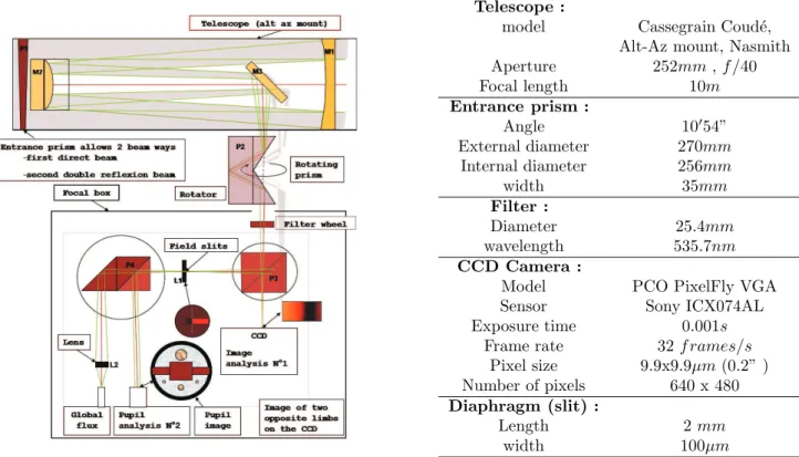
The Angle-of-Arrival fluctuations, which are fluctuations of the normal to the perturbed wavefronts, can directly be observed in the image plane (this is the case of Shack-Hartmann’s sensors currently used in the adaptive optics systems). But, they can also be shown in the pupil plane, for example, when the astronomical sources observed (Sun or Moon) present an intensity distribution with a strong discontinuity.5 _{In this case, an analysis} of the perturbed wavefronts analog to a Foucault test can be performed. Figure 1 shows the principle of the monitor experimental device. It consists in 2 ways.

Telescope :

model Cassegrain Coud´e, Alt-Az mount, Nasmith Aperture 252mm , f /40 Focal length 10m Entrance prism : Angle 10′ 54” External diameter 270mm Internal diameter 256mm width 35mm Filter : Diameter 25.4mm wavelength 535.7nm CCD Camera :

Model PCO PixelFly VGA Sensor Sony ICX074AL Exposure time 0.001s

Frame rate 32 f rames/s Pixel size 9.9x9.9µm (0.2” ) Number of pixels 640 x 480 Diaphragm (slit) :

Length 2 mm width 100µm

Figure 1. MISOLFA, Optical scheme and instrumental characteristics.

The first one, named in the following image plane observation way, allows recording directly the AA-fluctuations using a CCD camera placed on the solar limb image (No_{1). Observations taken from this way} are similar to those made by the Monitor of Outer Scale Profile (MOSP).6 _{A beam splitter allows to create a} second way, named in the following pupil plane observation way, in which the telescope pupil (P1) is observed by means of a lens through a narrow slit placed on the solar limb image (No_{2). The diaphragm size is 2 arc-seconds} wide and 40 arcseconds length. The pupil image intensity present fluctuations which are proportional to the AA-fluctuations (see section 4). Several photodiodes allow recording the intensity fluctuations with optical fibers positioned on the image behind diaphragms of different sizes. Signals given by the different photodiodes are si-multaneously recorded and a spatiotemporal analysis performed. The components and instrumental parameters of MISOLFA are summarized in the table of Figure 1.

2.2 Measurement principle - Theoretical models and turbulence parameter estimation

2.2.1 The image plane observation way

The theoretical basic equations were presented in more details in our past papers by Irbah et al.7, 8 _{and Corbard} et al.9 _{It’s obtained in the same way than those used to interpret the nighttime observation data given by the} Generalized Seeing Monitor.10, 11 _{Let’s recall the basic equation of the transverse spatial structure function of} the AA-fluctuations observed in a telescope of diameter D, where the atmospheric turbulence is described by the Von K`arm`an model:12

D_{α(θ) = 0.1432λ}2_r− 5 3 0 Z +∞ 0 df f3_(f2₊ 1 L₀2) −11 6[1 − J 0(2πf θh) − J2(2πf θh)][ 2J1(πDf ) πDf ] 2 ₍₁₎

f is an angular frequency, λ the wavelength, Jn are Bessel functions of the first kind, h is the altitude of an equivalent impulse layer giving the same optical effects at ground level than the whole turbulent terrestrial atmosphere (one layer model).

From MISOLFA observations, we can build an experimental structure function (see section 4.1.1). A subsequent non linear fit with Equation 1 leads to estimated values for the Fried parameter r0, the spatial coherence outer scale L0and the isoplanatic angle θ0.13

In the case of the multilayer model, Equation 1 becomes:

D_{α(θ) = 2.4sec(z)} Z +∞ 0 dhC2 n(h) Z +∞ 0 df f3_(f2₊ 1 L0(h)2 )−11 6[1 − J 0(2πf θh) − J2(2πf θh)][ 2J1(πDf ) πDf ] 2 ₍₂₎ where C2

n(h) is the structure constant for the air refractive index fluctuations, L0(h) is the turbulent outer scale vertical profile and z is the zenithal distance.

As a first approach we can consider the case in which L0(h) = ∞ for which the optical turbulence profile C2

n(h) can be estimated by application of the inversion technique described in Bouzid et al.14 2.2.2 The pupil-plane observation way

The main purpose of observing intensity fluctuations at high cadence (1 KHz) in the pupil plane is to estimate the turbulence characteristic time. However, it is also possible to reach again the spatial parameters (r0and L0). Previous works have effectively shown the good linear relationship between intensity fluctuation of flying shadows observed in the pupil plane and AA-fluctuations from both theoretical background and observations.8, 15–17

The use of a diaphragm of finite size in the focal plane introduces additional effects which limit AA-fluctuation analysis from intensity measurements of the pupil-plane images. Two effects were highlighted and have been studied by Borgnino and Martin.15, 16 _{They are related to the diffraction and angular filtering by the diaphragm.} Thus, the presence of a diaphragm with an angular width wx in the focal plane is equivalent to a high spatial frequency filter with a cut-off frequency fd given by :

fd≈ wx

λ (3)

However, geometrical considerations allow to say that details in a turbulent layer situated at an altitude h have spatial dimensions on the pupil plane of about hwx. We can then define a spatial cut-off frequency fa for the anisoplanatism angular filter as :

fa≈ 1 hwx

(4)

Borgnino and Martin15, 16 _{have shown that the best compromise is to put f}

a = fd. This allows us to chose various diaphragm dimensions in order to reach different altitudes. For a slit having an angular width equal to 2 arcseconds (see table on Figure 1) and for observations in the visible ( 535 nm), the filtering by diffraction is dominating until a height h=5 km. This filtering of the elements lower than 5cm in size is the same whatever is

the height from 0 to 5 km. For higher altitudes, it is the angular filtering which becomes dominant. For example, for h=6 km, the slit, because of the angular filtering, filters all the elements of size lower than 6cm. For h=7 km, all the elements of size lower than 7cm will be filtered. In a synthetic way, we find the effect of the 2 filterings in Figure 7 of Borgnino J. and Martin F. (1977).15

The spatial coherence parameters r0 and L0 may be obtained with the pupil-plane observation way together with AA fluctuation characteristic times. The structure function of AA fluctuations recorded by mean of a pair of photodiodes positioned in the pupil image may be expressed as:18

dα(s) = 0.364[1 − k( s Dp )−13]λ2r 0 −5 3D p −1 3 (5)

where k is a constant respectively equal to 0.541 or 0.810 according that we consider AA projected on the baseline formed by the photodiodes separated by the distance s or onto a perpendicular direction. Dpis the area integration size of the photodiodes. Equation 5 will be used to calculate r0.

The spatial coherence outer scale L0 may be deduced from the equation of the angular covariance for θ equal to 0. The integration gives in this case and considering that L0 is great in regard to Dp:19

C_{α(0, Dp) = 0.017λ}2_r0−53[D− 1 3 p −1.525L0 −1 3] (6)

The L0parameter will be obtained from Equation 6 applied to 2 photodiodes of different area integration sizes D_p1and D_p2. It will be obtained from the ratio rL0:

rL0 = C_{α(0, D} p1) − Cα(0, D_p2) C_{α(0, D} p1) = Dp1 −1 3 −D p2 −1 3 D_p1−1 3 −1.525L 0 −1 3 (7)

3. NUMERICAL SIMULATIONS

In order to check turbulence parameters extraction method from MISOLFA data processing, we performed numerical simulations. From shoosen parameters of Von K`arm`an model, we simulated a phase screen, generate a MISOLFA image through it, extract turbulence parameters and compare them to injected parameters.

The turbulent phase screen is obtained using Nakajima method.20 _{Optical perturbations from this method} are the inverse Fourier Transform of a random complex quantity which statistical variance is taken equal to the theoretical one for to the considered model (Von K`arm`an). This method gives phase and amplitude fluctuations. A Fourier Transform is then applied to the resulting screen amplitude limited to the telescope pupil area in order to obtain the angular distribution of the complex amplitude K−_α→

0( −

→_{α ) in the focal plane.}

3.1 Image plane observation way

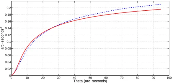
For simulating this way, we generate a solar image according to Hestroffer-Magnan21 _{and Mein (private} com-munication) center to limb darkening models, we add a poisson noise to it. A convolution product is then performed between this image and the complex amplitude cited above using a suitable sampling. The whole process is repeated for every incident angle of the angular domain allowed by the entrance pupil. A serie of 1000 images are simulated by randomly generating phase screens with the same input parameters (r0, L0 and h). The resulting images are processed following the same steps : edge detection, covariance and structure functions computing, non linear curve fitting according to Von K`arm`an model and using Levenberg-Marquardt method. We performed this simulation with high, medium and low turbulence corresponding to r0= 2cm, 5cm and 10cm. Figure 2 shows a result obtained with input parameters r0 = 10cm, L0= 60m and h = 8km. We can see that both theoritical and extracted structure functions have the same behaviour, so extracted parameters are in this case close to the input ones but more work is needed in order to assess the robustness of the method and check for possible bias in estimated parameters.

3.2 Pupil plane observation way

In this case, as described by Berdja et al.,17 _{the diaphragm effect is simulated by keeping a randomly part of} the complex amplitude K−_α→

0( −

→_{α ). As for the image plane, the process is repeated for every incident angle, the} resulting image presents flying shadows. An example of flying shadows is shown in Figure 3 and simulations were carried out by Berdja et al.17

0 10 20 30 40 50 60 70 80 90 100 0 0.02 0.04 0.06 0.08 0.1 0.12 0.14 0.16 0.18 0.2 Theta (arc−seconds) arc−seconds 2

Figure 2. Simulated (dashed line) and theoretical (solid line) AA-structure functions observed in image plane. The perturbed wave-front was simulated in the near-field approximation case considering r0= 10cm, L0= 60m, h = 8000m.

Figure 3. Simulated AA-fluctuations computed directly from the perturbed wave-front phase and observed as intensity fluctuations in pupil-plane image. (a) and (b) are respectively x and y AA components at the entrance pupil while (c) is the y component observed in the pupil-plane image as intensity fluctuations. The perturbed wave-front was simulated in the near-field approximation case considering r0= 4cm, L0 = 10m, h = 1000m. The diaphragm width was taken equal

to few arc-seconds.

3.3 Effect of Fried parameter on Solar diameter measurements using SODISM II

We performed numerical simulations to show the effect of Fried parameter on solar diameter measurement directly carried out on a full solar image such as recorded by SODISM II. Exposure time of SODISM II images at 535 nm is 1.3 s. Knowing that typical turbulence characteristic time (τ0) is lower than 100 ms, SODISM II images can be considered as long-exposure images. The effect of Fried parameter on SODISM II measurements can be simulated in two ways. The first one consists in a convolution of the simulated image by a point spread function (psf) obtained with an equivalent diameter equal to r0. The diameter is then measured from the resulting image and compared with the original one. The result of this operation is the well known limb spread wich correspond to a lowering of the inflection point position and thus a shorter diameter as r0 decreases. A bias can thus be estimated as a function of r0.

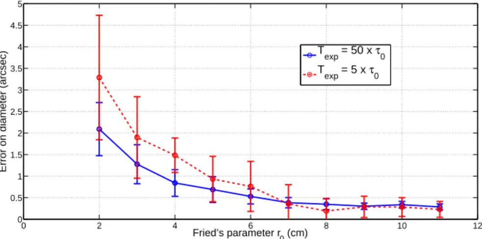
The second option is similar to the procedure used to simulate MISOLFA images. We convolve a theoretical SODISM II image with a generated phase screen corresponding to the state of the atmosphere in a time equal or less than τ0. By averaging several of the simulated images, we simulate different exposure times. The diameters are obtained by the zero crossing of the second derivative of the obtained limb. The systematic errors in diameter measurement are then obtained by substracting the original diameter. From these Monte-Carlo simulations, we

0 2 4 6 8 10 12 0 0.5 1 1.5 2 2.5 3 3.5 4 4.5 5 Fried’s parameter r 0 (cm)

Error on diameter (arcsec)

T

exp = 50 x τ0 T

exp = 5 x τ0

Figure 4. Simulation of the error due to Fried parameter r0on solar diameter measurement with SODISM II, Von K`arm`an

model was assumed to simulate the phase screens with an infinite value of the outer scale. Exposure time is simulated by varying the number of images taken to compute the diameter.

obtain not only the bias introduced by r0on the diameter measurements, but also an estimate of the statistical error on this bias as a function of r0. In addition, this method allows us to simulate different ratios betweeen exposure time and τ0.

Figure 4 clearly shows that the systematic error decreases as r0 increases. The full line represents long exposure times (50 x τ0) which most likely corresponds to SODISM II images while the dashed line corresponds to a shorter exposure time (5 x τ0). As expected, the statistical error bars obtained from Monte-Carlo simulations are bigger for short exposure times when the corresponding PSF still show speckle structures rather than the smooth function corresponding to long exposure images. This illustrates the importance of measuring also τ0. We can also see that when r0 increases and approaches the telescope diameter, the observations are diffraction limited.

4. RESULTS ON FRIED PARAMETER ESTIMATE AND DISCUSSIONS

Some preliminary results were presented by Irbah et al.,7, 8 _{Corbard et al.}9 _{and Ikhlef et al.}22

4.1 Data processing steps

4.1.1 Image-plane measurements

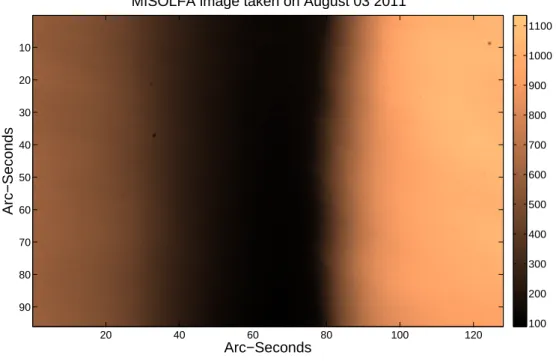
Data consist in image series of about 2400 samples recorded at a rate of 32 per second. According to Martin et al.1987, exposure time of the detector is a crucial parameter for seeing studies. It should be shorter than 0.01 s to freeze the atmospheric image motion.23 _{Thus, the exposure time of the video ccd camera is adjusted to a constant} value of 0.001 s. Figure 5 shows an image of the Sun recorded on August 03, 2011 with this observation way. Its size is approximately 96 by 128 arc-seconds. Each CCD pixel line in the direct and reflected limb images are such as they are located on a direction parallel to the local horizon. For each limb, the following step are performed: noise estimation using Standard Deviation Histogram Algorithm (SDHA, see Gao et al.24_{), image cleaning by} wavelet denoising process, edge detection, correction from medium edge, cross-corelation computation. AA-fluctuations are extracted from temporal series of solar images allowing to compute the experimental covariance function Cα_⊥Exp(θ) and the structure function dα_⊥Exp(θ) which equation is given by:6

dα_⊥Exp(θ) = 1 N N X i=1 1 θm−θ θXm−θ k=1 [α⊥(k) − α⊥(k + θ)]2 (8)

Arc−Seconds

Arc−Seconds

MISOLFA image taken on August 03 2011

20 40 60 80 100 120 10 20 30 40 50 60 70 80 90 100 200 300 400 500 600 700 800 900 1000 1100

Figure 5. A solar image obtained with the image-plane observation way of MISOLFA. On the left the reflected limb and the direct limb is on the right.

where θ is the angular separation in pixels, θmis the maximal extent accessible in the image (i.e. 480 pixels in our case), N is the number of processed images (about 2400) and α⊥(k) is the AA-fluctuations retrieved at the position k.

The Fried parameter r0, the spatial coherence outer scale L0 and the altitude of the equivalent impulse layer h are then estimated fitting dα⊥Exp(θ) with the theoretical model given by Equation 1.

However, in the case of great values of the outer scale L0, one can considerer the Kolmogorov model for r0 estimation:2, 3 r0= 8.25 105λ 6 5D− 1 5σ α −6 5 (9)

where the standard deviation σαof the limb position is expressed in arc-seconds.

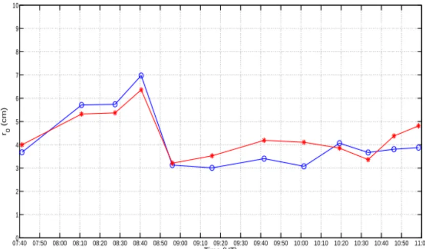
In practice we use the standard deviation of the summit of parabola fitting the limb edges. Figure 6 presents r0 measurement during one day (July 28th 2011).

In order to obtain a stable estimate of r0, a full serie of 2400 images spanning 1.5 mn was used for each r0 estimate. In order to achieve this we had to remove all long term trends or discontinuities due to intrumental effects, wind, etc... rather than turbulence.

Previous work have shown that using MISOLFA images spanning only 2 s (i.e roughly SODISM II exposure time) and without removing instrumental trends, one obtain strong and probably unrealistic fluctuations in r0 estimate.

4.1.2 Pupil-plane measurements

Light fluctuations in the pupil plane are converted to electrical signals by photodiodes. A low noise electronic amplification device and a data acquisition system are used to acquire these signal at a rate of 1 KHz. Temporal covariance functions are then obtained by cross-correlation of these signals. Some preliminary results from this observation way were presented and discussed by Irbah et al.8

07:40 07:50 08:00 08:10 08:20 08:30 08:40 08:50 09:00 09:10 09:20 09:30 09:40 09:50 10:00 10:10 10:20 10:30 10:40 10:50 11:000 1 2 3 4 5 6 7 8 9 10 Time (UT) r0 (cm)

Figure 6. Fried parameter estimation measured on July 28 2011 from direct (circles) and reflected (stars) limbs.

4.2 Statistics of Fried parameter measurements since June 2010

Fried parameters obtained with MISOLFA between June 23 2010 and May 16 2012 are shown in the left side of Figure 7, observations were done one or two days a week, according to meteorogical conditions, we have 10-30 observation files a day (multifits files of 2400 images).

Apr100 Jul10 Oct10 Jan11 Apr11 Jul11 Oct11 Jan12 Apr12 Jul12

2 4 6 8 10 12 r0 (cm) 1 2 3 4 5 6 7 8 9 10 11 12 0 0.5 1 1.5 2 2.5 3 3.5 4 4.5 r0 (cm) months

Figure 7. Fried parameter measurement performed between 06/23/2010 and 05/16/2012, on the left estimation of r0from

reflected (stars) and direct (circles) limbs, on the right r0 monthly median values for this period.

Because of the degradation of the coating on the prismatic entrance window, we don’t have data from reflected limb during the whole period. We are now studying this problem and looking for a best quality and long term efficiency of the coating.

Cumulative frequency distribution of Fried parameters is demonstrated in figure 8. We can see that 15% of measured Fried parameters are larger than 5 cm. The median value over the whole period (June 2010 to May 2012) is 3.5 cm and 3.42 cm for the reflected and direct limb measurents respectively. These values are significantly less than those measured by night-time at Calern Observatory10_{with DIMM and GSM instruments.}

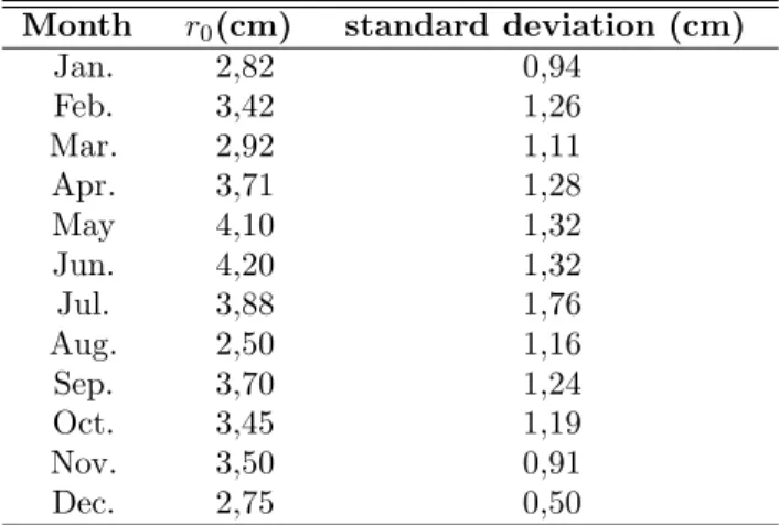
On the right side of Figure 7 and on Table 1, we present monthly Fried parameter median values over the two years and its standard deviation, we can see that the best measurements were obtained on June for which median value is larger than the mean over the whole period (June 2010 to May 2012). For this particular month, we see that more than 50% of measured r0 are larger than 4 cm and less than 10% larger than 8 cm. The mean

Month r0(cm) standard deviation (cm) Jan. 2,82 0,94 Feb. 3,42 1,26 Mar. 2,92 1,11 Apr. 3,71 1,28 May 4,10 1,32 Jun. 4,20 1,32 Jul. 3,88 1,76 Aug. 2,50 1,16 Sep. 3,70 1,24 Oct. 3,45 1,19 Nov. 3,50 0,91 Dec. 2,75 0,50

Table 1. Monthly median Fried parameter r0 and its standard deviation between 06/23/2010 and 05/16/2012.

0 1 2 3 4 5 6 7 8 9 10 0 10 20 30 40 50 60

Fried’s parameter estimation histogram from direct limb

r₀ (cm) counts 1 2 3 4 5 6 7 8 9 10 11 0 5 10 15 20 25 30 35

Fried’s parameter estimation histogram from reflected limb

r

0 (cm)

counts

Figure 8. Fried parameter histograms of measurements performed between 06/23/2010 and 05/16/2012.

observed zenithal distance changes over time and thus also influence our monthly values. We can also say that best seeing quality is observed in the morning but most stable seeing conditions often occur in the afternoon.

5. CONCLUSION

In order to understand atmospheric turbulence effects on solar astrometric observations and specially solar diameter, MISOLFA was developed. It estimates the spatio-temporal parameters and observes simultanuousely with the replica of the space instrument SODISM onboard of PICARD satellite. We presented here Fried parameter statistics of measurements performed with image plane observation way of MISOLFA since June 2010. We have also shown through simulations how this parameter can be used in analyzing SODISM II images by providing an estimate of the bias and statistical error induced by turbulence on diameter measurements. Indeed, we need more parameters estimation to better understand atmospheric effects, the spatial coherence outer scale L0 , isoplanatic angle θ0 and the vertical optical turbulence profile Cn2(h) will be estimated from inversion of structure function obtained with these data. The use of pupil plane observation will allow us to measure both spatial and temporal parameters.

ACKNOWLEDGMENTS

The data were provided by the PICARD instrument team. PICARD is a mission supported by the Centre national d’Etudes Spatiales (CNES), the CNRS/INSU, the Belgian Space Policy (BELSPO), the Swiss Space Office (SSO) and the European Space Agency (ESA).

REFERENCES

[1] Morand F., Delmas C, Corbard T., Chauvineau B., Irbah A., Fodil M. and Laclare F., “Mesures du rayon solaire avec l’instrument DORAYSOL (1999-2006) sur le site de Calern (Observatoire de la Cˆote d’Azur)”, C. R. Acad. Sci. Paris, 660-673, 2010.

[2] Irbah A., Laclare F., Borgnino J. and Merlin G.,“Solar diameter measurements with Calern Observatory astrolabe and atmospheric turbulence effects”,Solar Phys., 149, 213, 1994.

[3] Borgnino J., Ricort G., Ceppatelli G. and Righini A., “Lower atmosphere and solar seeing - an experiment of simultanuous measurements of nearby turbulence by thermal radiosondes, by angle of arrival statistics and image motion observation”, Astron. Astrophys. 107, 333, 1982.

[4] Lakhal L., Irbah A., Bouzaria M., Borgnino J., Laclare F., Delmas C., “Error due to atmospheric turbulence effects on solar diameter measurements performed with an astrolabe”,Astron. Astrophys. Suppl. Ser., 138, 155, 1999.

[5] Irbah A., Borgnino J., Laclare F., and Merlin G., “Isoplanatism and high spatial resolution solar imaging”, Astron. Astrophys., 276, pp. 663–672, 1993.

[6] Maire J., Ziad A., Borgnino J., Martin F., “Measurements of profiles of the wavefront outer scale using observations of the limb of the Moon”, Mon. Not. R. Astron. Soc., 377, pp. 1236–1244, 2007.

[7] Irbah, A., Corbard, T., Assus, P., Borgnino, J., Dufour, C., Ikhlef, R., Martin, F., Meftah, M., Morand, F., Renaud, C. & Simon, E., “The solar seeing monitor MISOLFA: presentation and first results”, SPIE Conference Series, p. 211, 2010.

[8] Irbah A., Meftah M., Corbard T., Ikhlef R., Morand F., Assus P., Fodil M., Lin M., Ducourt E., Lesueur P., Poiet G., Renaud C. & Rouze M., “Ground-based solar astrometric measurements during the PICARD mission”, SPIE Conference Series, 2011.

[9] Corbard, T., Irbah, A., Assus, P., Dufour, C., Fodil, M., Morand, F., Renaud, C. and Simon, E., “MISOLFA solar monitor for the ground PICARD program”, Astron. Nachr., 2011.

[10] Martin F., Tokovinin A., Agabi A., Borgnino J. and Ziad A., “G.S.M.: a grating scale monitor for atmo-spheric turbulence measurements. I. The instrument and first results of angle of arrival measurements”,Astron. Astrophys. Suppl. Ser., 108, pp. 173–180, 1994.

[11] Ziad A., Conan R., Tokovinin A., Martin F., and Borgnino J., “From the Grating Scale Monitor to the Generalized Seeing Monitor,” Applied Optics 39, p. 30, 2000.

[12] Avila R., Ziad A., Borgnino J., Martin F., Agabi A. and Tokovinin A., “Theoretical spatio-temporal analysis of angle of arrival induced by atmospheric turbulence as observed with the Grating Scale Monitor Experi-ment,” J. Opt. Soc. Amer. A 14, p. 11, 1997.

[13] Seghouani N., Irbah A. and Borgnino J., “Estimation of the spatial coherence outer scale for daytime observations”, Marrakech Site 2000, Astronomical Site Evaluation in the Visible and Radio Range, Marrakech - Morocco, November 13-17, 2000.

[14] Bouzid A., Irbah A., Borgnino J. and Lantri H., “Atmospheric turbulence profiles Cn2(h) deduced from solar limb observations”, Marrakech Site 2000, Astronomical Site Evaluation in the Visible and Radio Range, Marrakech - Morocco, November 13-17, 2000.

[15] Borgnino J., and Martin F., “Analyse statistique des d´eformations al´eatoires d’une surface d’onde dues `a la turbulence atmosph´erique au voisinage du sol, I.- Expos´e de la m´ethode, Premiers r´esultats,” J. Optics (Paris) 8, pp. 319–326, 1977.

[16] Borgnino J., and Martin F., “Analyse statistique des d´eformations al´eatoires d’une surface d’onde dues `a la turbulence atmosph´erique au voisinage du sol, II.- Estimation des fonctions de corr´elation par traitement num´erique,” J. Optics (Paris) 9, pp. 15–24, 1977.

[17] Berdja A., Irbah A., Borgnino J., and Martin F., “Simulmation of pupil-plane observation of angle-of-arrival fluctuations in daytime turbulence, in Optics in Atmospheric”, Propagation and Adaptive Systems VI, edited by John D. Gonglewski and Karin Stein, Proceedings of SPIE Vol. 5237 (SPIE, Bellingham, WA, 2004), p. 238-248, 2004

[18] Sarazin M. and Roddier F., “The ESO differential image motion monitor”, Astron. and Astrophys., 227, p. 294-300, 1990

[19] Ziad A., Borgnino J., Martin F. and Agabi A., “Experimental estimation of the spatial coherence outer scale from a wavefront statistical analysis”, Astron. and Astrophys. 282, p. 1021-1033, 1994

[20] Nakajima T., ”Signal-to-noise ratio of the bispectral analysis of speckle interferometry”, J. Opt. Soc. Am. A.5: 963-985, 1988

[21] Hestroffer D., Magnan C., ”Wavelength dependency of the solar limb darkening”, Astron. Astrophys., Vol. 333, pp. 338-342, 1998

[22] Ikhlef R., Corbard T., Irbah A., Meftah M., Morand F., Fodil M., Assus P., Renaud C., Chauvineau B. and The whole Picard-Sol team, ”MISOLFA: A seeing monitor for daytime turbulence parameters measurements” 4th French-Chinese Meeting on Solar Physics, EAS Publication Series Vol. 55, 2012

[23] Martin, H. M. 1987, “Image motion as a measure of seeing quality”, PASP, Vol. 99, pp. 1360-1370, 1987. [24] Gao B. C., “Operational method for estimating signal to noise ratios from data acquired with imaging