HAL Id: hal-00299373
https://hal.archives-ouvertes.fr/hal-00299373
Submitted on 6 Oct 2006
HAL is a multi-disciplinary open access
archive for the deposit and dissemination of
sci-entific research documents, whether they are
pub-lished or not. The documents may come from
teaching and research institutions in France or
abroad, or from public or private research centers.
L’archive ouverte pluridisciplinaire HAL, est
destinée au dépôt et à la diffusion de documents
scientifiques de niveau recherche, publiés ou non,
émanant des établissements d’enseignement et de
recherche français ou étrangers, des laboratoires
publics ou privés.
S. de Zolt, P. Lionello, A. Nuhu, A. Tomasin
To cite this version:
S. de Zolt, P. Lionello, A. Nuhu, A. Tomasin. The disastrous storm of 4 November 1966 on Italy.
Natural Hazards and Earth System Science, Copernicus Publications on behalf of the European
Geo-sciences Union, 2006, 6 (5), pp.861-879. �hal-00299373�
www.nat-hazards-earth-syst-sci.net/6/861/2006/ © Author(s) 2006. This work is licensed under a Creative Commons License.
and Earth
System Sciences
The disastrous storm of 4 November 1966 on Italy
S. De Zolt1, P. Lionello2, A. Nuhu3, and A. Tomasin4
1Department of Physics, University of Padua, via Marzolo 8, 35131 Padua, Italy
2Department of Materials Science, University of Lecce, via Arnesano, 70300 Lecce, Italy 3Department of Physics, University of Padua, via Marzolo 8, 35131 Padua, Italy
4Department of Applied Mathematics, University “Ca’ Foscari” and ISMAR-CNR, San Polo 1364, 30125 Venice, Italy
Received: 5 April 2006 – Revised: 14 September 2006 – Accepted: 21 September 2006 – Published: 6 October 2006
Abstract. This is the first modeling reconstruction of the
whole aspects (both meteorological and oceanographic) of the storm which hit Italy on 4 November 1966, produc-ing 118 victims and widespread damages in Tuscany, at the northern Adriatic coast and in the north-eastern Italian Alps. The storm was produced by a cyclone which formed in the western Mediterranean and moved eastward towards Italy, reaching the Thyrrenian Sea, and then northward. The most peculiar characteristic of the storm has been the strong zonal pressure gradient and the consequent intensity and long fetch of the south-easterly sirocco wind, which advected a large amount of warm moist air, and determined exceptional orographic precipitation over Tuscany and the north-eastern Alps. The funneling of the wind between the mountain chains surrounding the Adriatic basin further increased the wind speed and determined the highest ever recorded storm surge along the Venetian coast.
This study shows that present models would be able to pro-duce a reasonably accurate simulation of the meteorological event (surface pressure, wind and precipitation fields, and storm surge level). The exceptional intensity of the event is not suggested by single parameters such as the sea level pressure minimum, the wind speed or the total accumulated precipitation. In fact, the precipitation was extreme only in some locations and the pressure minimum was not partic-ularly deep. Moreover, the prediction of the damages pro-duced by the river run-off and landslides would have required other informations concerning soil condition, snow coverage, and storage of water reservoirs before the event. This indi-cates that an integrated approach is required for assessing the probability of such damages both on a weather forecast and on a climate change perspective.
Correspondence to: S. De Zolt ([email protected])
1 Introduction
During the first days of November 1966 an extreme mete-orological event caused huge damages in several areas of northern and central Italy. The situation was extraordinary for its intensity, duration, and the extent of the overall areas that were heavily affected. Two different kinds of phenom-ena, associated with the same meteorological situation, con-tributed to the exceptionality of the event: the intense and prolonged precipitation, which caused hydrological and ge-ological damages in both central and north-eastern Italy; the large wind speed and the consequent combination of high waves and storm surge level, which hit the northern coast of the Adriatic Sea. This study aims to provide a complete re-construction of this storm, including both meteorological and oceanographic aspects.
The extreme event was caused by the development and intensification of a baroclinic wave over Europe and the Mediterranean, associated with a strong meridional temper-ature gradient: this situation created favorable conditions for cyclogenesis and determined a strong meridional transport of heat and specific humidity. The cyclone formation is evi-dent from the presence of a minimum in the SLP (Sea Level Pressure) maps on 3 November over the western Mediter-ranean basin, which successively moved eastward towards Italy, where it produced the large precipitation over Tus-cany. Then it followed a more northern path so that southerly winds blew along the Adriatic towards the eastern sector of the Alps, causing intense precipitation in the north-eastern regions, mainly on the southern side of the Alps, and high waves and storm surge in the northern Adriatic Sea. More-over, the presence of an anticyclone north of the Black Sea determined a very strong zonal pressure gradient, and fa-vored intense southerly winds, which, in the Adriatic sea, were further reinforced by the channeling due to the moun-tain ridges surrounding the basin. The exceptional storm surge level reached in the northern part of the Adriatic was
Venice Ravena Genoa Falconara Florence Grosseto Civitavecchia Bari Streams overflow
landslides Highest recorded Trento flood precipitation (751 mm) Tagliamento: countriside flooded 14 victims Maximum ever recorded surge Po delta: distruction of coastal defences Arno overflow: Florence flood, 38 victims Ombrone overflow: flood of Maremma Trento Adige Overflow: 22 victims
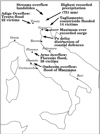
Fig. 1. Map of the damages produced by the 4 November 1966
storm. The locations of the the towns mentioned in the paper are also reported.
caused by the intensity and persistence of this wind. After 5 November phenomena ceased over Italy, as the cyclone moved further north-eastward and was reabsorbed by a large system passing above central Europe.
Observations of meteorological and marine variables, like sea level pressure, wind, precipitation, sea level, obtained from station measurements, radiosoundings and radar data, can be used to understand the dynamics of the event. Nev-ertheless, they are not sufficient to describe entirely the sit-uation. Further data have to be provided by global model re-analysis, such as ERA-40 and NCEP, and regional model simulations. Global re-analysis data are available with a rel-atively low resolution, approximately 130 km in the dataset with higher resolution (ERA-40). In order to better describe the physical processes and the dynamics of the event it is use-ful to analyse higher resolution data which can be provided by a numeric integration with a regional model. In this study model simulations at about 30 and 10 km resolution are used. Such models are a tool for understanding the event. How-ever, an important point is to test their capability of repro-ducing its extreme intensity, that is the intense precipitation and wind, and the consequent floods, storm surge and high
waves. Furthermore, such limited area models allow to test different modalities of describing physical processes in order to understand their role. Finally, the importance of the im-posed initial and boundary conditions can be analysed. As a result this paper aims at evaluating whether such event could be well simulated with the regional models that are presently available and what would be the main sources of uncertainty. A last point is the identification of the features responsible for the exceptionality of the event.
Section 2 contains a description of the casualties and dam-ages that were produced by the storm. In Sect. 3 the regional models (both meteorological, storm surge and wave models) used to perform the experiments are presented, and the char-acteristics of the simulations and of the data used for valida-tion are described. Sect. 4 contains a synoptic and mesoscale description of the extreme event. The analysis of the results and the comparison with available observations is contained in Sect. 5. It considers a set of atmospheric variables: precip-itation, SLP (Sea Level Pressure), U10 (wind at 10 m level) and GPH500 (GeoPotential Height of the 500 hPa pressure surface). Besides them, sea elevation and SWH (Significant Wave Height) fields are analysed. In Sect. 6 the role of the various modeling features for the simulation of the event is discussed, and the exceptionality of the phenomena is anal-ysed from a statistical point of view. Finally, the conclusions are presented.
2 Damages
The damages caused by the event were serious all over north-ern and central Italy, where it caused 118 victims (APAT, 2004). However, the impact of the storm was disastrous on four main areas (Fig. 1): central Italy (Tuscany), the east-ern sector of the Alps, the north-easteast-ern Italian Plane (Pia-nura Veneto-Friulana), the northern Adriatic coast (including Venice and its lagoon). In the first three regions the damages were caused by the very heavy precipitation, in the fourth one by the high waves and storm surge.
2.1 Central Italy
The region where the consequences of the storm were most severe is Tuscany, where the return times associated to the recorded precipitation are higher than 50 years at several locations (see Sect. 6). Precipitation maxima were located in the Arno’s and Ombrone’s catchment basins. The maxi-mum value of 437.2 mm for the precipitation accumulated in two days was observed in the Arno’s basin (Bendini, 1969). The persistent precipitation of the previous months, that was more than 150% higher than average (Gazzolo, 1969), played an important role in determining the floods, because the stor-age capacity of the rivers and of the soil was very low already before the storm took place. The rivers discharge reached ex-ceptional levels for all the Arno’s tributaries, with dramatic
consequences in all its basin, where villages and the coun-tryside were flooded. About 70 km upstream of Florence along the Arno, the estimated river’s discharge was higher than 2250 m3s−1, corresponding to more than 250% of the maximum estimated value in the preceding 30 years (Ben-dini, 1969). In Florence the Arno broke its banks and the water invaded the town and reached 4.93 m above the ref-erence level, 33 cm higher than the previous record which took place in 1333. In some places of the town, the wa-ter overpassed the 6 m height. Damages were huge. Local newspapers report that 38 people died. The gas, electric-ity and water supply were completely cut off. The indus-trial areas of the region around Florence were flooded and all the equipment was severely damaged. In addition to the economical losses, Florence suffered for the ruin of highly valuable artistic goods: 14 000 movable works of art were destroyed, more than 3 million books and manuscripts were damaged and many valuable artistic buildings of the town were spoiled.
Damages were huge also in Maremma, where the Om-brone river flooded an area more than 300 km2 wide, in-cluding Grosseto and the countryside around. The road and railway networks and the hydrographic system were partially destroyed, but the most considerable losses were suffered by the agricultural and zootechnical goods.
2.2 Eastern Alps
The highest precipitation amount, during the 4 November 1966 storm, fell over the eastern Alpine and pre-Alpine ar-eas. Many stations recorded more than 400 mm of precipita-tion accumulated in two days, with 751.4 mm as the highest value reached (Dorigo, 1969). Also in this region, the situ-ation was particularly critical because of the prolonged and large precipitation of the previous months, which brought the storage capacity of deep and surface soil next to saturation. Snow had fallen abundantly on the Alps and, due to the sud-den temperature rise caused by the southerly wind flow dur-ing the event, it partially melted, further increasdur-ing the load of water on streams and soil. Ruin was wide spread in many valleys, where streams overflew and swiped away houses and bridges, and numerous landslides isolated the villages for several days. Huge economical damages were caused by the destruction of thousands of houses, cars and industrial equip-ments, loss of goods, cattle and crops. The consequences included overflood of the drainage system, lack of potable water and destruction of electric supply system.
In Trento, the Adige’s discharge reached 2320 m3s−1, and the river broke its banks in several points (Dorigo, 1969). The town and 5000 ha in the countryside and valleys around it were flooded. The victims were 22 in the district and dam-ages were estimated 68 billions lire (about 680 millions of present-day Euro1). In Trento the 6.30 m level above the
ref-1This and following evaluations accounted for the about 20-fold
erence was reached, surpassing the previous record of 6.11 m established by the flood of 1882. Fortunately, the Adige flood was limited to the northern part of the basin, because downstream of Trento its water was deviated into the Garda lake through the Adige-Garda gallery, where 67 millions cu-bic meters of water were discharged, corresponding to a rise of 18 cm of the lake level.
2.3 Venetian-Friuli Plane
Big damages were caused by almost all the rivers cross-ing the plane, whose discharge in most cases overtook the maxima of the previous observation period, producing widespread floods.
The largest damages were produced by the Tagliamento river, whose level had been growing more than 0.5 mh−1 reaching a maximum of 10.88 m above the mean level about 10 km north of its estuary (Dorigo, 1969). The river flooded 22 000 ha in the countryside around it across 4 main break-ing points in its bank. Because of the event 14 people were killed, 5000 left homeless. The damage has been estimated 77 billions Italian Lire (not including the cost of repairing the banks), corresponding to about 770 millions of present day Euros. The extreme intensity of the event can be evalu-ated considering that the peak transport was estimevalu-ated about 4000 m3s−1, while the mean value is about 90 m3s−1, and the 10-year return value is 2580 m3s−1.
2.4 North Adriatic coast
Coastal areas of the northern Adriatic were threatened by the strength of the sea waves, and in many places coastal de-fences were destroyed. In the area around the Po’s delta, about 10 000 ha of countryside were covered by 2 m of salty water, that made the land infertile for several years and killed cattle, with consequent huge economical damages.
The city and the lagoon of Venice with its monumental and environmental heritage were hit by the highest surge ever recorded. The sea level raised about 170 cm above the mean sea level and persisted for more than 15 h above the 100 cm level (Canestrelli et al., 2001), which at that time corresponded to the critical value above which more than two thirds of Venice were flooded (Frassetto, 1976). The Novem-ber 1966 surge level was clearly exceptional and the return time is likely larger than 250 years (Lionello, 2005). Elec-tric power supply and telephone connections were cut off in Venice and in the islands of the lagoon. High waves swept the coastal defences and made a breach about 4 km wide through which the lagoon was temporarily joined to the Adriatic Sea. Though it was necessary to evacuate with motorboats about 4000 people from two coastal villages, fortunately, there were only three victims caused by the storm surge.
Eco-inflation which took place from 1966 to the beginning of the 21st century and the conversion from Italian currency to Euro in 2002.
nomic loss were evaluated about 40 billions of Italian lire, which are equivalent to about 400 million present-day Euros.
3 Models and simulations
In order to study both the marine and the meteorological as-pects of the November 1966 event, several regional models have been used: BOLAM, POM, HYPSE, WAM, MIAO, in-tegrated by a simple wave-current interaction model, named NSM. The following subsections contain a brief description of them.
3.1 BOLAM
BOLAM (Bologna Limited Area Model, Buzzi et al., 1994) is a meteorological limited area model, which integrates the primitive equations of the dynamics and thermodynamics of the atmosphere using wind velocity, pressure, specific humidity and potential temperature as prognostic variables. The model makes use of the hydrostatic approximation. It has vertical sigma coordinates and a vertical discretization of Lorentz’s type. On the horizontal surfaces discretization is performed on an Arakawa C-grid and using rotated geo-graphical coordinates. Horizontal diffusion is modelled by applying a square laplacian operator. A ”sponge layer” lim-its wave reflection at the top of the atmosphere. Boundary conditions are imposed every 6 h on the border of the do-main, and relaxed towards the centre of the dodo-main, using the 8 outermost frames.
Large scale precipitation and condensation processes are explicitly described using five types of hydrometeors. Mix-ing is simulated by the model in order to establish a neutral profile when the column of air reaches a vertical statically un-stable potential temperature profile. When the vertical profile of the column of air is convectively unstable, convective pro-cesses can be parameterized, following Fritsch-Chappell’s scheme (Kain and Fritsch, 1993): condensation and precipi-tation are computed and a stable or neutral vertical profile is produced. This is meant to prevent the development of con-vection on unrealistic spatial scales, which might occur when the model resolution is coarse. This parameterization can be switched-off and these processes can be explicitly described. Momentum, humidity and heat surface fluxes in the sur-face layer are parameterized following the Monin-Obukhov similarity theory. The model also includes a parameteriza-tion of radiative processes and interacparameteriza-tions with clouds. Soil physics is represented with a three-layer model which com-putes energy and water balance equations.
3.2 POM
POM (Princeton Ocean Model, Blumberg and Mellor, 1987) is a three-dimensional model describing the oceanic circu-lation. It uses horizontal curvilinear coordinates and an Arakawa C-grid. It has sigma vertical coordinates and a free
surface (Kantha and Clayson, 1995). Differentiation is im-plicit on the horizontal coordinate, exim-plicit on the vertical one. The integration technique is of “leap frog” type and needs an Asselin filter to prevent time splitting. The tech-nique named “mode splitting” allows to optimize comput-ing resources: fast movcomput-ing gravity waves and slower internal waves are integrated separately, with two different time steps. Faster waves are integrated in the external mode, with equa-tions describing the evolution of surface elevation and vol-ume transport. The vertical profile of temperature, salinity and velocity is computed in the internal mode with a lower frequency. The model contains a second order turbulence closure scheme for the computation of vertical mixing coef-ficients. It is particularly suitable to model mesoscale pro-cesses in coastal and estuary areas.
3.3 WAM
The WAM (the WAMDI group, 1988) wave model solves the energy transfer equation, which describes the variation of the wave spectrum in space and time due to the advec-tion of energy and local interacadvec-tions. The wave spectrum is locally modified by the input of energy from the wind, the redistribution of energy due to nonlinear interactions and en-ergy dissipation due to wave breaking and bottom friction in shallow water. The energy propagation and the integra-tion of the source funcintegra-tion are treated numerically using dif-ferent techniques. The advective term is integrated with a first order upwind scheme. The source function is integrated with an implicit scheme that allows an integration time step greater than the dynamic adjustment time of the highest fre-quencies in the model prognostic range. The wave spectrum is discretized using 12 directions and 25 frequencies extend-ing from 0.06114 to 0.41 Hz with a logarithmic increment
fn+1=1.1 fn. Beyond the prognostic region where the
en-ergy transfer equation is explicitly solved the spectrum is ex-tended by continuity with an f−5tail, which is necessary to compute the nonlinear interactions and the mean quantities occurring in the dissipation source function.
3.4 HYPSE
HYPSE (Hydrostatic Padua Sea Elevation model, Lionello et al., 2006) is a one layer shallow water model. Its prognostic equations are obtained by vertically integrating the equations of motion, with the hypothesis that variables have a constant value along the vertical coordinate. It uses curvilinear or-thogonal coordinates, an Arakawa-C differencing scheme, and uses a “leap frog” explicit scheme with an Asselin fil-ter. The model includes the astronomical tidal forcing, a quadratic bottom friction and Smagorinsky horizontal diffu-sivity. External forcing is represented by atmospheric pres-sure and wind stress, and, eventually, by prescribed time de-pendent conditions along the open boundary.
3.5 MIAO
The BOLAM, POM and WAM models described above can be coupled to each other in order to describe the feedback mechanisms from the ocean on the atmosphere at the air-sea interface. The MIAO model (Model of Interacting At-mosphere and Ocean, Lionello et al., 2003a) includes the three models as separated modules linked by a set of rou-tines coordinating the exchange of information and account-ing for the different grids and time steps of the models. BO-LAM computes atmospheric SLP, and the fluxes of momen-tum, heat, evaporation and precipitation at the air-sea inter-face, which are the upper boundary forcings for POM; it also computes the 10 m wind, that forces the wave model WAM. In turn, POM computes the SST (Sea Surface Temperature) and WAM the sea surface roughness used by BOLAM. This model framework automatically ensures a high frequency forcing, meaning that the exchange of information among modules takes place every 20 min, which consequently cor-responds to the time step of the forcing fields.
The model can also be used in the “one-way coupling modality”, where only the flux of information from the atmo-spheric model is active, while in the BOLAM model surface temperature above sea is prescribed and the surface rough-ness is computed with the Charnock formula.
3.6 NSM
The NSM (Near Shore Model, Lionello 1995) describes cur-rents and waves in the shallow water near the coast, account-ing for the strong effect of waves on the near-shore currents. The boundary conditions are provided by the results of the wave and the ocean circulation models that were described in the previous subsections. The model extends 11 km off-shore using a realistic bottom topography. The water depth is corrected accounting for tide and the meteorological set-up computed by the circulation model.
The model assumes a steady situation where the current in absence of the wave is small and the mean current gen-erated by the wave is depth independent. In the momentum equation the gradient of pressure associated with the slope of the sea surface balances the gradient of the wave radiation stress (Longuet-Higgins, M. S. and Stewart, R. W., 1962 and 1964) and the wind stress in the cross-shore direction, de-scribing the rise of sea level near the shore because of wave breaking (wave set-up) and a decrease of sea level further off-shore because of shoaling (wave set-down). The long-off-shore component of the momentum equation implies that the wave breaking and the wave refraction generate a longshore cur-rent.
The computation of the radiation stress and of the wave mass transport requires the knowledge of the progressive modification of the wave spectrum while the wave ap-proaches the shore. The model assumes a bathymetry with no variation in the longshore direction and it solves the wave
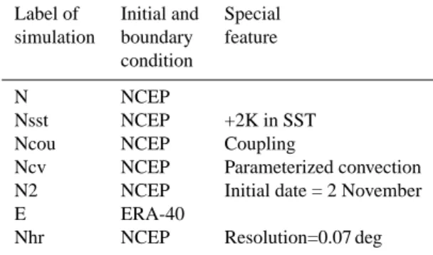
Table 1. Characteristics of the simulations mentioned in the text
and labels used to denote them.
Label of Initial and Special simulation boundary feature
condition
N NCEP
Nsst NCEP +2K in SST Ncou NCEP Coupling
Ncv NCEP Parameterized convection N2 NCEP Initial date = 2 November E ERA-40
Nhr NCEP Resolution=0.07 deg
energy balance equation along the ray followed by the wave component while approaching the shore. The source func-tion that describes the local rate of energy variafunc-tion in the shallow water is different from that used by WAM, because the overall effect of the deep water source function is on the scale of the near shore zone much smaller than the interac-tion with the bottom that produces the breaking of the wave, whose expression is based on the study of Battjes and Janssen (1978).
3.7 Simulations
Seven simulations have been carried out. A summary of their characteristics and the labels used for denoting them can be found in Table 1.
Six simulations have been performed with the MIAO model. Only one high resolution simulation, labelled “Nhr”, was carried out using BOLAM, HYPSE and WAM sepa-rately. Note that this allows to provide a high resolution forcing for the wave and ocean circulation models. Figure 2 shows the computational grids of the three modules in the MIAO model and those used for the high resolution atmo-spheric and marine simulations.
Within the MIAO model, BOLAM’s grid has a 0.27 deg resolution both in latitude and longitude in rotated coordi-nates, and 30 vertical levels. POM adopts a regular grid with 0.1 deg resolution, and 19 vertical levels. A 0.2 deg lat-lon resolution is used for WAM’s grid. Bathymetry for POM and WAM has been extracted from a global dataset at 1/12 deg resolution2.
The initialization of the three modules follows different procedures. For WAM, it is based on a wind-sea spectrum computed on the basis of the initial wind field. When it is used as a component of MIAO, the open boundary is lim-ited to the Gibraltar Strait and is ignored, while in the high resolution experiment it is in the southern part of the
Adri-2Data are available at http://topex.ucsd.edu/marine topo/mar
Fig. 2. Computational grids of the models used in this study. Large
dark gray area: BOLAM within MIAO. Smaller light gray area: BOLAM at high resolution. Large square box covering the whole Mediterranean: POM and WAM within MIAO. Smaller box cover-ing Italy: WAM high resolution. Smallest box: HYPSE (only points inside the Adriatic Sea are considered in the simulation).
atic basin. The initialization of POM is based on a previ-ous simulation initialized using climatological values from the Mediterranean Oceanographic DataBase 3. Initial and boundary conditions for the atmospheric model BOLAM are provided either by ERA-40 (simulation named “E”) or by NCEP re-analysis (all the other simulations with initial “N” in the label).
Integration begins on 1 November 00:00 UTC, except in the “N2” simulation, where it starts one day later, on 2 November 00:00 UTC.
The purpose of the various experiments can be understood, considering the “N” simulation as a reference. The “N” sim-ulations uses the fixed SST from NCEP re-analysis, it explic-itly describes convection, condensation and precipitation in case of convective instability, and computes the surface drag using the Charnock formula. With respect to it, the “N2” simulation is meant to test the effect of a different initial condition. In the “E” simulation the difference in the ini-tial condition is larger and also the boundary conditions are different, as they are extracted from a different analysis.
The effects of other model features have been studied. In the “Ncv” convective instability is parameterized: in this way the development of convection on unrealistic spatial scales, due to the coarse spatial resolution of the model, is inhib-ited. The “Ncou” simulation accounts for the feedback of the ocean circulation and the wave field on the air-sea fluxes, via the SST and the sea surface roughness, respectively: this is the only experiment where the two-way coupling is de-scribed. Therefore it shows the effect of different surface boundary conditions (the SST of the POM simulation is dif-ferent from that of the ERA-40 data) and of the increased
3http://modb.oce.ulg.ac.be
surface stress exerted by wind waves during the early stage of their growth. The “Nsst” simulation is identical to the “N” simulation, but the SST has been uniformly increased by 2 K over the whole Mediterranean basin, producing much stronger latent and sensible heat fluxes.
The ”Nhr” simulation provides information on the impor-tance of the resolution of the atmospheric model. In such simulation, the BOLAM model has been run alone, with a 0.07 deg resolution in longitude and latitude. In this case, a double nesting has been performed, as the imposed initial and boundary conditions for this simulation have been ob-tained from the “N” simulation. This simulation begins on 2 November 00:01 UTC. The computed high resolution atmo-spheric fields have been successively used to force the WAM and HYPSE models separately. In this experiment WAM uses a regular grid with 0.2 deg lat/lon resolution, as in the MIAO simulations. HYPSE has an orthogonal grid with a variable spatial resolution: the grid step has a minimum value of 0.03 deg in the northern Adriatic, and increases towards the border of the grid with a 1.01 scaling factor. This implies a higher resolution with respect to the simulation with the MIAO model. Finally, WAM and HYPSE’s high resolution results have been used to force the NSM model, in order to provide an estimate of the wave set-up.
This set of experiments is meant on one side to understand what are the model features important for the accurate sim-ulation of such intense events, on the other side to identify the aspects of the evolution of the extreme event which, be-ing common to all simulations, are a basic component of the disastrous event.
Only the four experiments which resulted to be the most significant (“E”, “N”, “Nsst” and “Nhr”) have been selected to show their results in the figures, for sake of clarity.
3.8 Data
In order to describe the sequence of events which character-ized the storm, several sources of data have been used.
Data provided by regional models simulations are needed to provide the details that cannot be obtained by the observa-tions or by the coarse resolution global re-analysis.
The CENFAM (“CEntro Nazionale di Fisica dell’Atmosfera e Meteorologia”) general documenta-tion on the meteorological situadocumenta-tion associated to this storm. The analysis is based on SLP, wind, precipitation, temperature and specific humidity data including both me-teorological stations, radiosoundings and the soundings of the radar located in the Roma Fiumicio Airport (CENFAM, 1967). This documentation includes the hand made analysis of the Italian Air Force Meteorological Service (IAFMS).
Surface atmospheric variables have been measured at 34 Italian stations: SLP and U10 have been sampled every 3 hours, while for precipitation the accumulated amount be-tween 06:00 UTC and 18:00 UTC of each day is available. Some of these stations are located in mountainous areas,
where precipitation fell in the form of snow: in these cases data are not reliable and have not been used in the analysis. Sea level data were provided by tide gauge data operated in Venice by the Italian Hydrographic and Mareographic Ser-vice4and by model simulations.
Surface and pressure level data used to obtain the initial and boundary conditions for the model simulations are provided by the ERA-40 and NCEP re-analysis. The ERA-40 re-analysis (Gibson et al., 1997) has a T159 spectral resolution (corresponding to about 130 km resolution) on the horizontal ad 60 vertical levels. The NCEP re-analysis (Kalnay et al., 1996) is performed with a T62 spectral model (correspond-ing to about 210 km resolution) with 28 vertical levels. Data from both dataset are available every 6 hours.
The extreme value analysis on the precipitation field, illus-trated in Sect. 6, has been performed using the synop-data of the meteorological stations, available for about 40 years for most of them.
4 The evolution of the storm
4.1 Synoptic evolution
The synoptic situation associated to the event can be appre-ciated, on the large scale, in Fig. 3, that shows the SLP (top panel) and the GPH500 (bottom panel) fields, according to the ERA-40 re-analysis, on 4 00:00 UTC, when the storm is entering its mature stage. The choice of ERA-40 rather than NCEP data is due to their higher resolution, and is justified by the fact that differences between the two re-analysis in the SLP field are not big, probably because of the data as-similation process (De Zolt et al., 2006). In the SLP maps, the cyclone associated to the storm which hit Italy is over the western Thyrrenian Sea. A second deeper and larger cy-clone located south of Iceland is connected to the first one through a low pressure area which covers all central Europe. The combination of the two pressure minima determines a flow of cold air directly from the polar regions to the west-ern Mediterranean and northwest-ern Africa, which is stronger at higher levels. Over the central Mediterranean, instead, a south-westerly flow brings warm and moist air towards cen-tral and eastern Europe. This intense meridional circulation determined a strong meridional transport of heat and mois-ture (Bert´o et al., 2005) and, as a consequence, a highly baro-clinic situation over the western Mediterranean Sea, respon-sible for the rapid intensification and strengthening of the cy-clone that hit Italy. Furthermore, the advection of the cold northern air over the Mediterranean region, where the sur-face temperature is anomalously high, determines a strong convective instability of the air mass over the Mediterranean sea, leading to intense updraft and the formation of
convec-4Magistrato alle Acque, ufficio idrografico e mareografico di
Venezia
Fig. 3. SLP (top panel) and GPH500 (bottom panel) in the
ERA-40 re-analysis, on 4 November 00:00 UTC, when the storm reached the mature stage. SLP values are in hPa. Contour line interval is every 5 hPa. Darker gray levels denote lower values. Levels from 1015 to 1035 hPa are denoted with black lines. GPH500 values are in gpm. Contour line interval is every 80 gpm. Darker gray levels denote lower values. Levels from 5600 to 5920 gpm are denoted with black lines.
tive systems evident in the meteorological radar soundings (CENFAM, 1967).
Cyclogenesis starts over the western Mediterranean. On 3 November 00:00 UTC, at the 500 hPa level, a trough lo-cated over north-western Europe, already present in the pre-vious days, develops a sharper feature on its western side which moves from France to the Mediterranean region, while a ridge over eastern Mediterranean and central-eastern Eu-rope becomes more and more intense, starting the intense meridional circulation.
On 4 00:00 UTC, the cyclone has rapidly strengthened and developed complex mesoscale structures, which cannot be appreciated in Fig. 3 owing to the coarse contour interval used, but are represented by the IAFMS analysis. The cen-tral area of the pressure minimum is elongated in the merid-ional direction. The axis of this structure corresponds to the
cold front which separates the cold northern air to the west from the warm African and Mediterranean air to the east. Several small size local minima have formed along the front and, even if some of them last just for a few hours, they act intensifying the local phenomena. The trajectory and the depth of three main local minima, here named “A”and “B”, according to the IAFMS analysis, are shown in Figs. 5 and 6. The detection and tracking of the cyclone centres has been performed with the procedure described in Lionello et al. (2002). The deep and persistent minimum “A” corre-sponds to the main cyclone, that on 3 00:00 UTC is located in the western Mediterranean, and follows a path characteristic of several cyclones that form in the North-Western Mediter-ranean Sea. A second minimum, labeled “B”, develops later, on 3 18:00 UTC, south of Sardinia, intensifies and moves northward. There is evidence of the presence of a third min-imum, named “C”, more shallow and located south of the Atlas mountains, in a region where cyclogenesis is more fre-quent in winter and spring. Its evolution cannot be followed in the IAFMS analysis, as its location is partially outside the meteorological charts, but its presence is shown by the NCEP and ERA-40 re-analysis.
The combination of the different minima determines an in-tense zonal pressure gradient over Italy and the Adriatic Sea, that is further reinforced by the presence of a large high pres-sure area above the Balkan peninsula (third and fourth panel of Fig. 4). According to the IAFMS hand made analysis, on 4 November 12:00 UTC, the value of such pressure difference over the Adriatic basin exceeds 18 hPa.
On 5 00:00 UTC, the deep Atlantic cyclone that on 4 00:00 UTC was located south of Iceland moves south-eastward towards north-western Europe: the trough visible in the 500 hPa maps moves north-eastward and, at the sur-face, the Mediterranean cyclone gradually dissolves, making phenomena cease over Italy.
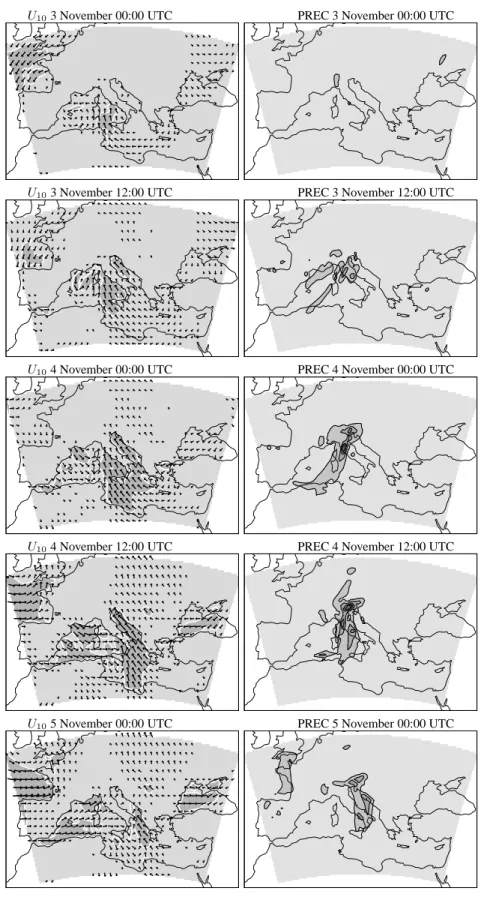
4.2 Winds, precipitation and surge
The zonally sharp and meridionally elongated SLP gradient, extending over Italy and the Adriatic basin, and the asso-ciated intense mass, heat and moisture transport are proba-bly the most peculiar characteristic of this event. The ra-diosoundings in north-eastern Italy (CENFAM, 1967) indi-cate that on 3 November 12:00 UTC the air was close to sat-uration (relative humidity was higher than 95%) in a layer 3 km high near the surface. The associated southerly sirocco wind was particularly strong in the northern Adriatic sea, where, channeled between Apennines and Dinaric Alps (Li-onello et al., 2003b), reached its maximum intensity on 4 November 12:00 UTC. No observations are available in the open sea: the estimate provided by the models is about 25 ms−1 for U10. At Venice airport, on the inland border of the venetian lagoon, the highest hourly recorded value is 19 ms−1 and it is likely lower than the value offshore. The
panels in the left column of Fig. 7 show the U10 evolution according to the “N” simulation.
The wind produced very high waves and storm surge in the northern Adriatic. No measurement is available for waves. The storm surge contribution was about 170 cm on the ba-sis of the observation in the Venice city centre, which corre-sponds to a return time of about 250 years. Luckily, the surge was an isolated event, which was not superimposed with a previous seiche and whose peak took place when the astro-nomical tide contribution was negligible and actually slightly negative. The time series of the surge observed at the coast of Venice is shown in Fig. 8. The pattern of this field, on 4 November 12:00 UTC, according to the “N” simulation (Fig. 9), shows that the sea surface level anomaly has the typical distribution caused by a sirocco storm, during which the action of the wind, blowing towards the Venetian coast, and of the SLP, lower in the northern than in the southern part of the basin, accumulate water at the shallow northern part of the Adriatic Sea. This evidence suggests that an im-portant role in the extreme impact of the event is played by the anomalously long fetch associated to the circulation, de-termined by the particular structure of the low pressure sys-tem, with several local minima, and by the high pressure over north-eastern Europe.
The orographic uplift of the warm and humid air trans-ported by the sirocco was the cause of the extreme precipita-tion that affected the northern Apennines, first, and the east-ern Alps, later. Actually, precipitation affected all the Italian peninsula, but was less intense in the southern regions.
Over the Thyrrenian Sea, the cold front to the west and the Apenines to the east forced the air flow towards the ridge on the border between Tuscany and the Po valley. As a con-sequence of the orographic uplift, intense precipitation fell on the western side of the mountain chain, particularly over the Arno’s and Ombrone’s basins. The further contribution of the convective precipitation, caused by the high vertical instability of the air over the Thyrrenian Sea, is highlighted by radar soundings (CENFAM, 1967), which show the pres-ence of several convective cells, some of them organized in a squall line, preceding the cold front.
On the eastern Alps the orographic precipitation was even more intense, because the air flow impinged the mountain chain frontally and the sirocco had a longer fetch over sea. The radiosoundings in Nort-Eastern Italy (CENFAM, 1967) show that, initially, the rise of the flow on the Alps was sheltered by eastern barrier winds (Malguzzi, 2006), blow-ing over the Po basin till 3 November 18:00 UTC: the rapid pressure decrease observed in this region on 3 November corresponds to the change in the circulation, when eastern winds cease and the onset of sirocco determines intense pre-cipitation all over the pre-alpine and alpine region of north-eastern Italy. This is confirmed by the rapid temperature and specific humidity increase that is shown by radiosoundings (CENFAM, 1967). The precipitation recorded at some me-teorological stations during the main part of the event (from
GPH500 3 November 00:00 UTC SLP 3 November 00:00 UTC
GPH500 3 November 12:00 UTC SLP 3 November 12:00 UTC
GPH500 4 November 00:00 UTC SLP 4 November 00:00 UTC
GPH500 4 November 12:00 UTC SLP 4 November 12:00 UTC
GPH500 5 November 00:00 UTC SLP 5 November 00:00 UTC
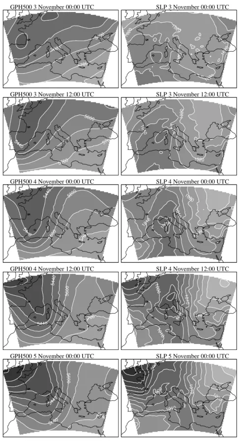
Fig. 4. Left column: GPH500. Panels show the results of the ”N” simulation at 12 hours intervals, from 3 to 5 November 00:00 UTC, from
top to bottom. Contour lines are every 80 gpm. Right column: as for left column, but for the SLP. Contour lines are every 5 hPa.
Fig. 4. Left column: GPH500. Panels show the results of the “N” simulation at 12 h intervals, from 3 to 5 November 00:00 UTC, from top
Obs E N Obs E N
Fig. 5. Trajectories of the low pressure centres in the simulations
and in the IAFMS hand made analysis. Some trajectories are in-terrupted, when the corresponding minimum is temporarily not de-tected in the SLP maps. No analysis data are available for the “C” minimum, since its location is partially outside the IAFMS meteo-rological charts. Labels “Obs”, “E”, “N” and the associated arrows indicate the position of the “A” and “B” minima on 4 November 00:00 UTC, according to the IAFSM charts, E and N simulations, respectively.
2 November 18:00 UTC to 5 06:00 UTC) is represented in Fig. 10 (middle panel), while the time series of the accumu-lated precipitation, averaged for north-eastern Italy and Tus-cany, is shown in Fig. 11 (the estimate is based on stations indicated in the figure).
Because of the high precipitation, all the rivers, whose catchment basins are on the alpine and pre-alpine chain and on the northern part of the Apennines, reached excep-tional levels, that determined the disastrous floods in Tuscany and north-eastern Italy. On this respect, the contribution of the meteorological situation of the months preceding the 4 November storm was important. In fact, during September and October 1966, widespread precipitation fell all over cen-tral and northern Italy. Daily precipitation values were high, even if not exceptional, but the duration of the rainy period was considerable. Locally, also numerous downpours took
Fig. 6. Time series of the “A” (top) and “B” (bottom) SLP minima
in the simulations and observations (values in hPa, Y-axis). Time in hours, from 3 November 00:00 UTC to 6 November 00:00 UTC is shown in the X-axis. As in Fig. 5, curves are interrupted when the corresponding minimum is temporarily not detected in the SLP maps.
place. This situation determined a reduction of the ground-water tables receptivity, so that at the beginning of Novem-ber many drainage basins were already full and not capable to absorb any more water (Gazzolo, 1969). Furthermore, the soil conditions became favorable to the landslides which took place as a consequence of the storm. In addition to that, over the central and eastern Alps the snow cover was significant, reaching values in excess of 100 cm in some areas. Its melt-ing, caused by the advection of warm air from the southern Mediterranean, further increased the river’s discharge.
5 Factors affecting the simulations and comparison with observations
5.1 Evolution of SLP minima
The evolution of the synoptic system responsible for the ex-treme event, according to the results of the “N” simulations, is illustrated in Fig. 4, where the GPH500 and SLP maps are
U103 November 00:00 UTC PREC 3 November 00:00 UTC
U103 November 12:00 UTC PREC 3 November 12:00 UTC
U104 November 00:00 UTC PREC 4 November 00:00 UTC
U104 November 12:00 UTC PREC 4 November 12:00 UTC
U105 November 00:00 UTC PREC 5 November 00:00 UTC
Fig. 7. Results of the N simulation, as in Fig. 4. Left column, U10wind field at 12 hour intervals: inside the darker area the wind speed exceeds the 10 ms−1value. Right column, accumulated precipitation (PREC) in the previous 12 hours: the 10, 40, 80, 120, 160 mm contour lines are marked.
Fig. 7. Results of the N simulation, as in Fig. 4. Left column, U10wind field at 12 hour intervals: inside the darker area the wind speed
exceeds the 10 ms−1value. Right column, accumulated precipitation (PREC) in the previous 12 h: the 10, 40, 80, 120, 160 mm contour lines are marked.
Fig. 8. Time series of SWH (top panel), in m, and storm surge
(bot-tom panel), in m, near the shore of Venice. The X-axis shows time, in hours from 3 November 00:00 UTC to 6 November 00:00 UTC.
shown. The trajectories and the time series of the main local minima are represented in Figs. 5 and 6. The “Ncv”, “Ncou” and “N2” simulations, very similar to “N”, are not shown.
The complex mesoscale structure of the perturbation, char-acterised by the presence of multiple minima, cannot be appreciated in Fig. 4 owing to the coarse contour interval used, but it is present in all simulations. Despite the differ-ences among experiments, the intense zonal pressure gradi-ent, which represents the most peculiar characteristic of the event is reproduced in all cases, and is even stronger than in the IAFMS analysis.
The main result is that the initial and boundary condi-tions play the most important role, so that all simulacondi-tions based on NCEP data are relatively similar, while the only one based on ERA-40 data exhibits a different behavior. In fact, in all experiments in which initial and boundary con-ditions are extracted from NCEP data, minimum “A” forms east of the Balearic islands, and then moves over the Gulf of Lions and North-Western Italy. These results are not con-firmed by IAFMS data, which show that actually
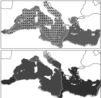
cycloge-Fig. 9. Top panel: SWH. Contour lines are marked every 1 m. When
the SWH is lower than 2 m, vectors are not drawn. Both panels refer to 4 November 12:00 UTC (about the peak of the storm), and to the N experiment. Bottom panel: sea level. Contour lines are marked every 20 cm. The darkest gray, covering most of the Eastern Mediterranean Sea, corresponds to values lower than, 0 cm.
nesis takes place over the Gulf of Valencia. The discrep-ancies with IAFSM data are bigger in the E simulation, in which the “A” minimum forms west of Corsica and quickly moves North, so that, on 4 November 00:00 UTC, while the E simulation shows a well developed minimum over southern Germany, in the IAFSM data and in the simulations whose initial and boundary conditions are extracted from NCEP re-analysis the minimum is over the Ligurian Sea. Moreover, the trajectory of “B” looks correct in all simulations but E, in which it forms later, over central Italy, and then, before reaching Northern Italy, it temporarily dissolves to appear again further north, missing the final position of the “B” min-imum in the IAFSM maps. Figure 6 (lower panel) shows that in all simulations whose initial and boundary conditions are extracted from NCEP re-analysis minimum ”B” deepens too much, if compared with the IAFMS analysis. Note that, even if from this figure the E simulation might seem fitting better the IAFSM data, it misplaces the location of the “B” minimum so that the agreement with IAFSM data is actu-ally much worse than in all the other simulations. Also the “A” SLP minimum is lower than what reported in the IAFMS meteorological charts for all simulations, but one should be aware that “A” was almost located over sea, where little ob-servations are generally available, and in this case the IAFMS analysis might be not that accurate. The different descrip-tion of the mesoscale structure of the cyclone in the “E”
Fig. 10. Top panel: distribution of the accumulated precipitation
according to the “N” simulation (the contour line interval is 50 mm). Middle panel: observed accumulated precipitation at stations used for model validation. Bottom panel: corresponding values in the “N” model simulation. In the latter two panels the size of circles is proportional to the observed value of accumulated precipitation. All panels consider the period from 2 November 18:00 UTC to 5 November 06:00 UTC. The two squared boxes show the region used for evaluating the “north-eastern Italy” and ”Tuscany” time series.
Northern-Eastern Italy
Tuscany
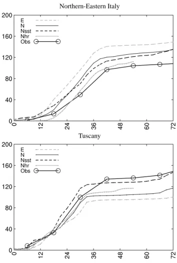
Fig. 11. Time series of accumulated precipitation averaged over the
“north-eastern Italy” (top panel) and “Tuscany” (bottom panel) ar-eas. The X-axis shows time, in hours, from 3 November 00:00 UTC to 6 November 00:00 UTC. The Y-axis shows precipitation, in mm.
simulation is determined by significant differences between the ERA-40 and NCEP re-analysis in the representation of the synoptic situation associated to the event (De Zolt et al., 2006).
The second factor, in order of importance, determining significant differences between experiments is resolution. The high resolution “Nhr” simulation produces a much ear-lier deepening and a too low value for minimum “A”, be-having differently from the rest of the simulations. This is consistent with its shorter time step and higher resolution, which allow to describe steeper pressure gradients. Further-more, this simulation does not develop the “C” minimum, whose presence is confirmed by the IAFMS analysis on 4 00:00 UTC, even if its trajectory is mostly out of the domain of these maps and it is not shown in Fig. 5.
The third factor is the higher SST. In the “Nsst” simulation minimum “B” forms earlier than in the other experiments, over the coast of Algeria, and it is deeper than in the IAFMS
Civitavecchia
Genoa
Ravena
Venice
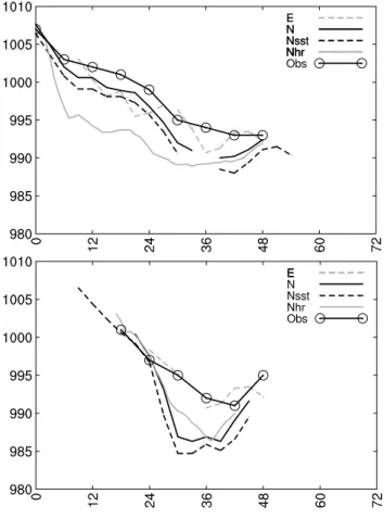
Fig. 12. Time series of SLP. The X-axis shows time, in hours from
3 November 00:00 UTC to 6 November 00:00 UTC. Y-axis shows SLP in hPa.
analysis and in the other experiments. This is consistent with a larger surface upward heat flux due to the higher tempera-ture of the sea surface. Also in this case the “C” minimum is not present.
Other model features such as to switch on the parameteri-zation of the convective precipitation (“Ncv”) and to change the initial condition (“N2”) have been tested (see Table 1) but their effect has been found small, that is their results are very similar to those of the “N” simulation. Also the coupling with the oceanographic models, performed in the “Ncou” simulation, does not produce significant differences from the results of the “N” simulation, where the coupling is switched off. Therefore, the two-way air-sea coupling is not an important feature for the simulation of this event.
The outlined characteristics of the simulations are substan-tially confirmed by the direct comparison with SLP time se-ries at several meteorological stations, as it is possible to see in Fig. 12. These plots also show that the “B” minimum moved faster in the simulations than in the observation and its passage was about 9 h earlier during the final part of the storm. The “Nhr” simulation presents a slightly better tim-ing.
5.2 Precipitation
The three precipitation maxima over north-eastern Italy, Tus-cany and Central Italy are reproduced by all simulations. Re-sults of the ”N” simulation are shown in Fig. 10 (top panel). The evolution of the precipitation, according to the same ex-periment, is shown in the right column of Fig. 7.
Figure 11 shows the time series of the precipitation accu-mulated in some meteorological stations located in northern Italy and Tuscany, where the highest values were recorded. For the two areas an average of the precipitation over 9 and 6 stations, respectively, has been made (see the boxes in Fig. 10). The comparison is done considering the model point nearest to the meteorological observation. The timing of the simulated precipitation agrees well with observations in the two regions, where, according to the observations, it started on 3 06:00 UTC and stopped on 4 18:00 UTC. The sampling time of the observations is not frequent enough to show that in Tuscany phenomena ceased some hours earlier than in Northern Italy, but this is reproduced by the simula-tions.
In Northern Italy precipitation is overestimated by all the simulations. The “E” simulation produces the highest values, while the “Nhr” better fits the observations.
Instead, in Tuscany precipitation is underestimated by all simulations. The higher precipitation of the “Nsst” simula-tion in this region is consistent with a large moisture contrast due to more evaporation over the Mediterranean. The “Nhr” simulation looks like being the best at reproducing precipita-tion, though it underestimates it in the last hours of 4 Novem-ber. This is consistent with the better representation of the orography, which is important for this event in which
precip-itation was mainly of orographic type. The parameterization of convective instability, performed in the ”Ncv” experiment, determines significant changes in the precipitation field only over Tuscany (not shown). In this region values are higher in the N case, where convective instability is explicitly com-puted, probably because of the development of convection on non realistic spatial scales, due to the too coarse resolution of the model (De Zolt et al., 2006).
The stations used to compute the time series in Fig. 11 are not fully representative of the total amount of precipitation. In fact, precipitation was much higher in north-eastern Italy than in Tuscany (CENFAM, 1967), which is reproduced by the precipitation maps in the simulations.
5.3 Surge and waves
The surge on the north-eastern Italian coast is produced by the combined effect of the atmospheric pressure gradient along the Adriatic basin and of the wind stress in the cross-shore direction. As the pressure difference along the Adri-atic basin reaches a maximum value of about 18 hPa in the IAFMS analysis, and up to 24 hPa in the model simulations, the inverse barometric effect accounts for about 20 cm surge. Therefore, in this case, as it is usual, the wind stress is the main responsible for the intensity of the surge. Figure 7 shows that the surface wind field presents the typical charac-teristics of a sirocco event, but with a particularly long fetch extending to northern Africa.
Time series of the sea elevation show that the surge event presents a simple signal both in model simulations and in observations (Fig. 8). Before the event the sea level has been flat for at least two days, so that there was no interaction of the storm surge with previous seiches and after the surge peak a sequence regular seiches was triggered. The wrong timing of the surge peak (occurring at 36 h from the beginning of the simulation) corresponds to the wrong timing of the SLP minimum (Fig. 12, fourth panel) and of the wind speed peak (Fig. 13, fourth panel). Consequently, the following seiche (occurring at 60 h) also presents a delay if compared with observations.
The time error is smaller for the “Nhr” simulation, which also better reproduces the peak value of the surge and the following seiches. This corresponds to a significantly better reproduction of the wind field, both on the timing of the peak and on the previous behavior. In all simulations, in Venice, the duration of the high wind period is too long, as observa-tions show a more sharply peaked event of the wind records (Fig. 13, fourth panel). This prolonged high wind period is simulated by the “Nhr” in the stations located on the eastern Adriatic coast, and is actually confirmed by the observations (Fig. 13, second and third panel). Probably, the simulated wind at the Venetian coast is not always well reproduced, due to the difficulty of representing the turbulent dynamics of the near-shore zone and of locating exactly the coastline, but its reconstruction in the open sea might be better in the
Civitavecchia
Bari
Falconara
Venice
Fig. 13. Time series of surface wind speed. The X-axis shows time,
in hours from 3 November 00:00 UTC to 6 November 00:00 UTC. Y-axis shows U10in ms−1.
Fig. 14. Time series of wave set-up (black continuous line, in cm)
computed by the NSM model, storm surge (continuous gray line, in cm) computed by the HYPSE model and SWH (black dashed line, in m×10−1) computed by the WAM high resolution simula-tion near the shore of Venice. The X-axis shows time, in hours from 3 November 00:00 UTC to 6 November 00:00 UTC.
high resolution simulation. Note that only the “E” simulation presents a severe underestimate of the surge peak.
The complex dynamics of the nearshore zone, where the wave set-up contribution to the sea elevation must be taken into account, cannot be simulated by the POM and HYPSE models. The NSM model described in Sect. 3 has been used to evaluate the wave set-up. The model has been forced with the surge computed by the HYPSE simulation and with the SWH reproduced by the WAM high resolution simulation. In Fig. 14 the simulated wave set-up, the surge and the SWH time series are compared. The maximum wave set-up near the coast is 30 cm and is reached on 4 November 11:00 UTC, one hour before the surge peak. The sum of surge and set-up reaches the maximum value of 191 cm on 4 November 12:00 UTC. This simulation suggests that the wave set-up ef-fect on the coastal defences was negligible if compared to that of the surge and of the waves.
The SWH time series at Venice (Fig. 8, upper panel) and Pescara, show a peaked event, during which the SWH in-creases towards north. No observation is available for val-idating these results. The 6 m SWH value simulated in the northern Adriatic is compatible with the extreme situation which took place at the Venetian littoral where waves were overriding and disrupting the coastal defenses with unprece-dented strength. However, at the coast waves were clearly depth limited on the shallow gently sloping sea bottom and an evaluation of SWH offshore is not possible on the basis of their height at the coast.
6 Discussion
6.1 Modeling issues
The largest effect on the model simulation is determined by the use of initial and boundary conditions extracted from dif-ferent re-analysis. This implies that the “E” simulation pro-duces the weaker cyclone, and misses a major feature, that is the passage of the “B” minimum over central and northern Italy. This causes a severe underestimate of the peak level of the storm surge and large errors in precipitation, which is underestimated over Tuscany and overestimated over the north-eastern Alps. These results are determined by the dif-ferent representation of the synoptic situation in the ERA-40 and NCEP re-analysis, evident from the potential vorticity fields both in the initial condition and in the following days (De Zolt et al., 2006).
The model resolution is the second factor as importance. In the “Nhr” high resolution simulation the behavior and tim-ing of the “B” SLP minimum, and, consequently, of the surge peak, is reproduced better than in all other simulations. Fur-thermore, it produces the best results, on average, for the pre-cipitation field. On the other side, the deepening of the “A” minimum takes place too early.
The specification of SST comes as third factor. The “Nsst” simulation, with a high SST (likely unrealistic), determines a too intense cyclone, but a satisfactory reproduction of precip-itation, wind and surge level. This poses the question if the October SST in the Western Mediterranean Sea is correctly represented in the in the re-analysis. On the other side the SLP minimum is too low in the ”Nsst” simulation. Therefore the improvement in the precipitation points to a problem of the model boundary layer representation, which is compen-sated by an overestimate of the intensity of the cyclone.
Other factors are less important. The parameterization of the convective precipitation (“Ncv”), the two-way coupling between atmosphere and ocean (“Ncou”) and the choice of a different initial condition extracted from the same NCEP re-analysis (“N2”) have a small effect.
In conclusion, the initial and boundary conditions, the spa-tial resolution and the SST are the most important factors. The improvement in the results determined by increasing the model resolution is lower than it could be expected. Actu-ally the “N” simulation performs reasonably well for most variables, and it shows that the MIAO model would be able to simulate accurately the meteorological and oceanic evolu-tion of the storm.
6.2 Exceptionality of the event and factors at play
The exceptionality of the event studied is evident from the huge damages it produced all over central and northern Italy. Several factors contribute in determining its gravity: the precipitation fallen during the storm and in the preceding
months, the rivers overflow, landslides, the high waves and storm surge.
A GEV (Generalized Extreme Value) analysis of the an-nual precipitation maxima has been performed on the data recorded at the meteorological stations indicated in Fig. 15, where the return times associated to the precipitation accu-mulated in 12 h (upper panel) and in 24 h (lower panel) are shown. It is evident that precipitation was extreme in few stations, and that return times are larger for the 24 than for the 12 h accumulated precipitation. In Volterra and Grosseto (Tuscany), and in Bolzano, Dobbiaco and Tarvisio (North-eastern Alps), return times exceed 50 years for the 24 h accu-mulation period. Nevertheless, these return times are lower than one would expect from the damages produced by the storm and from the levels reached by the rivers. Actually, the contribution from other factors than the precipitation during the event have to be considered.
The sea surge in the northern Adriatic was more extreme than the precipitation over north-eastern Italy, the return time associated to its peak value being higher than 250 years. The exceptionality of the surge is itself an assessment of the strength and spatial extension of the wind field, for which the extreme value analysis has not been carried out.
Note, that the value of the SLP minimum, though low, can-not explain the extreme impact and high damage produced by the storm. An approximate evaluation based on previous analysis (Lionello et al, 2002) suggests that cyclones with this depth of the minimum take place more than once every year. It is evident that the exceptionality of the phenomena associated to the storm has been determined by the synoptic and mesoscale structure of the cyclone, characterized by the presence of multiple pressure minima and of an intense zonal pressure gradient, and not by the pressure minimum itself. No climatological assessment of the frequency of systems with multiple SLP minima and the presence of local minima both in the western Mediterranean and on northern Africa is available. However, the analysis of the precipitation and storm surge extremes suggests that the feature that produced the extreme surge has to be characterized by a comparably low probability of occurrence.
7 Conclusions
The reconstruction of the meteorological and marine aspects of the event does not leave major open issues. It is sensitive to some factors, like initial and boundary conditions, reso-lution and SST, but, though the agreement between models and observations is not complete and no model simulation is fully satisfactory, the sequence of events can be clearly as-sessed. The storm was caused by a cyclone, which formed on the western Mediterranean. Interaction with mesoscale oro-graphic feature and local processes (latent heat release) pro-duced a peculiar situation with several combined SLP min-ima. The long fetch of the sirocco wind combined with the
Fig. 15. Return times associated to the precipitation accumulated in
12 h (upper panel) and in 24 h (lower panel). The size of the circles is representative of the return time, as shown in the labels.
intense SLP gradient caused the storm surge in the northern Adriatic Sea. Strong advection of moist air from the Central Mediterranean Sea produced intense and persistent precipi-tation over central Italy and the eastern Alps. Not all aspects of the event reached extreme intensity, and those that were extreme were such at different levels. This reconstruction is consistent with the damage produced by the storm.
This study does not provide a conclusive evidence on the factors responsible for the extreme character of the event. There are four firm points for the evaluation of the intensity of the event. The cyclone was not remarkably deep as the damages that were produced. The storm surge in the north-ern Adriatic Sea was extreme, with a return time of about 250 years or even more. Precipitation was extreme over the north-eastern Alps and in Tuscany, where return times ex-ceed 50 years in some stations, but it is possible that the anal-ysis of a dataset coming from a more dense station network would give higher return times for the stations located over
the mountainous areas. The runoff values for the Adige and Tagliamento rivers are likely centennial.
Other factors can explain the higher relative intensity of river runoff compared to that of precipitation. The abun-dant precipitation of the previous months and the melting of snow, caused by the sudden temperature rise associated to the south-easterly sirocco wind, are also accounted respon-sible for the high value of return times. Furthermore, it is important to consider that, because of the persistent precipi-tation of the previous months, the water storage capacity of the soil was pretty low. The extreme intensity of the isolated surge event (there was no interaction with previous surge or high astronomical tide) clearly supports the extreme inten-sity of the sirocco wind and its long fetch. This in turn is consistent with the intense precipitation associated with the orographic uplift of large amount of moist air, whose pres-ence is confirmed over large parts of the Mediterranean Sea by the meteorological analysis during the event. Other stud-ies have shown the presence of a significant contribution to the moisture flux coming from Northern Africa and the East-ern Atlantic (Bert´o et al., 2005): it would be interesting to analyse the dynamic role of this flux. This might help in un-derstanding the causes of the exceptionality of the storm.
On one hand this study shows that the simulation of the meteorological event would have been possible with reason-able accuracy, considering present-day model capabilities. At the same time it shows that it would have been difficult to predict the extent of the damage from the value reached by single meteorological variables during the storm and that several factors have to be accounted for. The SLP minimum alone was not an indication of the extreme intensity of the event. The anomalous fetch of the sirocco wind, determined by the particular structure of the SLP field, was more cru-cial than the wind speed itself for the extreme intensity of the surge and for the northward transport of warm and humid air from the southern Mediterranean. The floods and landslides would, certainly, at least, have been favored by critical soil condition and snow melting in the Alps. Therefore a precise monitoring of the territory would have been needed for pre-dicting the damage and the use of a chain of impact models driven by meteorological fields and computing waves, surge, soil conditions and river runoff. These arguments stress the importance of an integrated model system for predicting and managing extreme events.
Acknowledgements. NCEP reanalysis data are provided by
the NOA CIRES Climate Diagnostic Center, Boulder, Col-orado, USA, and have been downloaded from their web site at http://www.cdc.noaa.gov. ERA-40 data are retrieved from the ECMWF MARS archive. The authors are grateful for permission by Aeronautica Militare Italiana to use this link.
Edited by: A. Barros Reviewed by: three referees
References
APAT (Agenzia per la protezione dell’ambiente e per i servizi tec-nici); Agenzie Regionali e delle Provincie Autonome per la Pro-tezione Ambientale ; SISTAN, Sistema Statistico Nazionale: An-nuario dei dati ambientali, edizione 2004, XXII, pp. 1192, Roma: APAT, c2005 : I.G.E.R
Battjes, J. A., and Janssen, J. P. F. M.: Energy loss and set-up due to breaking of random waves, Proc. 16th Int. Conf. on Coastal Eng., ASCE, 569–587, 1978.
Bendini, C.: Bacini della Toscana, in: L’evento alluvionale del novembre 1966, Roma, Istituto poligrafico dello stato, Libreria, pp. 41–85, 1969.
Bert´o, A., Buzzi, A., and Zardi, D.: A warm conveyor belt mech-anism accompanying extreme precipitation events over north-eastern Italy, Proceedings of the 28th ICAM, The annual Scien-tific MAP Meeting, 2005, Zadar, Extended Abstracts, Hrv. Me-teorol. Casopis (Croatian Meteorological Journal), 40, 338–341, 2005.
Blumberg, A. F. and Mellor, G. L.: A description of a 3-dimensional coastal ocean circulation model, edited by: Heaps, N. S., AGU, Washington D.C., 1–16, 1987.
Buzzi, A., Fantini, M., Malguzzi, P., and Nerozzi, F.: Validation of a limited area model in cases of mediterranean cyclogenesis: surface fields and precipitation scores, Meteorol. Atmos. Phys., 53, 137–153, 1994.
Canestrelli, P., Mandich, M., Pirazzoli, P. A., Tomasin, A.: Wind, depression and seiches: tidal perturbations in Venice (1951– 2000), Citt`a di Venezia, Centro Previsioni e Segnalazioni Maree, Comune di Venezia, 1–104, 2001.
Commissione interministeriale per lo studio della sistemazione idraulica e della difesa del suolo: L’evento alluvionale del novembre 1966. Roma, Istituto poligrafico dello stato, 193 pp., 1969.
CENFAM (Consiglio Nazionale delle Ricerche, CEntro Nazionale di Fisica dell’Atmosfera e Meteorologia) and Ministero della Difesa-Aeronautica, ITAV, Servizio Meteorologico. Prima docu-mentazione generale della situazione meteorologica relativa alla grande alluvione del novembre 1966, Parte II., Roma, CENFAM, 1967.
De Zolt, S., Lionello, P., Malguzzi, P., Nuhu, A., and Tomasin, A.: The effect of the boundary conditions on the simulation of the 4 November 1966 storm over Italy, Adv. Geosci., 7, 199–204, 2006,
http://www.adv-geosci.net/7/199/2006/.
Dorigo, L.: Bacini del Veneto, in: L’evento alluvionale del novembre 1966, Roma, Istituto poligrafico dello stato, Libreria, pp. 133–165, 1969.
Fea, G.: Sintesi descrittiva degli eventi meteorologici legati alle grandi alluvioni verificatesi nell’Italia centro-settentrionale tra il 3 ed il 5 novembre 1966, in: L’evento alluvionale del novembre 1966, Roma, Istituto poligrafico dello stato, Libreria, pp. 7–25, 1969.
Frassetto, R.: Altimetria del centro storico di Venezia, Bollettino di Geofisica Teorica ed Applicata, vol. XIII, n. 71, 1976.
Gazzolo, T.: Notizie di carattere generale sugli eventi idrologici, in: L’evento alluvionale del novembre 1966, Roma, Istituto poligrafico dello stato, Libreria, pp. 27–39, 1969.
Gibson, J. K., Kallberg, P., Uppala, S., Noumura, A., Hernandez, A., and Serrano, E.: ERA Description. ECMWF Re-Analysis