HAL Id: hal-00604013
https://hal.archives-ouvertes.fr/hal-00604013
Submitted on 14 Jan 2021
HAL is a multi-disciplinary open access archive for the deposit and dissemination of
sci-L’archive ouverte pluridisciplinaire HAL, est destinée au dépôt et à la diffusion de documents
Rosetta-Alice observations of exospheric hydrogen and
oxygen on Mars
Paul D. Feldman, Andrew J. Steffl, Joel Wm. Parker, Michael F. A’Hearn,
Jean-Loup Bertaux, S. Alan Stern, Harold A. Weaver, David C. Slater,
Maarten Versteeg, Henry B. Throop, et al.
To cite this version:
Paul D. Feldman, Andrew J. Steffl, Joel Wm. Parker, Michael F. A’Hearn, Jean-Loup Bertaux, et al.. Rosetta-Alice observations of exospheric hydrogen and oxygen on Mars. Icarus, Elsevier, 2011, 214 (2), pp.394-399. �10.1016/j.icarus.2011.06.013�. �hal-00604013�
arXiv:1106.3926v1 [astro-ph.EP] 20 Jun 2011
Rosetta-Alice Observations of Exospheric Hydrogen
and Oxygen on Mars
Paul D. Feldmana,∗, Andrew J. Stefflb, Joel Wm. Parkerb, Michael F. A’Hearnc, Jean-Loup Bertauxd, S. Alan Sternb, Harold A. Weavere, David C. Slaterf, Maarten Versteegf, Henry B. Throopb, Nathaniel J. Cunninghamg, Lori M.
Feagac
aJohns Hopkins University, Department of Physics and Astronomy, 3100 N. Charles Street,
Baltimore, MD 21218 USA
bSouthwest Research Institute, Department of Space Studies, Suite 300, 1050 Walnut Street,
Boulder CO 80302-5150 USA
cDepartment of Astronomy, University of Maryland, College Park MD 20742-2421 USA dLATMOS, CNRS/UVSQ/IPSL, 11 Boulevard d’Alembert, 78280 Guyancourt, France eJohns Hopkins University Applied Physics Laboratory, Space Department, 11100 Johns
Hopkins Road, Laurel, MD 20723-6099 USA
fSouthwest Research Institute, P. O. Drawer 28510, San Antonio TX 78228-0510 USA gPhysics Department, Nebraska Wesleyan University, Lincoln, NE 68504-2794 USA
Abstract
The European Space Agency’s Rosetta spacecraft, en route to a 2014 en-counter with comet 67P/Churyumov-Gerasimenko, made a gravity assist swing-by of Mars on 25 February 2007, closest approach being at 01:54 UT. The Alice instrument on board Rosetta, a lightweight far-ultraviolet imaging spectrograph optimized for in situ cometary spectroscopy in the 750–2000 ˚A spectral band, was used to study the daytime Mars upper atmosphere including emissions from exo-spheric hydrogen and oxygen. Offset pointing, obtained five hours before closest approach, enabled us to detect and map the HI Lyman-αand Lyman-βemissions from exospheric hydrogen out beyond 30,000 km from the planet’s center. These data are fit with a Chamberlain exospheric model from which we derive the hy-drogen density at the 200 km exobase and the H escape flux. The results are comparable to those found from the the Ultraviolet Spectrometer experiment on the Mariner 6 and 7 fly-bys of Mars in 1969. Atomic oxygen emission at 1304 ˚A is detected at altitudes of 400 to 1000 km above the limb during limb scans shortly after closest approach. However, the derived oxygen scale height is not consistent with recent models of oxygen escape based on the production of suprathermal
oxygen atoms by the dissociative recombination of O+2.
Keywords: Mars, Mars atmosphere, Atmospheres, evolution
1. Introduction
The extended atomic hydrogen corona of Mars was first detected by the ultra-violet spectrometer experiments on the Mariner 6 and 7 spacecraft that measured resonantly scattered solar Lyman-αradiation (Barth et al., 1971) to a planetocen-tric distance of 24,000 km. This was followed by a similar experiment on the or-biting Mariner 9 mission (Barth et al., 1972). Anderson and Hord (1971), using radiative transfer theory, analyzed the early data to derive a hydrogen escape rate, which they found to be compatible with the water photodissociation rate at Mars. Barth et al. (1972) recognized that the apparently constant H escape rate derived from Mariner 6, 7, and 9, if extended backward over geological time scales, would result in an oxygen abundance in the lower atmosphere several orders of magni-tude larger than observed. McElroy (1972) suggested that dissociative recombi-nation of O+2, the dominant ion in the atmosphere, would produce oxygen atoms with sufficient energy to escape. However, since the energetic oxygen atoms are mostly produced below the exobase, determination of the escaping fraction re-quires detailed modeling, represented by the recent work of Lammer et al. (2003), Fox and Ha´c (2009), Shematovich et al. (2007), Valeille et al. (2009, 2010), and others. Barth et al. (1971) also reported observations of OI λ1304 emission up to 700 km. These data, together with those from Mariner 9, were interpreted by Strickland et al. (1973) in terms of a cool, optically thick oxygen exosphere. Since then, the only measurement of exospheric oxygen on Mars is from the SPICAM instrument on Mars Express (Chaufray et al., 2009), but those data extended only up to 400 km where radiative transfer effects in the OIλ1304 multiplet are sig-nificant and the evidence for a hot component of O atoms was inconclusive.
Until recently there have also been no additional measurements of the ex-tended hydrogen atmosphere on Mars. Chaufray et al. (2008), again with SPI-CAM, have measured HILyman-αemission at 1216 ˚A, but only up to 4,000 km. Again, they find that a two temperature H exosphere is possible, although the
result is inconclusive. Clarke et al. (2009) also suggest a two-component H distri-bution from monochromatic Lyman-αimages of Mars showing the H corona out to 4 Mars radii (RM) taken by the Solar Blind Channel of the Advanced Camera for Surveys on HST. Radiative transfer modeling is necessary to extract densities from both of these data sets. Clarke et al. also noted a variation in the Lyman-α brightness over a period of two months which they ascribe to a seasonal variation in the H2O loss rate.
We report here on observations of both the extended hydrogen and oxygen coronae of Mars made with the Alice far-ultraviolet imaging spectrograph (Stern et al., 2007) on Rosetta during the spacecraft’s gravity assist swing-by of Mars on 25 February 2007. Offset exposures enabled us to detect and map the HI Lyman-α and Lyman-βemissions to beyond 30,000 km from the planet’s center. Moreover, except near the planet’s limb, the Lyman-βemission is optically thin, allowing us to use a spherical Chamberlain model to determine the temperature and density of H at the exobase without the need for radiative transfer modeling. From limb pointings at spacecraft distances closer to the planet, oxygen emission above the exobase is detected, allowing us to constrain the density of hot oxygen without the need for radiative transfer modeling. These data can be used to derive atomic escape rates and address the question of stoichiometric loss of water vapor from Mars.
2. Observations
Rosetta approached Mars from the day side making its closest approach (CA)
at 01:54 UT on 25 February 2007 at an altitude of 250 km. In order to satisfy the scientific goals of the various remote sensing instruments (see, e.g., Coradini, 2010), the common instrument boresight was programmed for a number of fixed pointings towards both the sunlit and dark hemispheres of Mars and offset from Mars, as well as raster scans across the sunlit limb. Due to operational constraints, observations were not possible during the immediate CA period. The pointings of interest in this paper (denoted by the operational designation ALxx) were AL03 pre-CA, centered on the sunlit disk, AL10E, offset pointings centered 2.5◦ and 7.5◦from Mars along the equator, and AL11B, scans across the illuminated cres-cent post-CA. Observation start times and geometry parameters are given in Ta-ble 1. At the time of closest approach, Mars was 1.445 AU from the Sun and the areocentric longitude, Ls, was 189.9◦. Solar activity was very low for an extended time, including when Earth faced the same solar longitude 9 days earlier, with
Alice is a lightweight, low-power, imaging spectrograph optimized for in situ cometary far-ultraviolet (FUV) spectroscopy. It is designed to obtain spatially-resolved spectra in the 750-2000 ˚A spectral band with a spectral resolution be-tween 8 and and 12 ˚A for extended sources that fill its field-of-view. The slit is in the shape of a dog bone, 5.5◦long, with a width of 0.05◦in the central 2.0◦while the ends are 0.10◦wide. Each spatial pixel along the slit is 0.30◦. Alice employs an off-axis telescope feeding a 0.15-m normal incidence Rowland circle spectro-graph with a concave holospectro-graphic reflection grating. The imaging microchannel plate detector utilizes dual solar-blind opaque photocathodes (KBr and CsI) and employs a two-dimensional delay-line readout. Details of the instrument are given by Stern et al. (2007).
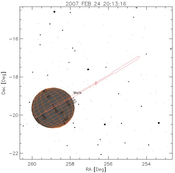
The Alice slit geometry, illustrating the shape of the multi-segment slit, is shown in Fig. 1 for the first pre-CA offset pointing of 2.5◦. The second offset moved the slit an additional 5.0◦away from Mars parallel to the Martian equator. Except near the limb, the only features seen in the offset spectra are HI
Lyman-α and Lyman-β, and these data are used to extract the spatial profiles of these emissions.
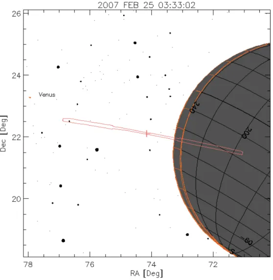
A similar diagram for the post-CA limb scans, beginning 25 February 2007 at UT 03:33:02, is shown in Fig. 2. At this time each spatial pixel projected to 280 km in altitude but as Rosetta receded from Mars the projected size of each pixel increased. The scan slowly shifted the boresight ∼250 km towards Mars over a 15-minute period. This is illustrated in Fig. 3. Because of the scanning motion, these spectra were acquired in “pixel-list” mode, that is the position of each photon count is recorded together with a time tag so that spectra could be reconstructed with the motion accounted for. Because the Rosetta-Alice instru-ment has only a single data buffer, the data gaps seen in Fig. 3 result from the time required to read out the buffer to the spacecraft. The typical time to fill the buffer was 30 s, so in practice we accumulated individual spectra corresponding to ∼30 s integrations. Even so, to detect OI emission at high altitudes, we need to co-add multiple spectra, as described below.
3. Data Analysis
3.1. Calibration
During the gravity assist swing-bys of both Mars and the Earth, the Rosetta instruments were powered on and operated primarily to provide flight
verifica-exercise the full range of instrument parameters that could be adjusted by remote command in flight in order to optimize the signal-to-noise performance of the instrument. For the Mars swing-by, the detector high voltage level was set at –3.8 kV. Subsequent operations and analysis showed the optimum setting to be –3.9 kV and all observations beginning in the fall of 2007 were made at that volt-age. Nevertheless, by comparison of stellar standards at different voltages (and at different times), we are able to transfer the current absolute flux calibration to the epoch of the Mars swing-by and this is incorporated into the current version of the data pipeline (version 3) with which all of the data have since been processed. The data used in this study are publicly available, both from NASA’s Planetary Data System (http://pdssbn.astro.umd.edu/) and ESA’s Planetary Science Archive (http://www.rssd.esa.int/?project=PSA).
To derive spatial profiles of the observed emissions requires an accurate flat-field calibration. This poses a rather acute problem for Lyman-α at 1216 ˚A be-cause the instrument was designed for this wavelength to fall in the gap between the KBr and CsI photocathode coatings. The intent was to utilize the low detection efficiency of the bare microchannel plate to compensate for the very high expected Lyman-αphoton flux from the comet. However, because of a slight misalignment in the coating edges, the Lyman-α sensitivity varies by a factor of two along the portion of the detector that is mapped onto the sky. In contrast, at Lyman-βthe variation across the slit is ∼1.4. There is also a ±20% odd-even detector row effect that is accentuated at the lower detector high voltage of –3.8 kV.
Fortuitously, following the Mars encounter, Rosetta-Alice was pointed to-wards Jupiter and recorded many hours of spectra in support of the New
Hori-zons fly-by of Jupiter in February 2007. These observations were made with the
same instrument parameters used for the Mars observations. Since, from the or-bit of Mars the Jovian system only filled a single row of the detector, high S/N measurements of detector flat-fields at Lyman-αand Lyman-βwere obtained, to-gether with a measure of grating scattered Lyman-αas a function of detector row. An added bonus is that since Jupiter was only 20◦ away on the sky from the coordinates of the offset pointing, these observations provided a measure of the interplanetary Lyman-αand Lyman-βbackground for the Mars observations. We used a co-added accumulation of 630,000 s of data obtained between 1 March and 10 March 2007 to derive the flat-fields used in the analysis described below.
3.2. Mars dayglow spectrum
We briefly discuss the dayglow spectrum of Mars, obtained under AL03 pre-CA. It consisted of four exposures, each of 1028 seconds. A composite of the
five central rows of the sum of four exposures is shown in Fig. 4. The viewing parameters are given in Table 1. At the start of the sequence, the angular diameter of Mars was 1.62◦ so that the five central rows of the detector were uniformly filled with the illuminated Martian disk. For comparison with previous work, we also show the Mars full disk spectrum recorded by the Hopkins Ultraviolet Tele-scope (HUT) on board the Space Shuttle in March 1995 (a full solar cycle earlier) (Feldman et al., 2000), convolved to the spectral resolution of Alice. At the time, Mars was 1.666 AU from the Sun, Ls was 70.5◦, and F10.7 was ≈75. The HUT spectrum is multiplied by a factor of 0.80 to match the brightness observed by Alice, and this is quite good agreement considering the Alice calibration uncer-tainty and the fact that the HUT spectrum measured the integrated disk brightness, not just a central stripe of the disk. The comparison also serves to validate the wavelength calibration and provides a reference spectrum with which to compare the exospheric spectra obtained in AL10E and AL11B. As noted by Barth et al. (1972) and Leblanc et al. (2006), with the exception of the HILyman series and OIλ1304, Mars’ dayglow emissions, principally CO and CI, are confined to alti-tudes below ∼200 km.
3.3. Offset exposures
The two offset exposures were taken immediately following the full disk spec-tra as Rosetta approached Mars. HILyman-βwas detected along the full length of the Alice slit for both offsets. Because the slit is segmented, for each row along the slit the observed Lyman-β signal was fit to a gaussian profile superimposed on a grating-scattered background that was fit to a second-order polynomial. The flux was then obtained by integrating under the gaussian and then correcting for the detector flat-field that was derived from subsequent Jupiter observations as de-scribed in Section 3.1. The result is shown as a histogram in Fig. 5. The errors shown are statistical in the count rate. The Lyman-α profile is similarly derived except that the detector background, due to dark counts, was negligible, and is shown in Fig. 6. The shape of this profile is very similar to the slant intensity profiles derived from the Mariner 6 and 7 fly-bys by Barth et al. (1971), although lower in absolute brightness as the Mariner fly-bys occurred at a time of high solar activity. Neither Fig. 5 nor Fig. 6 have had the interplanetary background subtracted as did the plots of Barth et al. The model fits to the data are discussed below in Section 4.1.
3.4. Limb scan spectra
From the data acquired in pixel list mode during the limb scans schematically illustrated in Fig. 3, we can extract a spectrum spanning a given time interval. However, because the line-of-sight of the spectrogram was changing its position above the limb with time, it is necessary to balance the motion with the need for a sufficiently long integration time to obtain an adequate signal-to-noise ratio for weak emission features. At the same time, we need to avoid contamination of the spectrum by thermospheric emissions. This was done by co-adding the photon counts from the first four exposures for row 14; the first 12 exposures for row 15; and the last 14 exposures for rows 16 and 17. This results in an altitude weighted average with a trapezoidal shape of ≈320 km centered at 420, 665, 910, and 1240 km, respectively for rows 14 to 17, respectively.
Examples of extracted spectra for rows 15 and 16 are shown in Fig. 7. Note that only HIand OI emissions are detected. A possible feature at 1657 ˚A in the row 15 spectrum that could be a signature of escaping carbon atoms (Fox and Ha´c, 1999; Cipriani et al., 2007), is most likely an instrumental artifact as no emission at this wavelength appears in the row 14 spectrum. The background is due to grating scattered Lyman-α, which is variable from row to row. Also, the spectra have not been corrected for the odd-even row variation noted in Section 3.1 which is estimated to be ∼25% for Lyman-βand ∼10% for OIλ1304, based on the disk observations discussed in Section 3.2.
4. Discussion
4.1. Exospheric hydrogen model
For the analysis of the Lyman-β profile we follow the same procedure as Anderson and Hord (1971), using the exospheric model of Chamberlain (1963) but ignoring satellite orbits, as they can be excluded by the observed Lyman-β brightness near 30,000 km planetocentric distance. For solar minimum conditions we take the exobase to be at 200 km and the exobase temperature, Te, to be 200 K (Krasnopolsky, 2002; Fox and Ha´c, 2009), leaving the hydrogen density at this level as a variable. We assume that Lyman-βis optically thin and calculate a flu-orescence efficiency (g-factor) of 3.9 × 10⁻⁶ photons s−1 atom−1 at 1 AU using a solar minimum line profile and flux from Lemaire et al. (2002). The interplane-tary Lyman-βbackground is fixed at 1.0 rayleigh based on the subsequent Jupiter observations that were used to derive the detector flat-field at 1026 ˚A (see Sec-tion 3.1). All fluxes are referenced to row 15 which is the nominal Alice boresight and which is used for almost all of the stellar calibration measurements.
The result is shown by the solid curve in Fig. 5. The derived H density at 200 km is 2.5 × 105 cm−3and the escape flux is 7.8 × 107cm−2 s−1. The model atmosphere is given in Table 2. Optical depth unity along the line-of-sight is at
∼5,000 km projected planetocentric distance. From the radiative transfer model
of Anderson and Hord (1971), applied to the Mariner Lyman-α data, we expect the single scattering intensity to be about a factor of two higher than the radiative transfer corrected intensity at this optical depth, and this is consistent with the data shown in Fig. 5. Anderson and Hord, for their solar maximum observations, assuming Te=350 K at an exobase altitude of 250 km, found an H density and escape flux of 3.0 × 104 cm−3 and 1.8 × 108 cm−2 s−1, respectively. Fig. 5 also shows a model for 260 K (dashed line), which, normalized at 30,000 km, provides what superficially appears to be a better fit to the observed profile. While it is difficult to choose between the models for planetocentric distances greater than 10,000 km, the absence of a strong optical depth effect in the latter suggests that the lower temperature model, corresponding to a typical exospheric temperature at solar minimum, is probably correct. For 260 K, the H density and escape flux are 9.0 × 104cm−3 and 1.34 × 108cm−2s−1, respectively.
The same models, applied to Lyman-αusing a Lyman-α/Lyman-βratio of 250 derived from the IPM measurements, are shown in Fig. 6. The agreement is excel-lent and the deviation from the optically thin emission is consistent with an optical depth along the line-of-sight of 1 at 10,000 km planetocentric distance. There is no apparent need for a suprathermal H component as suggested by Chaufray et al. (2008) and Clarke et al. (2009).
An interesting measurement of exospheric Lyman-αemission from Mars
Ex-press has recently been reported by Galli et al. (2006). They found that the Neutral
Particle Detector of the ASPERA-3 experiment was sensitive to Lyman-αphotons and measured a signal, attributed to exospheric hydrogen, out to a tangent height of 7,250 km above the Martian limb. Considering their large measurement uncer-tainties that include calibration, statistics, pointing, and background subtraction, their measured emission profile is in general accord with the Alice data shown in Fig. 6. However, they interpret this profile in terms of an optically thin resonance scattering model and derive an apparent temperature > 600K. As noted above, we find that the Lyman-αemission is optically thick below 10,000 km planetocentric distance (∼6,600 km above the limb), which leads to a flatter spatial distribution and consequently the appearance of a higher than actual exospheric temperature.
4.2. Two-component oxygen model
For oxygen we use a two-component model, again taking for the cold com-ponent, Te, to be 200 K, and an oxygen density at 200 km of 3.0 × 107 cm−3 (Fox and Ha´c, 2009). The curve in Fig. 8 represents an added hot component of 1200 K with an oxygen density at 200 km of 1.0 × 105 cm−3 (see Table 2). The density decrease with altitude is considerably faster than the predictions of recent exospheric models of Chaufray et al. (2009) and Valeille et al. (2010) based on a hot atomic O source due to dissociative recombination of O+2, and which are necessary to support a stoichiometric escape of water vapor from the atmosphere of Mars. However, it has been noted that such inferences from a single viewing geometry during a period of low solar activity can be misleading as this mecha-nism is quite sensitive to solar activity and is dependent on solar zenith angle at the observation point.
Nevertheless, the present observations raise concern about some of the as-sumptions and physical parameters used in the recent modeling of oxygen escape from Mars. Fox and Ha´c (2009), in their comparison of exobase and Monte Carlo models, summarize the literature on modeling efforts from the past few decades and conclude that “efforts to balance the escape rates in the stoichiometric propor-tion of water are premature.” Fox and Ha´c focus on a comparison of escape rates and therefore do not compute the oxygen density profiles from their models. Such calculation is warranted by the present data which would allow for a determination of the line-of-sight column densities appropriate to the Alice observations.
Similar questions arise in the analogous modeling of the hot oxygen environ-ment around Venus (Gr¨oller et al., 2010). Bovino et al. (2011) discuss the need for accurate data on energy transfer collisions between hot oxygen atoms and the neutral atmosphere (they are mainly interested in helium) which is at the core of the escape models. Finally, we note that Simon et al. (2009) point out that an ad-ditional constraint on the models might be provided by SPICAM measurements of the forbidden OIλ2972 (1S –3P) line, which is produced by both photodisso-ciation of CO2and by dissociative recombination of O+2.
5. Conclusion
The Rosetta swing-by of Mars on 25 February 2007, provided the first spec-troscopic observations of exospheric hydrogen and oxygen on Mars from outside Mars’ atmosphere since the Mariner 6 and 7 fly-bys in 1969. The spatial distribu-tion of HILyman-αout to beyond 30,000 km from the planet’s center is similar to
that found from Mariner 6 and 7. A Chamberlain model, with current solar mini-mum model values of exospheric temperature of 200 K and an exobase altitude of 200 km, provides a good fit to the observed Lyman-βprofile, although the data do not exclude temperatures up to ∼260 K. A suprathermal component, suggested by several authors, is not needed to match the data. The hydrogen escape flux derived from the 200 K model, 7.8 × 107cm−2s−1, is comparable to that derived from the earlier measurements. The distribution of atomic oxygen, derived from 1304 ˚A emission observed to altitudes of 1000 km above the limb, is not consistent with recent models of oxygen escape based on the production of suprathermal oxygen atoms by dissociative recombination of O+2.
Acknowledgments
We thank the ESA Rosetta Science Operations Centre (RSOC) and Mission Operations Center (RMOC) teams for their expert and dedicated help in planning and executing the Alice observations of Mars. We thank Darrell Strobel for help-ful discussions. The Alice team acknowledges continuing support from NASA’s Jet Propulsion Laboratory through contract 1336850 to the Southwest Research Institute. The work at Johns Hopkins University was supported by a sub-contract from Southwest Research Institute.
References
Anderson, Jr., D.E., Hord, C.W., 1971. Mariner 6 and 7 ultraviolet spectrometer experiment: Analysis of hydrogen Lyman-alpha data. J. Geophys. Res. 76, 6666–6673.
Barth, C.A., Hord, C.W., Pearce, J.B., Kelly, K.K., Anderson, G.P., Stewart, A.I., 1971. Mariner 6 and 7 ultraviolet spectrometer experiment: Upper atmosphere data. J. Geophys. Res. 76, 2213–2227.
Barth, C.A., Stewart, A.I., Hord, C.W., Lane, A.L., 1972. Mariner 9 Ultravi-olet Spectrometer Experiment: Mars Airglow Spectroscopy and Variations in Lyman Alpha. Icarus 17, 457–468.
Bovino, S., Zhang, P., Gianturco, F.A., Dalgarno, A., Kharchenko, V., 2011. En-ergy transfer in O collisions with He isotopes and Helium escape from Mars. Geophys. Res. Lett. 38, 2203.
Chamberlain, J.W., 1963. Planetary coronae and atmospheric evaporation. Planet. Space Sci. 11, 901–960.
Chaufray, J.Y., Bertaux, J.L., Leblanc, F., Qu´emerais, E., 2008. Observation of the hydrogen corona with SPICAM on Mars Express. Icarus 195, 598–613. Chaufray, J.Y., Leblanc, F., Qu´emerais, E., Bertaux, J.L., 2009. Martian
oxy-gen density at the exobase deduced from O I 130.4-nm observations by Spec-troscopy for the Investigation of the Characteristics of the Atmosphere of Mars on Mars Express. J. Geophys. Res. 114, 2006.
Cipriani, F., Leblanc, F., Berthelier, J.J., 2007. Martian corona: Nonthermal sources of hot heavy species. J. Geophys. Res. 112, 7001.
Clarke, J.T., Bertaux, J., Chaufray, J., Gladstone, R., Quemerais, E., Wilson, J.K., 2009. HST Observations Of The Extended Hydrogen Corona Of Mars. Bull. Am. Astron. Soc. 41, 49.11 (abstract).
Coradini, A., et al., 2010. Martian atmosphere as observed by VIRTIS-M on Rosetta spacecraft. J. Geophys. Res. 115, 4004.
Feldman, P.D., Burgh, E.B., Durrance, S.T., Davidsen, A.F., 2000. Far-Ultraviolet Spectroscopy of Venus and Mars at 4 ˚A Resolution with the Hopkins Ultraviolet Telescope on Astro-2. Astrophys. J. 538, 395–400.
Fox, J.L., Ha´c, A., 1999. Velocity distributions of C atoms in CO+
dissocia-tive recombination: Implications for photochemical escape of C from Mars. J. Geophys. Res. 104, 24729–24738.
Fox, J.L., Ha´c, A.B., 2009. Photochemical escape of oxygen from Mars: A com-parison of the exobase approximation to a Monte Carlo method. Icarus 204, 527–544.
Galli, A., Wurz, P., Lammer, H., Lichtenegger, H.I.M., Lundin, R., Barabash, S., Grigoriev, A., Holmstr¨om, M., Gunell, H., 2006. The Hydrogen Exospheric Density Profile Measured with ASPERA-3/NPD. Space Sci. Rev. 126, 447– 467.
Gr¨oller, H., Shematovich, V.I., Lichtenegger, H.I.M., Lammer, H., Pfleger, M., Kulikov, Y., Macher, W., Amerstorfer, U.V., Biernat, H.K., 2010. Venus’ atomic hot oxygen environment. J. Geophys. Res. 115, 12017.
Krasnopolsky, V.A., 2002. Mars’ upper atmosphere and ionosphere at low, medium, and high solar activities: Implications for evolution of water. J. Geo-phys. Res. 107, 5128.
Lammer, H., Lichtenegger, H.I.M., Kolb, C., Ribas, I., Guinan, E.F., Abart, R., Bauer, S.J., 2003. Loss of water from Mars:Implications for the oxidation of the soil. Icarus 165, 9–25.
Leblanc, F., Chaufray, J.Y., Lilensten, J., Witasse, O., Bertaux, J., 2006. Mar-tian dayglow as seen by the SPICAM UV spectrograph on Mars Express. J. Geophys. Res. 111, E09S11.
Lemaire, P., Emerich, C., Vial, J.C., Curdt, W., Sch¨uhle, U., Wilhelm, K., 2002. Variation of the full Sun hydrogen Lyman-α and β profiles with the activity cycle, in: Wilson, A. (Ed.), From Solar Min to Max: Half a Solar Cycle with SOHO, Noordwijk: ESA SP-508. pp. 219–222.
McElroy, M.B., 1972. Mars: An Evolving Atmosphere. Science 175, 443–445. Shematovich, V.I., Tsvetkov, G.A., Krestyanikova, M.A., Marov, M.Y., 2007.
Stochastic models of hot planetary and satellite coronas: Total water loss in the Martian atmosphere. Solar System Res. 41, 103–108.
Simon, C., Witasse, O., Leblanc, F., Gronoff, G., Bertaux, J., 2009. Dayglow on Mars: Kinetic modelling with SPICAM UV limb data. Planet. Space Sci. 57, 1008–1021.
Stern, S.A., Slater, D.C., Scherrer, J., Stone, J., Versteeg, M., A’Hearn, M.F., Bertaux, J.L., Feldman, P.D., Festou, M.C., Parker, J.W., Siegmund, O.H.W., 2007. Alice: The Rosetta Ultraviolet Imaging Spectrograph. Space Sci. Rev. 128, 507–527.
Strickland, D.J., Stewart, A.I., Barth, C.A., Hord, C.W., Lane, A.L., 1973. Mariner 9 ultraviolet spectrometer experiment: Mars atomic oxygen 1304- ˚A emission. J. Geophys. Res. 78, 4547–4559.
Valeille, A., Combi, M.R., Tenishev, V., Bougher, S.W., Nagy, A.F., 2010. A study of suprathermal oxygen atoms in Mars upper thermosphere and exosphere over the range of limiting conditions. Icarus 206, 18–27.
Valeille, A., Tenishev, V., Bougher, S.W., Combi, M.R., Nagy, A.F., 2009. Three-dimensional study of Mars upper thermosphere/ionosphere and hot oxygen corona: 1. General description and results at equinox for solar low conditions. J. Geophys. Res. 114, 11005.
Table 1: Observation Parameters.
Observation ID AL03 AL10E AL11B
Start time (UT 2007) 24 Feb 18:28:14 24 Feb 20:13:14 25 Feb 03:33:02 Boresight pointing disk center offset 2.5◦, 7.5◦W E limb scan
Distance to Marsa(km) 239,800 184,200 51,600
Solar elongationa 164.3◦ 164.0◦ 24.3◦
Longitude of tangent point at limbb 213.9◦ 149.7◦ 263.6◦ Latitude of tangent point at limbb –1.8◦ –4.1◦ –26.5◦ Solar zenith angle at tangent pointb 15.7◦ 74.3◦ 67.9◦
Data mode Histogram Histogram Pixel list
Total integration time (s) 4112 483 + 1028 aAt start of observation.
Table 2: Model Atmosphere Densities. Altitude H O (cold) O (hot)
(km) (cm−3) (cm−3) (cm−3) 200 2.50 × 10⁵ 3.00 × 10⁷ 1.00 × 10⁵ 400 1.69 × 10⁵ 6.86 × 10⁴ 3.70 × 10⁴ 600 1.19 × 10⁵ 288.0 1.49 × 10⁴ 800 8.61 × 10⁴ 2.04 6520. 1000 6.42 × 10⁴ 0.023 3080. 1200 4.90 × 10⁴ 3.7 × 10⁻⁴ 1550. 1400 3.82 × 10⁴ 830. 1600 3.03 × 10⁴ 1800 2.44 × 10⁴ 2000 1.99 × 10⁴ 4000 4330. 6000 1590. 8000 757. 10000 422. 15000 144. 20000 67.5 25000 37.5 30000 23.2 35000 15.5
FIGURE CAPTIONS
Fig. 1. Projection of the Alice slit on the sky with the common boresight offset 2.5◦ from the center of Mars along the equator. Orange grid lines outline the illuminated region of the disk. The shape of the multi-segment slit is shown. Detector row numbers increase from left to right with the boresight (+) in row 15. Fig. 2. Projection of the Alice slit on Mars at the beginning of the limb scans following closest approach. Orange grid lines outline the illuminated crescent of the disk. Detector row numbers increase from right to left with the boresight (+) in row 15.
Fig. 3. Projection of individual rows of the Alice slit above the Mars limb dur-ing the slow limb scan followdur-ing closest approach. Initially, each spatial pixel projected to 280 km in altitude but as Rosetta receded from Mars the projected size of each pixel increased. The scan also slowly shifted the boresight ∼250 km towards Mars over a 15-minute period. The cross-hatched areas indicate the time during which photon events were accumulated while the horizontal lines show the times for which photon events were co-added for each row.
Fig. 4. The dayglow spectrum of Mars is a composite of the five central rows of four exposures, each of 1028 seconds. For comparison with previous work, we also show the Mars full disk spectrum recorded by the Hopkins Ultraviolet Telescope (HUT) at 4 ˚A spectral resolution in March 1995 (a full solar cycle earlier) (Feldman et al., 2000), convolved to the spectral resolution of Alice and multiplied by a factor of 0.8.
Fig. 5. HI Lyman-βwas detected along the full length of the Alice slit for both offsets. The data are shown as a histogram: black, 2.5◦ offset, red: 7.5◦ offset. The errors shown are statistical in the count rate. Optically thin Chamberlain models without satellite orbits for T=200 K (solid line) and 260 K (dashed line) are shown, superimposed on a 1 rayleigh interplanetary background. The radius of Mars is indicated.
Fig. 6. Same as Fig. 5 for HILyman-α. The shape of this profile is very similar to the slant intensity profiles derived from the Mariner 6 and 7 fly-bys by Barth et al. (1971), although lower in absolute brightness as the Mariner fly-bys occurred at a time of high solar activity. The same models are shown, superimposed on an
interplanetary background of 250 rayleighs.
Fig. 7. Extracted limb scan spectra. For row 15 (top), the photon counts from the first 12 exposures (376 s, see Fig. 3) were co-added. For row 16 (bottom), the last 14 exposures (476 s) were co-added. Only HIand OIemissions are detected. Fig. 8. Extracted OIλ1304 brightness from rows 14–17 as a function of altitude above the Martian limb. The vertical bars illustrate the extent of the trapezoidal altitude weighting function for each row while the horizontal bars are the statis-tical uncertainty in the count rate. The two-component oxygen model shown is described in the text.
Figure 1: Projection of the Alice slit on the sky with the common boresight offset 2.5◦from the center of Mars along the equator. Orange grid lines outline the illuminated region of the disk. The shape of the multi-segment slit is shown. Detector row numbers increase from left to right with the boresight (+) in row 15.
Figure 2: Projection of the Alice slit on Mars at the beginning of the limb scans following closest approach. Orange grid lines outline the illuminated crescent of the disk. Detector row numbers increase from right to left with the boresight (+) in row 15.
30 35 40 45 50 Time from 2007−02−25T03:00 (minutes)
−200 0 200 400 600 800 1000 1200
Distance above Mars limb (km)
Row 14
Row 13 Row 15 Row 16
Figure 3: Projection of individual rows of the Alice slit above the Mars limb during the slow limb scan following closest approach. Initially, each spatial pixel projected to 280 km in altitude but as Rosetta receded from Mars the projected size of each pixel increased. The scan also slowly shifted the boresight ∼250 km towards Mars over a 15-minute period. The cross-hatched areas indicate the time during which photon events were accumulated while the horizontal lines show the times for which photon events were co-added for each row.
800 1000 1200 1400 1600 1800 Wavelength (Å) 0 2 4 6 8 10 Brightness (Rayleighs Å −1 ) OII Lyγ Lyβ+OI OI OI ArI CI CI CO CO OI OI CO A−X
Figure 4: The dayglow spectrum of Mars is a composite of the five central rows of four exposures, each of 1028 seconds. For comparison with previous work, we also show the Mars full disk spectrum recorded by the Hopkins Ultraviolet Telescope (HUT) at 4 ˚A spectral resolution in March 1995 (a full solar cycle earlier) (Feldman et al., 2000), convolved to the spectral resolution of Alice and multiplied by a factor of 0.8.
10 Planetocentric Distance (x103 km) 1 10 Brightness (rayleighs) RMars Lyman−β
Figure 5: HILyman-βwas detected along the full length of the Alice slit for both offsets. The data are shown as a histogram: black, 2.5◦offset, red: 7.5◦offset. The errors shown are statistical in the count rate. Optically thin Chamberlain models without satellite orbits for T=200 K (solid line) and 260 K (dashed line) are shown, superimposed on a 1 rayleigh interplanetary background. The radius of Mars is indicated.
10 Planetocentric Distance (x103 km) 100 1000 10000 Brightness (rayleighs) RMars Lyman−α
Figure 6: Same as Fig. 5 for HILyman-α. The shape of this profile is very similar to the slant intensity profiles derived from the Mariner 6 and 7 fly-bys by Barth et al. (1971), although lower in absolute brightness as the Mariner fly-bys occurred at a time of high solar activity. The same models are shown, superimposed on an interplanetary background of 250 rayleighs.
1000 1200 1400 1600 Wavelength (Å) 0 1 2 3 4 5 Brightness (Rayleighs Å −1 ) row 15 Lyγ Lyβ OI 1000 1200 1400 1600 Wavelength (Å) 0 1 2 3 4 5 Brightness (Rayleighs Å −1 ) row 16 Lyγ Lyβ OI
1 10 100 1000 OI 1304 Brightness (Rayleighs) 200 400 600 800 1000 1200 1400 Altitude (km)
Figure 8: Extracted OI λ1304 brightness from rows 14–17 as a function of altitude above the Martian limb. The vertical bars illustrate the extent of the trapezoidal altitude weighting function for each row while the horizontal bars are the statistical uncertainty in the count rate. The two-component oxygen model shown is described in the text.