Upper-stratospheric ozone trends 1979-1998

HAL Id: hal-01638361

https://hal.archives-ouvertes.fr/hal-01638361

Submitted on 10 Jan 2020

HAL is a multi-disciplinary open access

archive for the deposit and dissemination of

sci-entific research documents, whether they are

pub-lished or not. The documents may come from

teaching and research institutions in France or

abroad, or from public or private research centers.

L’archive ouverte pluridisciplinaire HAL, est

destinée au dépôt et à la diffusion de documents

scientifiques de niveau recherche, publiés ou non,

émanant des établissements d’enseignement et de

recherche français ou étrangers, des laboratoires

publics ou privés.

Upper-stratospheric ozone trends 1979-1998

M. J. Newchurch, Lane Bishop, Derek Cunnold, Lawrence E. Flynn, Sophie

Godin, Stacey Hollandsworth Frith, Lon Hood, Alvin J. Miller, Sam Oltmans,

William Randel, et al.

To cite this version:

M. J. Newchurch, Lane Bishop, Derek Cunnold, Lawrence E. Flynn, Sophie Godin, et al..

Upper-stratospheric ozone trends 1979-1998. Journal of Geophysical Research: Atmospheres, American

Geophysical Union, 2000, 105 (D11), pp.14625 - 14636. �10.1029/2000JD900037�. �hal-01638361�

JOURNAL OF GEOPHYSICAL RESEARCH, VOL. 105, NO. Dll, PAGES 14,625-14,636, JUNE 16, 2000

Upper-stratospheric ozone trends 1979-1998

M. J. Newchurch,

•'2

Lane

Bishop,

3 Derek

Cunnold,

4 Lawrence

E. Flynn,

s Sophie

Godin,

6

Stacey

Hollandsworth

Frith,

7 Lon Hood,

a Alvin J. Miller,

9 Sam

Oltmans,

•ø

William

Randel,

• Gregory

Reinsel,

•2 Richard

Stolarski,

7 Ray

Wang,

4 and

Eun-Su

Yang•,

Joseph

M. Zawodny

•3

Abstract. Extensive

analyses

of ozone observations

between 1978 and 1998 measured

by Dobson

Umkehr, Stratospheric

Aerosol and Gas Experiment (SAGE) I and II, and Solar Backscattered

Ultraviolet (SBUV) and (SBUV)/2 indicate

continued

significant

ozone decline throughout

the

extratropical

upper stratosphere

from 30-45 km altitude. The maximum annual linear decline of

-0.8+0.2

% yr-•(2c•)

occurs

at 40 km and

is well described

in terms

of a linear

decline

modulated

by the 11-year

solar

variation.

The

minimum

decline

of-0.1+0.1%

yr-•(2c•)

occurs

at 25 km in

midlatitudes,

with remarkable

symmetry

between

the Northern and Southern

Hemispheres

at 40

km altitude.

Midlatitude upper-stratospheric

zonal trends

exhibit significant

seasonal

variation

(+30% in the Northern Hemisphere,

+40% in the Southern

Hemisphere)

with the most negative

trends

of-1.2% yr

-• occurring

in the winter.

Significant

seasonal

trends

of-0.7 to-0.9% yr -• occur

at 40 km in the tropics between

April and September.

Subjecting

the statistical

models used to cal-

culate the ozone trends to intercomparison

tests on a variety of common data sets yields results

that indicate the standard

deviation between trends estimated

by 10 different statistical

models is

less

than

0.1%

yr -• in the annual-mean

trend

for SAGE

data

and

less

than

0.2%

yr -• in the most

demanding

conditions

(seasons

with irregular, sparse

data) [World Meteorological Organization

(IfMO), 1998]. These consistent

trend results

between statistical

models together

with extensive

consistency

between

the independent

measurement-system

trend observations

by Dobson Umkehr,

SAGE I and II, and SBUV and SBUV/2 provide a high degree of confidence

in the accuracy

of the

declining ozone amounts

reported

here. Additional details of ozone trend results

from 1978 to

1996 (2 years shorter

than reported

here) along with lower-stratospheric

and tropospheric

ozone

trends,

extensive

intercomparisons

to assess

relative instrument

drifts, and retrieval algorithm de-

tails are given by tfMO [1998].

1. Introduction

stratosphere

the primary

mechanism

by which

CFCs

affect

ozone

is through gas-phase reactions involving chlorine radicals. Ozone

Substances of anthropogenic origin, such as chlorofluorocar-

changes in this region of the atmosphere provide a test of our un-

bons

(CFCs)and

bromine-containing

organic

volatile

compounds,

derstanding

of these

gas-phase

reactions.

Previous

studies

of

cause

stratospheric

ozone

depletion

[WMO,

1999].

In the

upper

stratospheric

ozone

trends

[WMO,

1995;

DeLuisi

et al., 1994;

•Department of Atmospheric Science, University of Alabama in Huntsville.

2Also at National Center for Atmospheric Research, Boulder, Colorado.

3Allied Signal Corporation, Buffalo, New York.

4School of Earth and Atmospheric Sciences, Georgia Institute of Tech- nology, Atlanta.

5NOAA/National Environmental Satellite Data and Information Serv-

ice, Silver Spring, Maryland.

6Service d'Aeronomie, Paris, France.

?NASA/Goddard Space Flight Center/Laboratory for Atmospheres,

Greenbelt, Maryland.

8Lunar and Planetary Laboratory, University of Arizona, Tucson. 9NOAA/National Weather Service/Climate Prediction Center, Camp

Springs, Maryland.

•øNOAA/Climate Monitoring and Diagnostics Laboratory, Boulder, Colorado.

•National Center for Atmospheric Research, Boulder, Colorado. •2Statistics Department, University of Wisconsin, Madison. •3NASA/Langley Research Center, Hampton, Virginia.

Copyright 2000 by the American Geophysical Union.

Paper number 2000JD900037. 0148-0227/00/2000JD900037509.00

McPeters et al., 1994; Reinsel et al., 1994; Rusch et al., 1994;

Miller et al., 1995, 1996] are summarized by Harris et al. [ 1997].

These studies found that ozone amounts from approximately 1979

to 1991

declined

at the rate of 0.5-1.0%

yr -• in northern

midlati-

tudes in the altitude region of maximum active chlorine (35-45 km). Those trend estimates were reasonably consistent in the three

measurement systems: Dobson Umkehr, Stratospheric Aerosol and Gas Experiment (SAGE) I/II, and Solar Backscattered Ultra- violet (SBUV). As previously noted by Hood et al. [1993] using NIMBUS-7 SBUV observations, the altitude-latitude structure and the seasonal structure of the measured ozone trends provide ex- cellent tests of our theoretical understanding of chlorine-catalyzed ozone destruction [Solomon and Garcia, 1984; Kaye and Rood,

1989] and the measured latitudinal distribution of C10 [Aellig et al., 1996; Waters et al., 1996]. Subsequent analyses of SAGE I/II trends through the same period employing an altitude correction for the SAGE I observations [ Wang et al., 1996] reconciled differ-

ences between SAGE I/II and SBUV trends that had been present

in the tropical lower stratosphere. Subsequent analysis of com-

bined SBUV and SBUV/2 (SBUV(/2)) trends [Hollandsworth et al., 1995], extended through 1994, did not substantially change that general agreement. These upper-stratospheric trends exhibited

latitudinal and seasonal variations such that the trends were more

14,626 NEWCHURCH ET AL.: UPPER-STRATOSPHERIC OZONE TRENDS 1979-1998

negative in the winter and spring seasons at high latitudes. The trends in the tropical latitudes are less negative throughout the stratosphere and exhibit little seasonal or altitudinal variation. At somewhat lower altitudes (10-20 hPa,-•30 kin), these three sys- tems, in addition to ozonesonde observations, concurred in finding

a statistically

insignificant

ozone

loss

of about-0.2

to -0.4%

yr

'•

over the 1979-1991 period.

The deduced trends in ozone concentration are in general agreement with the latitude and altitude characteristics of theoreti- cal predictions [e.g., Chandra et al., 1995; Jackman et al., 1996] that implicate halogen-induced ozone destruction; however, the magnitude of the model predictions has been somewhat larger than observed trends. These models also significantly overpredict the C10 amounts in the upper stratosphere, leading to overpredic- tions of ozone destruction. Recent laboratory measurements [Lip- son et al., 1997] determine that a minor channel of the reaction OH + C10 produces HC1, effectively reducing the C10/HC1 model excess. Including the HC1 branch in model chemistry brings the model ozone-trend predictions in line with observed trends [WMO, 1999]. However, the expected ozone recovery could be delayed if the current halogen growth continues into the next dec- ade [Fraser et al., 1999] or interactions between greenhouse-gas

increases and radiation slow dynamic transport of tropical air to higher latitudes and increase polar stratospheric cloud formation

due to lower temperatures [Shindell et al., 1998]. Then these lower

ozone columns will continue to affect surface UVB radiation

[Madronich et al., 1998].

Satellite-based instruments provide superior spatial coverage of

Earth compared to surface-based Dobson instruments; however,

the Dobson records extend many years prior to the satellite rec-

ords, and these instruments are routinely calibrated. The various

satellite instruments have different individual characteristics with

respect to long-term calibration stability, global coverage, vertical resolution, and sensitivity to contamination by stratospheric aero- sol. The solar-occultation instruments, SAGE I (which operated from 1979 to 1981) and SAGE II (1984 to present), employ at-

mospheric limb extinction at several wavelengths during sunrise

and sunset events. They have good long-term stability because

they are able to reference their atmospheric measurements to the

exoatmospheric sun before sunset and after sunrise for each verti- cal-profile measurement. Their vertical resolution is the best of all

satellite techniques (of the order of 1 km). However, their spatial coverage is relatively poor because of the requirement of an or- bital solar sunrise or sunset. Limb viewing in the visible/near- infrared is also subject to contamination by volcanic aerosols in the observation slant column, thereby making the ozone measure-

ments below-•20 km questionable [CunnoM et al., 2000b]. The

nadir-viewing backscatter ultraviolet (BUV) type instruments

SBUV (1978-1990) and SBUV/2 (1989-1994), which we denote as SBUV(/2) when referring to both instruments as a series from

1978-1994), have good global coverage for ozone profiles above

-•25 km but are subject to calibration uncertainties and the possi- bility of long-term drift and have relatively coarse vertical resolu-

tion. Aerosol contamination is a problem for these instruments

immediately following a major volcanic eruption.

The overall purpose of this paper is to extend by 2 years and to provide additional interpretation of the salient results of the analy- ses of WMO [ 1998], which reported extensive details on the in-

strument characteristics, relative instrument drifts, and trends in

both the stratosphere and troposphere. In addition to extending the analyzed time period, we also reanalyze the Dobson Umkehr rec- ord in a more consistent manner between two independent groups and provide significantly more information on the adequacy of the model fits to the Umkehr, SAGE I/II, and SBUV(/2) data series. Cunnold et al. [2000a] report on the uncertainties in these upper- stratospheric trends. Cunnold et al. [2000b] report trends in the lower stratosphere. Logan et al. [ 1999] report the tropospheric and

lower-stratospheric trends derived from ozonesonde observations. Randel et al. [1999] report the overview of trends and compari- sons at all altitudes.

Section 2 compares the results of the statistical trend models employed for the calculations. Section 3 presents the vertical pro- files of ozone trends in the upper stratosphere (20-50 km). The conclusions appear in section 4.

2. Statistical Models

A wide variety of statistical models has been used to derive trends in stratospheric ozone and to determine the effects on ozone of other variables such as the solar cycle and the quasi-biennial oscillation (QBO). The 1988 Trends Assessment [WMO, 1989, chapter 2] briefly intercompares results from a few of these statis-

tical models. While variations in the statistical model or in the an-

cillary variables (solar, QBO, nuclear effect, etc.) had relatively

minor effects on the calculated ozone trends, at least for total ozone, questions continue to arise as to how much of the differ-

ence in the trends or standard errors is due to differences in data used and how much is due to the differences in the statistical

model construction. To address those questions, researchers com- pared the statistical-trend calculations of a number of models on common sets of actual ozone data. The results of using three widely different test data series for the intercomparisons reported in WMO [ 1998] illustrate the statistical model issues.

In addition to QBO and faster timescale dynamical variability, decadal variations are a ubiquitous feature of ozone observations [Randel et a1.,1998]. Terms with periods less than-•2 years have little influence on calculating or interpreting trends. However,

some

of the observed

decadal

changes

(e.g., volcanic

eruptions)

are approximately in phase with the solar cycle, suggesting a solar

forcing mechanism. Current model calculations of the solar effect

show some inconsistencies with observations (in terms of magni-

tude and lower-stratospheric response), and this inconsistency

limits confidence in our detailed understanding of ozone trends. There is also likely a confusion of solar and volcanic signals for the recent record. Although these effects have relatively small im-

pacts on trend estimates, they do limit our ability to interpret

decadal variability.

We use one form of statistical model as a context for discussing the statistical issues in the intercomparison of models. For some additional discussion of the terms and statistical issues, see Bojkov

et al. [1990]

and WMO

[1998].

Let Yt represent

monthly

ozone

values

for one of the test

series;

in some

cases

Yt is missing

for

The statistical

model

for Yt is of the following

form:

Yt = (Monthly

mean)

+ (Monthly

trend)

+ (Solar

effect)

+

(QBO effect) + Noise

or more precisely,

12 12

Yt = Z JdiIi;

t -[-

Z i•if

i;t

gt 4-•'lZ1;t-[-?'2Z2;t

4-Nt,

where

ozone mean in month i, i = 1 ... 12 in the instrument's native units (e.g., Dobson Units for TOMS, SBUV, and Umkehr; number density for SAGE);

indicator series for month i of the year; i.e., 1 if the month corresponds to month i of the year and 0 oth-

erwise;

trend

in month

i of the year

in Dobson

units

yr

'• for

TOMS, SBUV, and Umkehr and in number density

NEWCHURCH ET AL.' UPPER-STRATOSPHERIC OZONE TRENDS 1979-1998 14,627

gt

Zl;t

linear ramp function measuring years from the first month of the series; equal to (t-to)/12. For series be- ginning before 1970, it is often taken to be a ramp function equal to zero for t < to, where to corresponds to 12/69, and then (t-to)/12 for t > to;

solar 10.7 cm flux or MglI series, with ¾1 the associ-

ated coefficient;

QBO series lagged some appropriate number of months (latitude and altitude dependent), with 72 the

associated coefficient;

residual noise series.

This is the underlying model used by most researchers; how- ever, such statistical model issues as seasonal variations and

weighting, autocorrelation, additional exogenous series, and the

form of the trend term are handled differently by different re- searchers, or even by the same researcher depending upon data features (e.g., if the proportion of missing data is very high). In time series with significant missing data, the calculation of the

autoregressive (AR) coefficients will affect the magnitude of the trend uncertainty. Participating researchers reported their trend re- sults, together with notes on their models in the }VMO [1998, 1999] reports.

To examine the question of how including or neglecting the solar, QBO, and other terms in the statistical models influences the derived trend and standard error estimates (i.e., how sensitive the trend results are to details of other model terms), researchers used

models with only a linear-trend component. Comparison to the

full-model trend results showed relatively small (---10%) changes

in values of the trends. Detailed changes in standard error are ex- pected to be sensitive to location (such as at the equator, where the QBO component is relatively important). However, the overall

conclusion is that the trend results are relatively insensitive to in-

clusion of other terms in the statistical models. This insensitivity is

probably because the time series are sufficiently long compared to the -2 year QBO periodicities. A similar insensitivity of trend re-

sults is found concerning the inclusion or neglect of data during

the E1 Chichon and/or Mount Pinatubo time periods for data

Year B,shop

Floletov Hollandsworth & Flynn

Logan & Megretskala McCormack & Hood

Newchurch 8, Yang Randel Relnse I Wang & Cunnold Zlemke & Chandra

Dec-Feb B,shop

Floletov Hotlandsworth & Flynn

Logan & Megretskala McCormack & Hood

Newchurch & Yang Randel Re•nsel Wang & Cunnold Z•emke & Chandra

I -7

Mar-May •,shop

F•oletov Hollandsworth & Flynn

Logan 8, Megretskala McCormack & Hood

Newchurch & Yang Randel Reinsel Wang & Cunnold Z•emke & Chandra

Jun-Aug •,shop

Roletoy Hollandsworth & Flynn

Logan & Megretskala McCormack & Hood

Newchurch & Yang Randel Remsel Wang & Cunnold Z•emke & Chandra

Sep-Nov

B,shop

F•oletov Hollandsworth & Flynn

Logan & Megretskala McCormack & Hood

Newchurch & Yang Randel Remsel Wang & Cunnold Ziemke & Chandra

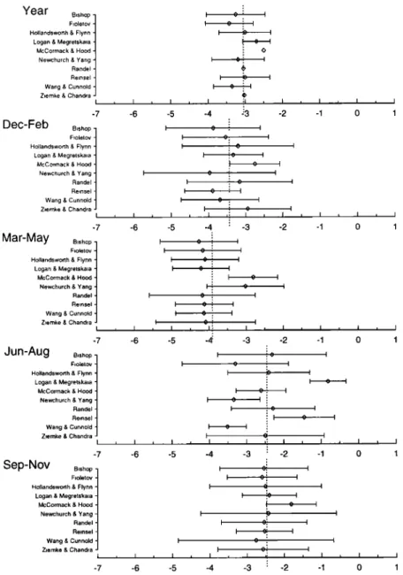
, -4 "3 I I I , I • I , l -2 -1 0 1 o , -4 o: oi o : o: o: -4" I I • I , I , I • I -7 -6 -5 -4 -3 I I -7 -6 -5 -4 -3 I i I I I I I , o: o: , I , I , I -1 0 1 • I , I , I -1 0 1 , I , I , I -1 0 1 I I , I i I , I -1 0 1 I

Figure 1. Ozone

trend

estimates

by researcher

for SAGE

I and

II 40.5 km ozone

November

1978

- April 1993,

35

o-

45øN.

Trends

are

in 10

-9 cm

'3 yr

'l. Uncertainty

intervals

are

one

standard

statistical

error.

Vertical

dotted

line is the

14,628 NEWCHURCH ET AL.: UPPER-STRATOSPHERIC OZONE TRENDS 1979-1998

through 1998. In addition, although some degree of collinearity between the solar and aerosol proxies might be expected due to their roughly similar periods, during the period of this study,

1979-1998, we calculate that the collinearity is actually insignifi- cant. This result is corroborated by the fact that the trend estimates

and uncertainties from the Dobson Umkehr measurements calcu-

lated by two independent methods, aerosol correction before ap-

plying the statistical model and aerosol correction by the statistical model, show no systematic difference.

Intercomparison of the statistical models from 10 independent groups computing trends from the Total Ozone Mapping Spec- trometer (TOMS) test data with no missing monthly values indi-

cates

agreement

between

models

to within

0.015%

yr '•, 1 standard

deviation (smaller than the average individual model trend uncer- tainty) in this most benign case (a completely continuous time se- ries). Variations in standard errors among the groups, however, were large enough to give some concern because the variations af- fect the statistical significance of the calculated trends. For exam- ple, because long-term total ozone trends near the equator border on statistical significance [WMO, 1995], the lack of proper calcu- lation of standard errors may result in nonsignificant trends' being declared statistically significant or vice versa. The results of the relatively stressing SAGE test (Figure 1) indicate agreement

within

0.1%

yr -• (1 standard

deviation)

for annual

mean

trends.

In the case of a discontinuous time series with irregular sea-

sonal

coverage,

all models

agreed

to within

0.1% yr '•, 1 standard

deviation,

for annual-mean

trends

and

to within

0.2%

yr '•, 1 stan-

dard deviation, for worst-case seasonal trends with the model-to-

model variance less than or equal to the average model-trend un- certainty. A major part of this variance could be attributed to the details of how a particular model handles missing data. Most re- searchers feel that in such situations, it is better to fit a simpler model to maintain stability, for example, by fitting seasonal trends directly or by reducing the number of harmonic terms for the sea- sonal trends and possibly also for the seasonal cycle. On the basis of these intercomparisons it seems reasonable to suggest that re- searchers provide good documentation for the features of their statistical model. Particularly, when any patterns of missing data have strong time-dependent features (e.g., missing monthly peri- ods in the SAGE data), the methods of handling the missing data

should be discussed.

This substantial agreement between the various statistical mod- els significantly enhances our confidence in their trend results and uncertainties. Variation with periods equal to or less than the QBO

exert little influence on calculated ozone trends and the aerosol ef-

fect on the Umkehr observations is well separated from the 11- year solar cycle effect resulting in decadal variations in ozone well

partitioned between volcanic and solar-cycle influences.

3. Vertical Profiles of Ozone Trends

3.1. Accounting for Aerosol Effects in Umkehr Observations

The well-known aerosol interference in the Umkehr observa-

tions is an optical interference effect on the measurements and not an in situ ozone-aerosol interaction. The following three methods

have historically been employed to identify the magnitude of and

correction for this aerosol interference: (1) theoretical radiative

transfer calculations [Mateer and DeLuisi, 1992], (2) statistical calculations (i.e., time series regression models employing exoge-

nous aerosol records) [DeLuisi et al., 1994; Reinsel et al.,1999], and (3) comparisons to other ozone measurements [Newchurch and Cunnold, 1994].

[ 1992] with aerosol data from coincident SAGE II aerosol extinc- tion measurements [Newchurch and Cunnold, 1994; Newchurch et al., 1995] along with Garmisch lidar backscatter measurements (H. J•ger, private communication, 1997) for the period prior to

1984. The lidar backscatter measurements are converted to optical depths at 320 nm by regression against SAGE-II coincident meas- urements from 1984 to 1995. The resulting continuous aerosol time series is then lagged appropriately to correct Umkehr data at various latitudes. In addition, Umkehr data during high strato- spheric aerosol optical depth periods (> 0.025 corresponding to 1 year after E1 Chichon and -•1 year after Mount Pinatubo) are omitted from the analyses. However, trends calculated with the high-aerosol periods included are not appreciably different from the trends calculated with the high-aerosol periods omitted.

Method 2 is the aerosol-correction method employed by G. Reinsel. This method uses an empirical statistical model approach in which transformed stratospheric optical thickness (transmis- sion) data serve as an exogenous explanatory variable for the Um- kehr measurements. The stratospheric aerosol optical thickness data derive from SAGE-II satellite information for the period 1985-1998. For the calculations reported here, these data were ap- pended to the optical thickness data based on composite lidar and SAGE-II measurements through December 1984 used by Reinsel et al. [ 1994]. Thus, in this statistical approach, an additional term,

¾3Z3;t, appears in the statistical model described in section 2, where Z3;t = exp[-tau(t)] -1 -• -tau(t), where tau(t) is the optical thickness.

We also note that Umkehr data were not used in the estimation for

the most extreme aerosol contamination periods (essentially,

whenever optical thickness tau(t) > 0.05, i.e., Z3;t <-0.05), roughly

November 1982 to June 1983 and November 1991 to January

1993

(for 40ø-50øN).

On the basis of the close correspondence of the results of the three historically used correction methods for the aerosol condi-

tions considered here, we conclude that the corrected Dobson

Umkehr ozone data possess less than -2% residual bias in abso-

lute ozone value due to the aerosol interference in the worst case

immediately after the 1-year omitted periods following E1 Chichon and Mount Pinatubo eruptions. The two independent Umkehr time series analyses both report trends for Umkehr stations Arosa, Boulder, and Haute Provence from 1978 to 1998 (1984-1998 at Haute Provence). These stations were chosen as a result of exten- sive examination of all Umkehr time series [I, VMO, 1998; Cunnold

et al., 2000b]. At each of these

stations,

both groups

computed

trends for total-column

ozone, for aggregate

Umkehr layers

1+2+3+4;

individual

layers

4, 5, 6, 7, and 8; and aggregate

layers

8+9+10. The two independent trend results from the northern

midlatitude

(40ø-52øN)

stations

Arosa,

Boulder,

and Haute

Pro-

vence are within 1 standard deviation in all layers. The results re- ported here are the averages of those two independent analyses.

Extensive comparisons of SAGE I/II and Dobson Umkehr

ozone profiles by Newchurch et al. [1998] indicate significant

temporal correspondence in individual layers 4 through 8. While

that study identified a significant bias between SAGE and Dobson

Umkehr increasing from 0% in layer 4 to 15% in layer 8 (SAGE

higher), the researchers found no evidence of a time dependence

in the bias for the stations analyzed in this trend paper.

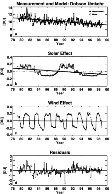
3.2. Trend Analyses of Dobson Umkehr, SAGE I/II, and SBUV(/2)

We use the Boulder Dobson Umkehr time series from 1979 to

1998 at 40-km in layer 8 (Figure 2a) to illustrate the general

analysis process. The Umkehr observations were retrieved with

To correct for the optical interference, the authors of this report the Mateer and DeLuisi [ 1992] inversion method. These monthly

employ two methods. Method 1, employed by M.J. Newchurch ozone averages, reported in Dobson Units (DU) in the layer, are

NEWCHURCH ET AL.' UPPER-STRATOSPHERIC OZONE TRENDS 1979-1998 14,629 14 12 = 10 8 6

Measurement and Model: Dobson Umkehr

ß Measurement

o

ß

0 Model

Figure 2. (a) Time series of Dobson Umkehr ozone at Boulder (solid circles) in layer 8 along with the statistical model values (open circles) and the derived trend. (b) Residuals of the statistical model fit to the monthly data. (c) Time series of the solar effect on ozone that the model calculates along with the trend in that solar effect that the model removes from the ozone trend. (d) Time se- ries of the QBO effect on ozone along with the QBO trend.

using the Mateer and DeLuisi [1992] factors in the method dis- cussed by Newchurch and Cunnold [1994]. Figure 2a displays the

measured time series of monthly values as solid circles and the full statistical-model calculations as open circles. Figure 2b dis-

plays the solar effect in Dobson Units and the calculated trend in

that solar effect that is removed from the final ozone trend. These

solar-effect trends are obviously the result of a nonsymmetric so-

lar interval that corresponds to the time interval chosen for

evaluation but are entirely accounted for by the statistical model.

The QBO effect appears in Figure 2c along with its negligible

trend. The most rigorous metric of the statistical model's adequacy

is the pattem of the residuals. These residuals appear in Figure 2d. One may see by inspection that neither trend nor temporal pattern related to the exogenous variables remains in the residual series.

The magnitude of the random fluctuations about zero is rigorously

quantified in the confidence intervals (error bars) reported below

on the various trend estimates.

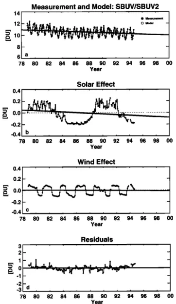
We likewise applied the Newchurch and Yang model to the

layer

8, 40ø-50øN

SAGE

I/II time

series

shown

in Figure

3 and

the

layer

8 40ø-50øN

SBUV(/2)

time

series

from

1979

to 1994

in Fig-

ure 4. The SAGE I/II observations in Figure 3 are monthly aver-

ages of version 5.96 ozone retrievals in a 5-km thick layer be-

tween 38-43 km between latitudes 40ø-50øN. Cunnold et al. [2000a] critically address the uncertainties in this data product. This data version is also extensively discussed in the WMO [1998]

assessment report. The SAGE ozone averages shown here, which include both sunrise and sunset occultation measurements, are re-

ported in the SAGE units of ozone number density versus geomet-

ric altitude. In the NIMBUS 7 SBUV version 6 and NOAA 11

(N11) SBUV/2 version 6.1.2 daily average, 50 zonal means are filtered to eliminate data taken at extreme solar-zenith angles as a

result of the N11 drifting orbit; then 100 monthly zonal means are created from these data. The monthly mean SBUV(/2) ozone data

are reported in Dobson Units within individual Umkehr layers.

Two significant consistencies emerge from the three separate

time series viewed together. First the significant ozone decrease

between the SAGE I and SAGE II time periods (1982-1984) is supported by decreases of similar magnitude (-10%) in both the Umkehr and SBUV(/2) observations. Second the amplitude of the

•6

E

Measurement and Model- SAGE 1/11

. ...

/

o.oo

.J

...

...

d

"V

il

Figure

3. As in Figure

2, except

for layer

8, 40ø-50øN,

SAGE

I/II

14,630

NEWCHURCH

ET AL.:

UPPER-STRATOSPHERIC

OZONE

TRENDS

1979-1998

Measurement and Model-SBUV/SBUV2

ß . 12 ø • 10 Year Solar Effect 0.4 ... 0.2 0.0 ... -0.2 -0.4 78 80 82 84 86 88 90 92 94 96 98 O0 Year Wind Effect 0.2

o.o •'• •

•

F• t•_.."•_t_.x._

...

.0.2fi--

•.•

• h,•

• '-•,J

• ...

3

1 ...

o .L •l•

so for the Umkehr series. The values between 1982 and 1990 in

the SBUV(/2) and Umkehr series are predominantly negative, while the 1992-1995 values are mostly positive. The SAGE II

1986-1999 values, however, are randomly distributed about zero. Therefore one could argue that an individual instrument time se- ries suggests a fit of order higher than linear, but if one takes these three series as independent realizations of the true atmosphere (as we have here), then they do not jointly justify a fit of order higher than linear. As a result, the individual linear trends are not perfect, but they are parsimonious.

To show that seasonal variation change has little effect on an- nual trend estimates in this study, we estimated seasonal ampli- tudes from TOMS test data, SBUV, and Umkehr measurements at Arosa. We use eight harmonic (12-, 6-, 4-, and 3-month sine and cosines) terms to represent the seasonal variation, instead of using only 12-month sine and cosine harmonics because, at 40 km, 6-, 4-, and/or 3-month harmonic terms are also significant. Analysis of the maximums and minimums of 2-year moving averages indi- cates small long-term changes in the seasonal amplitude in the

TOMS, SBUV, and Dobson Umkehr records. These changes of

seasonal amplitude may be real or may be caused by systematic

drifts of temperature and ozone measurements, but they do not ap- pear to be statistically significant. However, the topic is beyond

the scope of this article. While there is a possibility of the long- term change of seasonal amplitude in ozone measurements, the annual trend estimates in this study are not influenced by the sea-

sonal amplitude change, although those changes may affect sea-

sonal trend estimates. This result is not surprising because the fre-

quency associated with a linear trend is orthogonal to the fre- quency of the seasonal cycles.

A concern about the SBUV/2 data arises from the large trend

differences

between

SAGE

and SBUW2

-•1% yr

'1) reported

by

Cunnold et al. [2000a] that are much bigger than the differences in trends between SAGE and other instruments, and the known po-

tential calibration problems for SBUV/2 arising from its precess-

ing orbit. Recent evaluation of NOAA 11 SBUV/2 ozone profiles using ground-based lidars and microwaves agrees with indications from SAGE II that the NOAA 11 data contain a positive drift (i.e., values increasing relative to the correlative measurements) over

the domain 20-45 km. These SBUV/2 uncertainties are reflected in

Figure

4. As

in

Figure

2, except

for

layer

8,

40ø-50øN,

SBUV(/2)

the

following

discussions,

and

significantly

less

weight

is

given

to

ozone.

ozone

trend

estimates

from

SBUV/2

in the

final

combined

ozone

trend estimates reported in this paper.

annual variation is similar for all three sensors. The correspon-

dence

of these

three independent

ozone

time series

(with some

concern

about

the SBUV/2 data) suggests

that we should

have

considerable

confidence

in the trends

computed

from these

data

and should

expect

them

to return

similar

results.

Because

of the previous

demonstration

of the similarity

in re-

sults

of the four statistical

models

used

here, one may conclude

that

the

results

of this

particular

model

would

have

been

produced

by the

other

models

as

well.

These

measurements

are

all analyzed

and

presented

in their

native

units

to avoid

uncertainties

intro-

duced

by conversion

errors.

The magnitude

and

temporal

pattern

of the solar

effect

is essentially

the same

for all three

sensors,

as it

should

be. The temporal

evolution

of the QBO effect

is very

similar

for all three

sensors,

although

the magnitude

of the effect

on the SBUV(/2)

observations

is only

half the effect

on the Um-

kehr and SAGE measurements for unknown reasons. In all cases,

however,

the QBO effect

on the resulting

ozone

trend

is essen-

tially

zero,

as

evidenced

by the

QBO

trend

lines

in Figures

2c, 3c,

and 4c that are almost

indistinguishable

from the zero line. One

could

argue

that

the model

residuals

do not all represent

white

noise

processes

(i.e.,

are

not entirely

random).

For example,

the

residuals

prior

to 1981

lie predominantly

above

zero,

although

less

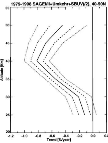
3.3. Altitude Profiles of Trends From Umkehr, SAGE I/II, and SBUV(/2)

Applying

the statistical

models

to Dobson

Umkehr,

SAGE I/II,

and SBUV(/2) time series from 1979 (November 1978 for

SBUV(/2))

to 1998

(1994

for SBUV(/2))

at 40ø-50øN

in various

layers

and combinations

of layers,

while accounting

for the poten-

tial QBO and solar effects,

produces

the ozone

annual

trends

in

Figure

5, as

percent

per

year

(% yr

'l) relative

to the

mean

of the

period.

For Umkehr

observations

we compute

trends

for layers

4-8

individually,

and

for all layers

above

seven,

8 +, plotted

as a verti-

cal bar from •-37 to 54 km. The Umkehr trends in Figure 5 are

simple averages of the two group analyses with root-mean-square

2c• error bars. Each individual-group average, however, is a vari-

ance-weighted

mean.

SAGE I/II trends

(diamonds)

are computed

layers

from 25-50 km but are not all plotted

because

those

1-km

results essentially form a smooth curve through the trends com-

puted

for 5-km thick layers

corresponding

to the Umkehr

layers.

Trends from SBUV(/2) (circles) are calculated from weekly aver-

ages

(three

daily values

required

to create

a weekly

average)

and

are reported

for layers

5-9 individually.

All error bars represent

NEWCHURCH

ET AL.' UPPER-STRATOSPHERIC

OZONE

TRENDS 1979-1998

14,631

-

,,

'• ,,

.,,,...,."'" -

_ 1979-1998 ' '"'•'

':

40-50

ø

North

,'T

-

ß SAGE

I +

SAGE

II

/

Figure

5. Ozone

trends

(% yr

'• relative

to the mean

for the pe-

riod)

at 40ø-50øN

over

the period

1979-1998

calculated

from

the

following measurement systems: Three Dobson Umkehr stations (Arosa, Boulder, and Haute Provence) reported at individual lay-

tude result primarily from uncertainties due to unresolved trend differences between sunrise and sunset observations.

For trends

calculated

from all sensors

over

the SBUV-only

time

period of 1979-1989, the general altitude structure is much the

same

as that calculated

for the longer

time period.

The layer 8 av-

erage

trend

is -0.8+0.3%

yr

4, resulting

from similar

estimates

from all three

sensors.

The other

layers

are not appreciably

differ-

ent from the longer-period trends. The confidence intervals are

generally

larger

because

of the shorter

time period.

3.4. Latitudinal Trends From SAGE and SBUV(/2)

The latitudinal coverage for the SAGE I/II observations ex-

tends

from

55øS

to 55øN.

Calculating

trends

over

the

period

1979-

1998, which comprises the entire SAGE I/II measurement set, re- sults in the altitude-latitude contour plot in Figure 6. These trends are based on concentration changes in 1-km altitude layers (the

natural coordinates for SAGE) and are referenced to the concen-

trations at the midpoint of the time series. Typical uncertainties on

the annual

trends

are 0.2-0.3%

yr

'• (95% confidence

limits).

The

altitude structure of the trends in layers 4-8 is essentially the same as reported in the WMO report over the shorter time period; how- ever, the area of significant trends is much larger in Figure 6 be-

cause of the longer time period and because of a correction for an

inadvertent error in accounting of the uncertainty resulting from

the SAGE sunrise/sunset trend differences.

In this global view the maximum ozone trends remain at 40

km (layer

8) but are larger

in the extra

tropics

(-1.0%

yr '•) than

in

the

tropics

(-0.6%

yr':).

The

minimum

trend

in layer

5 occurs

at all

latitudes with no positive trends in the tropics as were reported by WMO [1998]. In general, the SAGE I/II trends are significantly

different from zero, at the 95% confidence level (approximately

ñ0.2%

yr'•), and

at all latitudes

outside

of the tropics

for altitudes

above layer 6 (30 km). The trends exhibit remarkable hemispheric

ers 4 through 8 (triangles) and layers 8+9+10 (plotted as a vertical

bar

from

-•37

to

54

km

with

triangle);

SAGE

I/II average

sunrise

symmetry

except

in

layers

4 and

5 for

latitudes

poleward

of

40

ø.

and sunset observations (diamonds) reported at individual layers 4-10; SBUV+SBUV/2 weekly averages (circles) reported at indi- vidual layers 5 through 9. All error bars are 95% confidence inter- vals of the trend and represent statistical uncertainty only. Small vertical offsets are for clarity only (e.g., all values plotted near 30 km represent layer 6 results).

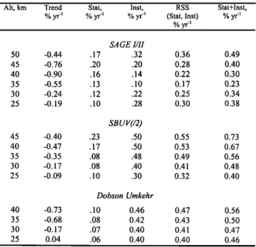
the 20 statistical-only confidence intervals. Various instrumental uncertainties are estimated in section 3.7, below.

In the upper stratosphere (i.e., layer 8), trend estimates range

from-0.5ñ0.2%yr

-• for SBUV(/2)

(circles)

to-0.9ñ0.2%

yr

': for

SAGE I/II (diamonds). The Dobson Umkehr trends for layers 8

and 8 + are both the intermediate

SAGE I/II and SBUV(/2) trends

vals overlap for the SAGE and Dobson sensors and independently for the SBUV(/2) and Dobson sensors, suggesting that the average

layer-8

trend

of approximately

-0.7ñ0.2%

yr

'l is a reasonable

es-

timate of the true atmospheric ozone decline at 40 km. A rigorous calculation is presented below.

The similarity between the independent instruments in the trends' vertical structure provides additional confidence that the true trend in atmospheric ozone is being measured. The largest de- cline occurs near layer 8, and the minimum trend is in layer 5 (---25

km), where

the trend

estimates

range

from

0.0ñ0.1%

yr '• by Dob-

son

Umkehr

to -0.2ñ0.1%

yr '• by SAGE

I/II with the SBUV(/2)

results falling between these two values. These results suggest a

layer

5 trend

of-0.1ñ0.2%

yr

'l, which

is not significantly

different

from

zero.

In layer

9, the SAGE

I/II trend

is -0.8ñ0.2%

yr

'l while

the SBUV(/2) estimate (over the shorter period through 1994) is -0.4ñ0.2 %/yr. The larger SAGE I/II error bars at 45-50 km alti-

SAGE 1/11 03 Trends 1979-1998 (%/year)

-60 -40 -20 0 20 40 60

Latitude

Figure 6. Annual ozone trends calculated from SAGE I/II obser-

vations

from 1979

to 1998

expressed

in % yr '• of the midpoint

of

the time series (1989). Results are contoured from calculations

done in 50 latitude bands and 1-km altitude intervals. Contours

differ by 0.1% yr

'• with the solid contours

indicating

zero or

negative trend. The shaded areas indicate where the trends do not

differ from zero within 95% confidence limits. The estimate of

uncertainty contains terms due to statistical uncertainty, the

SAGE-I reference height correction, and the SAGE II sun-

14,632 NEWCHURCH ET AL.: UPPER-STRATOSPHERIC OZONE TRENDS 1979-1998

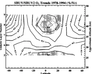
SBUV/SBUV2 0 3 Trends 1978-1994 (%/Yr)

i I ' ' ' • ' ' ' i ' ' ' i ' ' , i ' , , i 50 • 35

•

30

e•

Figure 7. Annual SBUV+SBUV/2 trend calculated •om Novem- ber 1978 through October 1994 as a hnction of latitude and Um-

kehr layer.

The •end is in % yr

'l relative

to the mean

ozone

amount •om the combined time series at each latitude and layer. The dark shading indicates the regions in which the derived •end is not si•ificantly different from zero at the 95% confidence level calculated •om statistical uncenain• only; inclusion of the in- strument e•or renders no statistically si•ificant •ends be•een

35øS

and

45•. The lighter

shading

at high

northern

and

southern

latitudes indicates regions in which the length of the time series during the winter season is compromised as a result of the NOAA 11 orbit drift (taken from WMO [ 1998, Figure 3.18].

Figure 7 shows the SBUV(/2) trends from November 1978 to

October

1994

in % yr

'l relative

to the mean

ozone

amount

from

the combined time series at each latitude and layer. The dark

shading indicates the regions in which the derived trend is not sig- nificantly different from zero at the 2• level calculated from sta-

tistical-only error bars; inclusion of the instrument error gives no

statistically

significant

trends

between

35øS

and

45øN

at the 2•

level. The lighter shading indicates regions in which the length of the time series during the winter season is compromised as a result

of the NOAA 11 orbit drift. Therefore, at these latitudes, the true annual average trend for 1978-1994 cannot be calculated. In the

Northern Hemisphere the data loss is not as extensive as in the Southern Hemisphere; therefore the northern high-latitude trends are more representative of the true annual average trends over this time period. In contrast, data loss in the Southern Hemisphere high latitudes begins as early as 1990, such that the trends plotted here are actually an average of the spring, summer, and autumn trends through 1994 and the winter trend through 1990. The largest ozone losses occur during winter in the profile data through 1990. Thus we expect an increased uncertainty in the middle- to high- latitude annual average trends in the Southern Hemisphere over this time period. Comparing the SAGE I/II trends in Figure 6 to

the SBUV(/2) trends in Figure 7 indicates similarly small trends of

0.0 to -0.3%

yr

-I in layers

5 and

6. In the upper

stratosphere,

the

altitudinal and latitudinal structures of the SAGE I/II and

SBUV(/2) trends are similar; however, the SAGE I/II trends are substantially more negative at nearly all latitudes.

The principal difference between the SAGE I/II trends from 1979 to 1998 and the SBUV(/2) trends from 1979 to 1994 should be ascribed to the SBUV/2 problems (as indicated by Cunnold et al. [2000a]). SAGE I altitudes have been adjusted as per Wang et al. [1996], and the uncertainties in those adjustments have been included in the SAGE trend error bars. Altitude registration un-

certainties between SAGE I and SAGE II in the upper stratosphere

are not large enough to contribute substantially to these differ-

ences. SAGE trends are presented on altitude surfaces whereas

SBUV trends are on pressure levels. Neither of these trend results

is affected by temperature uncertainties. However differences

between the two sets of trends might be interpreted as resulting

from long-term temperature/geopotential height trends. The larg-

est reported trends in the National Centers for Environmental Pre-

diction (NCEP) data are in the tropics in the upper stratosphere.

These amount to -•300m over the 15-year period or equivalently to

a trend

in ozone

of-•0.4%

yr

'• (based

on an ozone

scale

height

of

5 km). However, a recent reanalysis of the NCEP data as well as

an analysis of SAGE Rayleigh scattering data suggests that the

geopotential height change is significantly smaller than this. 3.5. Seasonal Trends

Investigating the layer 8 trends as a function of latitude and month, we find that the SAGE I/II (Figure 8) results show a mini-

mum

trend

of-0.7% yr

'• in the

Northern

Hemisphere

summer

and

a maximum

of-1.2% yr

'• in the winter

(i.e.,

+30%).

The Southern

Hemisphere

midlatitude

results

are-0.5 to-1.2% yr

'• (+40%).

SBUV(/2)

(Figure

9) indicates

seasonal

variation

from-0.2%

yr

'•

in Northern

Hemisphere

summer

to -0.6% yr

'• in winter.

The

Southern Hemisphere variation is somewhat larger. The magni-

tude and structure of the ozone trends' seasonal variation are

similar to the results given by WMO [1998]; however, the area of insignificance in Figure 8 is approximately half the area of the corresponding results in the WMO report. That report inadver- tently considered 1/2 the sunset/sunrise trend differences to be the 95% confidence interval limit. In this paper, as was intended in the WMO report, we consider 1/4 of the sunset/sunrise trend differ- ence to be the 95% limit [see, also, Cunnold et al., 2000a]. The

zonal seasonal variations average over the longitudinal differences

in seasonal variation. The winter-hemisphere trend maximum in the upper stratosphere is clearly evident in the SAGE I/II seasonal- trend cross sections; the equinox patterns show more symmetry between hemispheres. This seasonal pattern seen in the satellite data is consistent with results from the Dobson Umkehr analyses

at the Arosa, Boulder, and Haute Provence northern midlatitude

stations and the Perth and Lauder southern midlatitude stations.

SAGE 1/11 03 Trends Seasonal Variations (%/year)

4O -20 -40 -6O 1 3 5 7 9 11 Month

Figure

8. Seasonal

variation

of ozone

trends

in layer

8 (% yr

'l)

calculated from SAGE I/II (version 5.96, 1979-1998) for latitudes

55øS

to 55øN.

Shading

indicates

95% confidence

intervals

that

in-

clude statistical uncertainties, uncertainties due to SAGE-I altitude