Linear rank-width of distance-hereditary graphs II. Vertex-minor
obstructions
Mamadou Moustapha Kant´e1 and O-joung Kwon∗2
1Universit´e Clermont Auvergne, LIMOS, CNRS, Aubi`ere, France. 2Logic and Semantics, Technische Universit¨at Berlin, Berlin, Germany.
September 5, 2018
Abstract
In the companion paper [Linear rank-width of distance-hereditary graphs I. A polynomial-time algorithm, Algorithmica 78(1):342–377, 2017], we presented a characterization of the linear rank-width of distance-hereditary graphs, from which we derived an algorithm to compute it in polynomial time. In this paper, we investigate structural properties of distance-hereditary graphs based on this characterization.
First, we prove that for a fixed tree T , every distance-hereditary graph of sufficiently large linear rank-width contains a vertex-minor isomorphic to T . We extend this property to bigger graph classes, namely, classes of graphs whose prime induced subgraphs have bounded linear rank-width. Here, prime graphs are graphs containing no splits. We conjecture that for every tree T , every graph of sufficiently large linear rank-width contains a vertex-minor isomorphic to T . Our result implies that it is sufficient to prove this conjecture for prime graphs.
For a class Φ of graphs closed under taking vertex-minors, a graph G is called a vertex-minor obstruction for Φ if G R Φ but all of its proper vertex-minors are contained in Φ. Secondly, we provide, for each k ě 2, a set of distance-hereditary graphs that contains all distance-hereditary vertex-minor obstructions for graphs of linear rank-width at most k. Also, we give a simpler way to obtain the known vertex-minor obstructions for graphs of linear rank-width at most 1.
1
Introduction
Linear rank-width is a linear-type width parameter of graphs motivated by the rank-width of graphs [31]. The vertex-minor relation is a graph containment relation which was introduced by Bouchet [7, 8, 10, 9, 11] in his studies of circle graphs and 4-regular Eulerian digraphs. The vertex-minor relation has an important role in the theory of (linear) rank-width [27, 30, 28, 24, 29] as (linear) rank-width does not increase when taking vertex-minors of a graph. We provide concise definitions in Section 2.
The problem of computing linear rank-width has been discussed recently. Kashyap [25] proved that it is NP-hard to compute matroid path-width on binary matroids. Proposition 3.1 in [30]
∗
Supported by the European Research Council (ERC) under the European Union’s Horizon 2020 research and innovation programme (ERC consolidator grant DISTRUCT, agreement No. 648527).
0
E-mail addresses: mamadou.kante@uca.fr (M. M. Kant´e) and ojoungkwon@gmail.com (O. Kwon)
shows that the problem of determining the linear rank-width of a bipartite graph is equivalent to the problem of determining the path-width of a binary matroid, and from this relation, we can show that computing linear rank-width is NP-hard in general. Adler and the authors of this paper [3] proved that the linear rank-width of distance-hereditary graphs, which are graphs of rank-width 1, can be computed in time Opn2log nq where n is the number of vertices in an input graph. Jeong, Kim, and Oum [23] showed that, there is a constructive algorithm to test whether a given graph has linear rank-width at most k in time f pkq ¨ n3 for some function f . Using this, they also proved that for every fixed integer w, there is a polynomial-time algorithm to compute linear rank-width on graphs of rank-width w.
In this paper, we focus on structural aspects of linear rank-width. The first result of the Graph Minor series papers is that for a fixed tree T , every graph of sufficiently large path-width contains a minor isomorphic to T [32], and this was later used by Blumensath and Courcelle [6] to define a hierarchy of incidence graphs based on monadic second-order transductions. In order to obtain a similar hierarchy for graphs, still based on monadic second-order transductions, Courcelle [14] asked whether for a fixed tree T , every bipartite graph of sufficiently large linear rank-width contains a vertex-minor isomorphic to T . We conjecture that it is true for any graph.
Conjecture 1.1. For every fixed tree T , there is an integer f pT q such that every graph of linear rank-width at least f pT q contains a vertex-minor isomorphic to T .
We show that Conjecture 1.1 is true if and only if it is true in prime graphs with respect to split decompositions [16]. A split in a graph is a vertex partition pA, Bq such that |A|, |B| ě 2 and the set of edges joining A and B induces a complete bipartite subgraph. Prime graphs are graphs without splits and they form, with complete graphs and stars, the basic graphs in the theory of canonical split decompositions developed by Cunningham [16]. They are also considered when studying the rank-width of graphs because the rank-width of a graph is the maximum rank-width over all its prime induced subgraphs.
We prove the following.
Theorem 1.2. Let p be a positive integer and let T be a tree. Let G be a graph such that every prime induced subgraph of G has linear rank-width at most p. If G has linear rank-width at least 40pp ` 2q|V pT q|, then G contains a vertex-minor isomorphic to T .
A graph G is distance-hereditary if for every connected induced subgraph H of G and two vertices v and w in H, the distance between v and w in H is the same as their distance in G. It is known that every prime induced subgraph of a distance-hereditary graph has size at most 3 [10]. Together with this fact, our result implies that Conjecture 1.1 is also true for distance-hereditary graphs.
To prove Theorem 1.2, we essentially prove that for a fixed tree T , every graph admitting a canonical split decomposition whose decomposition tree has sufficiently large path-width contains a vertex-minor isomorphic to T . Combined with a relation between the linear rank-width of a graph and the path-width of its canonical split decomposition, we obtain Theorem 1.2. We will obtain such a relation in Section 4. The vertex-minor relation cannot be replaced with the induced subgraph relation because there is a cograph admitting a canonical split decomposition whose decomposition tree has sufficiently large path-width [13, 21], but cographs have no P4 as an induced subgraph.
In the second part, we investigate the set of distance-hereditary vertex-minor obstructions for graphs of bounded linear rank-width. A graph is a vertex-minor obstruction for graphs of linear
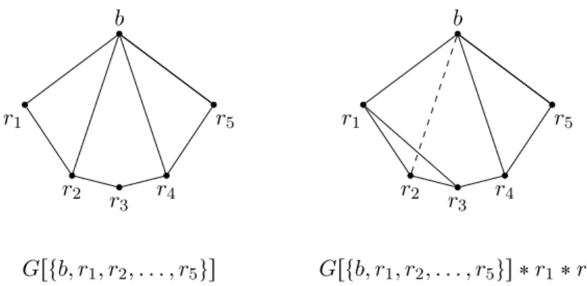
Figure 1: The three vertex-minor obstructions for graphs of linear rank-width at most 1. The first two graphs are distance-hereditary.
rank-width k if it has linear rank-width k ` 1 and every proper vertex-minor has linear rank-width k. Robertson and Seymour [33] showed that for every infinite sequence G1, G2, . . . of graphs, there exist Gi and Gj with i ă j such that Gi is isomorphic to a minor of Gj. In other words, graphs are well-quasi-ordered under the minor relation. Interestingly, this property implies that for any proper class C of graphs closed under taking minors, the set of minor obstructions for C is finite.
Oum [27, 29] obtained an analogous result for the vertex-minor relation; for every infinite sequence G1, G2, . . . of graphs of bounded rank-width, there exist Gi and Gj with i ă j such that Gi is isomorphic to a vertex-minor of Gj. We can obtain the following as a corollary.
Theorem 1.3 (Oum [27]). For every class C of graphs with bounded rank-width that is closed under taking vertex-minors, there is a finite list of graphs G1, G2, . . . , Gm such that a graph is in C if and only if it has no vertex-minor isomorphic to Gi for some i P t1, 2, . . . , mu.
Theorem 1.3 implies that for every integer k, the class of all graphs of (linear) rank-width at most k can be characterized by a finite list of vertex-minor obstructions. However, it does not give any explicit number of necessary vertex-minor obstructions or bound on the size of such graphs. Oum [30] proved that for each k, the size of a vertex-minor obstruction for graphs of rank-width at most k is at most p6k`1´ 1q{5. For linear rank-width, obtaining such an upper bound on the size of vertex-minor obstructions remains an open problem. Jeong, Kwon, and Oum [24] showed that the number of vertex-minor obstructions for linear rank-width at most k is at least 2Ωp3kq.
Adler, Farley, and Proskurowski [1] obtained the set of all three vertex-minor obstructions for graphs of linear rank-width at most 1, depicted in Figure 1, two of which are distance-hereditary. In this paper, we construct a set of graphs containing all vertex-minor obstructions for graphs of linear rank-width at most k that are distance-hereditary. This is an analogous result to the characterization of acyclic minor obstructions for graphs of path-width at most k, investigated by Takahashi, Ueno, and Kajitani [34], and Ellis, Sudborough, and Turner [19]. As a similar work, Koutsonas, Thilikos, and Yamazaki [26] characterized matroid obstructions for bounded matroid path-width that are cycle matroids of outerplanar graphs.
Lastly, we obtain simpler proofs of known characterizations of graphs of linear rank-width at most 1 [1, 12].
The paper is organized as follows. Section 2 provides some preliminary concepts, including linear rank-width and vertex-minors. In Section 3, we introduce necessary notions regarding split decom-positions, and restate the structural characterization of linear rank-width on distance-hereditary graphs. Section 4 presents a relation between the linear rank-width of a graph whose prime induced subgraphs have bounded linear rank-width and the path-width of its decomposition tree. From this, we prove Theorem 1.2 in Section 5. In Section 6, we provide a way to generate all vertex-minor obstructions for graphs of bounded linear rank-width that are distance-hereditary graphs. Section 7 presents simpler proofs for known characterizations of the graphs of linear rank-width at most 1.
2
Preliminaries
In this paper, graphs are finite, simple and undirected. Our graph terminology is standard, see for instance [18]. Let G be a graph. We denote the vertex set of G by V pGq and the edge set by EpGq. For X Ď V pGq, we denote by GrXs the subgraph of G induced by X, and let G´X :“ GrV pGqzXs. For v P V pGq, we write G ´ x for G ´ txu. For F Ď EpGq, let G ´ F :“ pV pGq, EpGqzF q. For a vertex x of G, let NGpxq be the set of neighbors of x in G and we call |NGpxq| the degree of x in G. Two vertices x and y are twins if NGpxqztyu “ NGpyqztxu. An edge e of a connected G is a cut-edge if G ´ e is disconnected. A vertex v in a connected graph G is a cut vertex if G ´ v is disconnected. A connected graph is 2-connected if it has at least 3 vertices and has no cut vertices. A tree is a connected graph containing no cycles. A vertex of degree one in a tree is called a leaf. A subcubic tree is a tree with maximum degree at most three, and a path is a tree with maximum degree at most two. The length of a path is the number of its edges. A star is a tree with a distinguished vertex, called its center, adjacent to all other vertices. A complete graph is a graph with all possible edges. A graph G is called distance-hereditary if for every pair of two vertices x and y of G the distance of x and y in G equals the distance of x and y in any connected induced subgraph containing both x and y [4]. It is well-known that a graph is distance-hereditary if and only if it can be obtained from a single vertex by repeated addition of degree one vertices and twins [22]. An induced cycle of length at least 5 is not distance-hereditary.
A subset F of the edge set of G is called a matching if no two edges in F share an end vertex. For an edge e of a graph G, we denote by G{e the graph obtained by contracting e. A graph H is a minor of a graph G if H is obtained from a subgraph of G by contractions of edges. 2.1 Linear rank-width
For sets R and C, an pR, Cq-matrix is a matrix whose rows and columns are indexed by R and C, respectively. For an pR, Cq-matrix M and subsets X Ď R and Y Ď C, let M rX, Y s be the submatrix of M whose rows and columns are indexed by X and Y , respectively.
Let G be a graph. We denote by AG the adjacency matrix of G over the binary field; that is, for v, w P V pGq, AGrv, ws “ 1 if v is adjacent to w, and AGrv, ws “ 0, otherwise. For a graph G, let cutrk˚
G : 2V pGqˆ 2V pGq Ñ Z be a function such that cutrk˚GpX, Y q :“ rankpAGrX, Y sq for all X, Y Ď V pGq, where rank is computed over the binary field. The cut-rank function of G is the function cutrkG: 2V pGq Ñ Z where for each X Ď V pGq,
cutrkGpXq :“ cutrk˚GpX, V pGqzXq.
An ordering px1, . . . , xnq of the vertex set V pGq is called a linear layout of G. If |V pGq| ě 2, then the width of a linear layout px1, . . . , xnq of G is defined as
max
1ďiďn´1tcutrkGptx1, . . . , xiuqu,
and if |V pGq| “ 1, then the width is defined to be 0. The linear rank-width of G, denoted by lrwpGq, is defined as the minimum width over all linear layouts of G.
Caterpillars and complete graphs have linear rank-width at most 1. Ganian [20] gave a char-acterization of graphs of linear rank-width at most 1, and called them thread graphs. Adler and Kant´e [2] showed that linear rank-width and path-width coincide on forests, and therefore, there is
v w G w v G ^ vw Figure 2: An example of pivoting.
a linear-time algorithm to compute the linear rank-width of forests. It is easy to see that the linear rank-width of a graph is the maximum over the linear rank-widths of its connected components.
For a linear layout L of a graph G and v, w P V pGq, we denote v ďL w if v “ w or v appears before w in the linear layout. For two orderings pv1, v2, . . . , vnq and pw1, w2, . . . , wmq, we denote
pv1, v2, . . . , vnq ‘ pw1, w2, . . . , wmq :“ pv1, v2, . . . , vn, w1, w2, . . . , wmq.
2.2 Vertex-minors
For a graph G and a vertex x of G, the local complementation at x in G is an operation to replace the subgraph induced by the set of neighbors of x with its complement. The resulting graph is denoted by G ˚ x. If a graph H can be obtained from G by applying a sequence of local complementations, then G and H are called locally equivalent. A graph H is called a vertex-minor of a graph G if H can be obtained from G by applying a sequence of local complementations and deletions of vertices. Bouchet [11] observed that local complementation does not change the cut-rank function. This directly implies that every vertex-minor H of G satisfies that lrwpHq ď lrwpGq.
Lemma 2.1 (Bouchet [11]; See Corollary 2). Let G be a graph and let x be a vertex of G. Then for every subset X of V pGq, we have cutrkGpXq “ cutrkG˚xpXq.
For an edge xy of G, let W1 :“ NGpxq X NGpyq, W2 :“ pNGpxqzNGpyqqztyu, and W3 :“ pNGpyqzNGpxqqztxu. The pivoting on xy of G, denoted by G ^ xy, is the operation to flip the adjacencies between distinct sets Wi and Wj, and swap the vertices x and y. Flipping the adjacency between two vertices v and w is an operation that add an edge if there was no edge between v and w, and remove an edge, otherwise. It is known that G ^ xy “ G ˚ x ˚ y ˚ x “ G ˚ y ˚ x ˚ y [30, Proposition 2.1]. See Figure 2 for an example.
2.3 Path-width
A path decomposition of a graph G is a pair pP, Bq, where P is a path and B “ pBtqtPV pP q is a family of vertex subsets of G such that
1. for every v P V pGq there exists t P V pP q such that v P Bt, 2. for every uv P EpGq there exists t P V pP q such that tu, vu Ď Bt, 3. for every v P V pGq, the set tt P V pP q : v P Btu induces a subpath of P .
The width of a path decomposition pP, Bq is defined as maxt|Bt| : t P V pP qu ´ 1. The path-width of G, denoted by pwpGq, is defined as the minimum width over all path-decompositions of G.
It is well known that if H is a minor of G, then pwpHq ď pwpGq. Robertson and Seymour [32] first proved that for a fixed tree T , every graph of sufficiently large path-width contains a minor isomorphic to T . The necessary function was optimized by Bienstock, Robertson, Seymour, and Thomas [5].
Theorem 2.2 (Bienstock, Robertson, Seymour, and Thomas [5]). For every forest F , every graph with path-width at least |V pF q| ´ 1 has a minor isomorphic to F .
We recall the following theorem which characterizes the path-width of trees and is used for computing their path-width in linear time.
Theorem 2.3 (Ellis, Sudborough, and Turner [19]; Takahashi, Ueno, and Kajitani [34]). Let T be a tree and let k be a positive integer. The following are equivalent.
(1) T has path-width at most k.
(2) For every node x of T , at most two of the subtrees of T ´ x have path-width k and all other subtrees of T ´ x have path-width at most k ´ 1.
(3) T has a path P such that for each node v of P and each connected component T1 of T ´ v not containing a node of P , pwpT1q ď k ´ 1.
3
Linear rank-width of distance-hereditary graphs
In this section, we recall the characterization of the linear rank-width of distance-hereditary graphs investigated by Adler and the authors of this paper [3]. For this characterization, we need to introduce split decompositions and the new notion of limbs introduced in the previous paper. We will follow the definition for split decompositions used by Bouchet [10].
A split in a connected graph G is a vertex partition pX, Y q of G such that |X|, |Y | ě 2 and cutrkGpXq “ 1. Prime graphs are connected graphs that do not have a split. Note that every connected graph with at most 3 vertices is a prime graph, by definition. Also, one can observe that every connected graph on 4 vertices admits a split, and it is not a prime graph.
A marked graph is a connected graph D with a matching M pDq where every edge in M pDq is a cut-edge. Every edge in M pDq is called a marked edge, and the end vertices of marked edges are called marked vertices. The connected components of D ´ M pDq are called bags of D. The edges in EpDqzM pDq are called unmarked edges, and the vertices that are not marked are called unmarked vertices.
If pX, Y q is a split in a marked graph G, then we construct a new marked graph D such that • V pDq “ V pGq Y tx1, y1
u for two distinct new vertices x1, y1
R V pGq, • EpDq “ EpGrXsq Y EpGrY sq Y tx1y1u Y E1 where
E1 :“ tx1x : x P X and there exists y P Y such that xy P EpGquY ty1y : y P Y and there exists x P X such that xy P EpGqu, • x1y1 is a marked edge, and all edges in E1 are unmarked edges.
B
B
Figure 3: An example of replacing a bag B with its simple decomposition. Circles indicate bags and dotted edges indicate marked edges.
The marked graph D is called a simple decomposition of G. See Figure 3 for an example.
A split decomposition of a connected graph G is a marked graph D defined inductively to be either G or a marked graph defined from a split decomposition D1 of G by replacing a bag with its simple decomposition. For a marked edge xy of a marked graph D, the recomposition of D along xy is the marked graph pD ^ xyq ´ tx, yu. For a split decomposition D, let GrDs denote the graph obtained from D by recomposing all marked edges. Note that if D is a split decomposition of G, then GrDs “ G.
Since each marked edge of a split decomposition D is a cut-edge and all marked edges form a matching, if we contract all unmarked edges in D, then we obtain a tree. We call it the decomposition tree of G associated with D and denote it by TD. To distinguish the vertices of TD from the vertices of G or D, the vertices of TD will be called nodes. For a node v of TD, we write bagDpvq to denote the bag of D with which it is in correspondence, and for a bag B of D, we write nodeDpBq to denote the node of TD with which it is in correspondence. Two bags of D are called adjacent bags if their corresponding nodes in TD are adjacent. A sequence of bags B1´ B2´ ¨ ¨ ¨ ´ Bm is called a path of bags if for each i P t1, 2, . . . , m ´ 1u, Bi and Bi`1 are adjacent bags, and all of B1, B2, . . . , Bm are pairwise distinct. Clearly, for two bags B and B1, there is a unique path of bags from B to B1, which corresponds to the path from nodeDpBq to nodeDpB1q in TD. We denote by distDpB, B1q the distance from nodeDpBq to nodeDpB1q in TD; in other words, it is one less than the number of bags in the unique path of bags from B to B1 in D.
3.1 Canonical split decompositions and local complementations
A split decomposition is called canonical if each bag is either a prime graph, a star, or a complete graph, and every recomposition of a marked edge in D results in a split decomposition without the same property. The following is due to Cunningham and Edmonds [15], and Dahlhaus [17]. Theorem 3.1 (Cunningham and Edmonds [15]; Dahlhaus [17]). Every connected graph G has a unique canonical split decomposition, up to isomorphism, and it can be computed in time Op|V pGq|` |EpGq|q.
A bag is called a prime bag if it is a prime graph on at least 5 vertices, and a bag is called a complete bag or a star bag if it is a complete graph or a star, respectively.
Let D be a split decomposition of a connected graph G with bags that are either a prime graph, a complete graph or a star. The type of a bag of D is either P , K, or S depending on whether it is a prime graph, a complete graph, or a star, respectively. The type of a marked edge uv is AB where A and B are the types of the bags containing u and v respectively. If A “ S or B “ S, then we can replace S by Sp or Sc depending on whether the end of the marked edge is a leaf or the center of the star, respectively. Bouchet characterized when it becomes a canonical split decomposition. Theorem 3.2 (Bouchet [10]). Let D be a split decomposition of a connected graph whose bags are either a prime graph, a complete graph, or a star. Then D is a canonical split decomposition if and only if it has no marked edge of type KK or SpSc.
We will use the following characterizations of trees and of distance-hereditary graphs. Theorem 3.3 (Bouchet [10]).
(1) A connected graph is distance-hereditary if and only if every bag of its canonical split decom-position is of type K or S.
(2) A connected graph is a tree if and only if every bag of its canonical split decomposition is a star bag whose center is an unmarked vertex.
We now relate the split decompositions of a graph and the ones of its locally equivalent graphs. Let D be a split decomposition of a connected graph. A vertex v of D represents an unmarked vertex x (or is a representative of x) if either v “ x or there is a path of even length from v to x in D starting with a marked edge such that marked edges and unmarked edges appear alternately in the path. Two unmarked vertices x and y are linked in D if there is a path from x to y in D such that unmarked edges and marked edges appear alternately in the path. Linkedness of unmarked vertices exactly represents the adjacency relation between those vertices in the original graph. Lemma 3.4 (Adler, Kant´e, and Kwon [3]). Let D be a split decomposition of a connected graph G. Let v1 and w1 be two vertices in a same bag of D, and let v and w be two unmarked vertices of D represented by v1 and w1, respectively. The following are equivalent.
1. v and w are linked in D. 2. vw P EpGq.
3. v1w1 P EpDq.
A local complementation at an unmarked vertex x in a split decomposition D, denoted by D ˚ x, is the operation to replace each bag B containing a representative w of x with B ˚ w. Bouchet observed that D ˚ x is a split decomposition of GrDs ˚ x, and M pDq “ M pD ˚ xq. Two split decompositions D and D1 are locally equivalent if D can be obtained from D1 by applying a sequence of local complementations at unmarked vertices. As expected, this local complementation also preserves the property that the split decomposition is canonical.
Lemma 3.5 (Bouchet [10]). Let D be the canonical split decomposition of a connected graph G. If x is a vertex of G, then D ˚ x is the canonical split decomposition of G ˚ x.
D v z v D ∗ v v z D ^ vz
Figure 4: Examples of local complementation and pivoting in a split decomposition.
Let x and y be linked unmarked vertices in a split decomposition D, and let P be the path in D linking x and y such that unmarked edges and marked edges appear alternately in the path. Note that if B is a bag of type S containing an unmarked edge of P , then the center of B is a representative of either x or y. The pivoting on xy of D, denoted by D ^ xy, is the split decomposition obtained as follows: for each bag B containing an unmarked edge of P , if v, w P V pBq represent respectively x and y in D, then we replace B with B ^ vw. It is worth noticing that by Lemma 3.4, we have vw P EpBq, hence B ^ vw is well-defined.
Lemma 3.6 (Adler, Kant´e, and Kwon [3]). Let D be a split decomposition of a connected graph G. If xy P EpGq, then D ^ xy “ D ˚ x ˚ y ˚ x.
3.2 Removing vertices
Let G be a distance-hereditary graph and let D be its split decomposition. Let S be a vertex set of G. We explain how we transform D into a split decomposition of G ´ S. Note that the split decomposition obtained from D by removing vertices in S is not necessarily a split decomposition because the resulting marked graph may have bags of size at most 2. In this case, we need to recompose a marked edge incident with each bag of size at most 2 unless the resulting marked graph has at most two vertices.
Suppose D is canonical. We frequently consider connected components T of D ´V pBq, for a bag B of D. This will be used to define limbs in the next subsection. For a bag B of D and a connected component T of D ´ V pBq, let us denote by ζbpD, B, T q and ζcpD, B, T q the end vertices of the marked edge in D linking B and T that are in V pBq and in V pT q respectively. Subscripts b and c stand for bag and component, respectively. We always treat T as a canonical split decomposition and regard ζcpD, B, T q as an unmarked vertex.
3.3 Limbs and characterization of linear rank-width
To present the characterization of the linear rank-width of distance-hereditary graphs, we need the new notion called limbs [3]. For an unmarked vertex y in D and a bag B of D containing a marked vertex representing y, let T be the connected component of D ´ V pBq containing y, and let v :“ ζcpD, B, T q and w :“ ζbpD, B, T q. We define the limb L :“ LDrB, ys with respect to B and y as follows:
B
y
B
y
Figure 5: An example of a limb LDrB, ys.
2. if B is of type S and w is a leaf, then L :“ T ´ v,
3. if B is of type S and w is the center, then L :“ T ^ vy ´ v.
While T is a canonical split decomposition, L may not be a canonical split decomposition, because deleting v may create a bag of size 2. We analyze the cases when such a bag appears, and describe how to transform it into a canonical split decomposition. Suppose that a bag B1 of size 2 appears in L. If B1 has no adjacent bags in L, then B1 itself is a canonical split decomposition. We may assume there is a bag adjacent to B1.
1. (B1 has one adjacent bag B 1.)
If v1 P V pB1q is the marked vertex adjacent to a vertex of B1 and r is the unmarked vertex of B1 in L, then we remove the bag B1 and replace v
1 with r. In other words, we recompose along the marked edge connecting B1 and B
1. 2. (B1 has two adjacent bags B
1 and B2.)
If v1 P V pB1q and v2 P V pB2q are the two marked vertices that are adjacent to the two marked vertices of B1, then we remove B1 and add a marked edge v
1v2. If the new marked edge v1v2 is of type KK or SpSc, then by recomposing along v1v2, we finally transform the limb into a canonical split decomposition.
Let LCDrB, ys be the canonical split decomposition obtained from LDrB, ys and we call it the canonical limb. Let LGDrB, ys be the graph obtained from LDrB, ys by recomposing all marked edges. For a bag B of D and a connected component T of D ´ V pBq, we define fDpB, T q as the linear rank-width of LGDrB, ys for some unmarked vertex y P V pT q. It was shown that fDpB, T q does not depend on the choice of y.
Proposition 3.7 (Adler, Kant´e, and Kwon; Proposition 3.4 of [3]). Let B be a bag of D and let y be an unmarked vertex of D represented by a vertex w in B. Let x P V pGrDsq. If an unmarked vertex y1 is represented by w in D ˚ x, then LG
DrB, ys is locally equivalent to LGD˚xrpD ˚ xqrV pBqs, y1s. Therefore, fDpB, T q “ fD˚xppD ˚ xqrV pBqs, Txq where T and Tx are the components of DzV pBq and pD ˚ xqzV pBq containing y, respectively.
As a variant of Theorem 2.3, distance-hereditary graphs of bounded linear rank-width can be characterized using limbs.
Theorem 3.8 (Adler, Kant´e, and Kwon [3]). Let k be a positive integer and let D be the canonical split decomposition of a connected distance-hereditary graph G. Then the following are equivalent. (1) G has linear rank-width at most k.
(2) For each bag B of D, D ´ V pBq has at most two connected components T such that fDpB, T q “ k, and every other connected component T1 of D ´ V pBq satisfies that f
DpB, T1q ď k ´ 1. (3) TD has a path P such that for each node v of P and each connected component H of D ´
V pbagDpvqq containing no bags bagDpwq with w P V pP q, fDpbagDpvq, Hq ď k ´ 1.
4
Path-width of decomposition trees
To prove Theorem 1.2, we derive a relation between the linear rank-width of a graph whose prime induced subgraphs have bounded linear rank-width and the path-width of its decomposition tree. Proposition 4.1. Let p be a positive integer. Let G be a connected graph whose prime induced subgraphs have linear rank-width at most p, and let D be the canonical split decomposition of G, and let TD be the decomposition tree of G associated with D. Then lrwpGq ď 2pp ` 2qppwpTDq ` 1q. We prove Proposition 4.1 by induction on the path-width of TD. If its path-width is 0, then it consists of one node, and the result directly follows from the given condition that every prime induced subgraph has linear rank-width at most p. Note that complete graphs and stars have linear rank-width at most 1. We assume that the path-width of TD is at least 1. Using Lemma 2.3, T contains a path P such that for each node v of P and each connected component T1 of T ´ v not containing a node of P , pwpT1
q ď k ´ 1. So, by induction, we can obtain an upper bound of the linear rank-width of split decompositions corresponding to such components T1. From this, we will obtain an upper bound of the linear rank-width of the whole graph.
We need the following lemma. We point out that Lemma 4.2 does not require D to be a canonical split decomposition, and this relaxation will be useful for an easier argument in the main proof.
Lemma 4.2. Let k and p be positive integers. Let B be a bag of a split decomposition D with two unmarked vertices a and b such that for every connected component H of D ´V pBq, lrwpGrHsq ď k. If B has a linear layout of width at most p whose first and last vertices are a and b respectively, then GrDs has a linear layout of width at most 2p ` k whose first and last vertices are a and b respectively.
Proof. Let G :“ GrDs, and let LB :“ pw1, w2, . . . , wmq be a linear layout of B of width at most p such that a “ w1 and b “ wm. For each j P t1, 2, . . . , mu,
1. if wj is an unmarked vertex, then let Lj :“ pwjq, and
2. if wj “ ζbpD, B, Hq for some connected component H of D ´ V pBq, then let Lj be a linear layout of GrHs ´ ζcpD, B, Hq having width at most k.
We define L :“ L1‘ L2 ‘ ¨ ¨ ¨ ‘ Lm. We observe that L is a linear layout of G. For each j P t1, 2, . . . , mu, we choose an unmarked vertex yj represented by wj. If wj is an unmarked vertex, then yj “ wj.
We claim that L has width at most 2p`k. It is sufficient to prove that for every w P V pGqzta, bu, cutrkGptv : v ďL wuq ď 2p ` k. Let w P V pGqzta, bu and let Sw :“ tv : v ďL wu and Tw :“ V pGqzSw.
Let Hj be a connected component of D ´ V pBq such that ζbpD, B, Hjq “ wj. Observe that if all vertices in V pHjq X V pGq are contained in Sw, then all vertices in V pHjq X V pGq that have a neighbor in Tw have exactly the same set of neighbors in Tw, which is NGpyjq X Tw. Therefore, when we compute the rank of the matrix ApGqrSw, Tws, we can replace all vertices in V pHjq X V pGq with yj. The same observation holds for connected components fully contained in Tw. Also, for two distinct connected components Hj1, Hj2 of D ´ V pBq where all vertices of V pHj1q X V pGq are
contained in Sw and all vertices of V pHj2q X V pGq are contained in Tw, y1 and y2 are adjacent in G
if and only if ζbpD, B, H1q is adjacent to ζbpD, B, H2q in B. This is an implication of Lemma 3.4. Having it, we can observe that if w is an unmarked vertex in B, then
cutrkGpSwq “ cutrkBptv : v ďLB wuq ď p.
Thus, we may assume that w is contained in some connected component H of D ´ V pBq. Let j P t1, 2, . . . , mu such that ζbpD, B, Hq “ wj.
Note that H is the unique component of D ´ V pBq possibly intersecting both Sw and Tw. Since all vertices of V pHq X V pGq having a neighbor in V pGqzV pHq have the same neighborhood in V pGqzV pHq (that is, pV pHq X V pGq, V pGqzV pHqq is a split), we have
(1) cutrk˚GpSw, TwzV pHqq ď maxtcutrkBptv : v ďLB wj´1uq, cutrkBptv : v ďLB wjuqu ď p.
(2) cutrk˚
GpSwzV pHq, Twq ď maxtcutrkBptv : v ďLB wj´1uq, cutrkBptv : v ďLB wjuqu ď p.
(3) cutrk˚GpSwX V pHq, TwX V pHqq ď k. Therefore, we have
cutrkGpSwq ď cutrk˚GpSw, TwzV pHqq ` cutrk˚GpSwzV pHq, Twq ` cutrk˚GpSwX V pHq, TwX V pHqq
ď p ` p ` k ď 2p ` k.
We conclude that L is a linear layout of G of width at most 2p ` k whose first and last vertices are a and b, respectively.
Proof of Proposition 4.1. We prove it by induction on k :“ pwpTDq. If k “ 0, then TD consists of one node, and G is either a prime graph, a complete graph, or a star. Note that complete graphs and stars have linear rank-width at most 1. Thus, we have lrwpGq ď p ď 2pp ` 2q. We may assume that k ě 1.
Since pwpTDq “ k ě 1, by Theorem 2.3, there exists a path P :“ v1v2¨ ¨ ¨ vnin TD such that for each node v in P and each connected component T of TD´ v not intersecting P , pwpT q ď k ´ 1. For each i P t1, 2, . . . , nu, let Bi :“ bagDpviq. By induction hypothesis, for each i P t1, 2, . . . , nu and each connected component H of D ´ V pBiq not intersecting
Ť
1ďjďnV pBjq, we have lrwpGrHsq ď 2pp ` 2qk.
Now, let us modify the given canonical split decomposition by two additional unmarked vertices so that we can easily apply Lemma 4.2. For each i P t1, 2, . . . , nu, let LBi be a linear layout of Bi
D
1D
2D
3D
4a1 b1 a2 b2 a3 b3 a4 b4
Figure 6: The sequence of sub-decompositions D1, . . . , Dn in Proposition 4.1.
is unmarked. Similarly, we add a twin of the last vertex of LBn in Bn such that the added vertex is
unmarked. Let a1 be the vertex added to B1 and bn be the vertex added to Bn. It is not difficult to see that B1 has a linear layout of width at most p whose first vertex is a1, and Bn has a linear layout of width at most p whose last vertex is bn.
Assume for a moment that n ě 2. For each i P t1, 2, . . . , n ´ 1u, let bi and ai`1 be the marked vertices of Bi and Bi`1, respectively, such that biai`1 is the marked edge connecting Bi and Bi`1. If bi is not the end vertex of LBi, then we reorder LBi so that bi is the end vertex. Similarly, if ai`1
is not the first vertex of LBi`1, then we reorder LBi`1 so that ai`1 is the first vertex. Until now,
the width of each LBi may increase by at most 2. This is because the rank of a matrix increase
by at most 1 when we move one element in the column indices (resp. the row indices) to the row indices (resp. the column indices).
Note that the resulting decomposition is not necessarily canonical, as we may add a twin of a vertex in a prime graph. But this is not a problem when we apply Lemma 4.2. By the above modification, we know that for each i P t1, 2, . . . , nu, there is a linear layout of Bi of width at most p ` 2 whose first and last vertices are ai and bi, respectively.
We define the following sub-decompositions. See Figure 6 for an illustration. If n “ 1, then let D1:“ D. Otherwise,
1. let D1 be the connected component of D ´ V pB2q containing B1,
2. let Dn be the connected component of D ´ V pBn´1q containing Bn, and
3. for each i P t2, 3, . . . , n ´ 1u, let Di be the connected component of D ´ pV pBi´1q Y V pBi`1qq containing Bi.
We regard the vertices ai and bi as unmarked vertices of Di.
Recall that pwpT q ď k ´1 for every node v of P and every connected component T of TD´ v not intersecting P . Therefore, lrwpGrHsq ď 2pp ` 2qk, for each connected component H of Di´ V pBiq, by induction hypothesis. Thus, by Lemma 4.2, GrDis has a linear layout Li of width at most 2pp ` 2q ` 2pp ` 2qk “ 2pp ` 2qpk ` 1q whose first and last vertices are ai and bi, respectively. For each i P t1, 2, . . . , nu, let L1
i be the linear layout obtained from Li by removing ai and bi. Then it is not hard to check that
L11‘ L12‘ ¨ ¨ ¨ ‘ L1n
is a linear layout of G having width at most 2pp ` 2qpk ` 1q. We conclude that lrwpGq ď 2pp ` 2qppwpTDq ` 1q.
For distance-hereditary graphs, the following establishes a lower bound and the tight upper bound of linear rank-width with respect to the path-width of their canonical split decompositions.
Proposition 4.3. Let D be the canonical split decomposition of a connected distance-hereditary graph G. Then 12pwpTDq ď lrwpGq ď pwpTDq ` 1.
The upper bound part is tight. For instance, every complete graph with at least two vertices has linear rank-width 1 and the path-width of its decomposition tree has path-width 0. Also, for each odd integer k “ 2n ` 1 with n ě 1, every complete binary tree of height k (each path from a leaf to the root has distance k) has linear rank-width rk{2s “ n ` 1, and its decomposition tree has path-width rpk ´ 1q{2s “ n. (Note that the linear rank-width and the path-width of a tree are the same [2].) We will need the following lemmas.
Lemma 4.4. Let G be a graph and let uv P EpGq. Then pwpGq ď pwpG{uvq ` 1.
Proof. Let pP, Bq be an optimal path-decomposition of G{uv, and let z be the contracted vertex in G{uv. It is not hard to check that a new path-decomposition obtained by removing z and adding u and v in each bag containing z is a path-decomposition of G. We conclude that pwpGq ď pwpG{uvq ` 1.
Lemma 4.5. Let G be a graph. Let u be a vertex of degree 2 in G such that v1, v2 are the neighbors of u in G and v1v2 R EpGq. Then pwpGq ď pwpG{uv1{uv2q ` 1.
Proof. Let w be the contracted vertex in G{uv1{uv2, and let pP, Bq be an optimal path-decomposition of G{uv1{uv2 of width t :“ pwpG{uv1{uv2q. We may assume that no two adjacent bags in pP, Bq are equal.
We obtain a path-decomposition pP, B1
q from pP, Bq by replacing w with v1 and v2 in all bags containing w. Since no two adjacent bags in pP, Bq are equal, no two adjacent bags in pP, B1q are equal.
We first assume that there are two adjacent bags B1 and B2 in pP, B1q containing both v1 and v2, respectively. We obtain a path-decomposition pP1, B2q from pP, B1q by subdividing the edge between B1 and B2, and adding a new bag B1 “ pB1X B2q Y tuu. Since B1 and B2 are not the same, |B1X B2| ď t ` 1 and therefore, |B1| ď t ` 2. Thus, pP1, B2q is a path-decomposition of G of width at most t ` 1, and pwpGq ď pwpG{uv1{uv2q ` 1.
Now we may assume that there is only one bag B in pP, B1
q containing both v1 and v2. In this case, since v1v2 R EpGq, we can obtain a path decomposition of G by replacing this bag B with a sequence of two bags B1 and B2, where B1 :“ Bztv2u Y tuu and B2 :“ Bztv1u Y tuu. This implies that pwpGq ď pwpG{uv1{uv2q ` 1.
We are now ready to prove Proposition 4.3. We need the split decomposition characterization of graphs of linear rank-width at most 1 proved by Bui-Xuan, Kant´e, and Limouzy [12] for the base case, which can be easily obtained by Theorem 3.8. We give a proof of this characterization in Theorem 7.1.
Proof of Proposition 4.3. (1) Let us first prove that pwpTDq ď 2 lrwpGq by induction on the linear rank-width of G. Let k :“ lrwpGq. If k “ 0, then G consists of a vertex, and pwpTDq “ 0. If k “ 1, then by Theorem 7.1, TD is a path and we have pwpTDq ď 1 ď 2k. Thus, we may assume that k ě 2. By Theorem 3.8, there exists a path P in TD such that
• for every node v in P and every connected component H of D ´ V pbagDpvqq containing no bag in tbagDpwq | w P V pP qu, fDpbagDpvq, Hq ď k ´ 1.
Let v be a node of P and C be a connected component of D ´ V pbagDpvqq containing no bag bagDpwq with w P V pP q. Let y be an unmarked vertex of C represented by ζcpD, bagDpvq, Cq, and let L :“ LCDrV pbagDpvqq, ys. By induction hypothesis, the decomposition tree TL of L has path-width at most 2k ´ 2. We claim that pwpTCq ď 2k ´ 1, where TC is the decomposition tree of C. By the definition of canonical limbs, either TL“ TC or TL is obtained from TC using one of the following operations:
1. Removing a node of degree 1.
2. Removing a node of degree 2 with its neighbors v1, v2 and adding an edge v1v2. 3. Removing a node of degree 2 with its neighbors v1, v2 and identifying v1 and v2.
The first two cases can be regarded as contracting one edge. So, pwpTCq ď pwpTLq ` 1 ď p2k ´ 2q ` 1 “ 2k ´ 1 by Lemma 4.4. The last case corresponds to contracting two edges incident with a vertex of degree 2. By Lemma 4.5, pwpTCq ď pwpTLq ` 1 ď 2k ´ 1.
Therefore, for each node v of P and each connected component T1 of T
D´ v not containing a node of P we have that pwpT1
q ď 2k ´ 1. By Theorem 2.3, TD has path-width at most 2k, as required.
(2) We prove that lrwpGq ď pwpTDq ` 1 by induction on the path-width of TD. Let k :“ pwpTDq If k “ 0, then TD consists of one node. Since G is distance-hereditary, G should be a star or a complete graph, and therefore, we have lrwpGq ď 1 “ pwpTDq ` 1. We may assume that k ě 1.
By Theorem 2.3, there exists a path P “ v0v1¨ ¨ ¨ vnvn`1 in TD such that for every node v in P and every connected component F of TD´ v containing no nodes of P , pwpF q ď k ´ 1. Let v be a node of P and let C be a connected component of D ´ V pbagDpvqq conaining no bags bagDpwq with w P V pP q. By induction hypothesis, GrCs has linear rank-width at most pk ´ 1q ` 1 “ k. By the definition of limbs, we conclude that fDpbagDpvq, Cq ď k. Thus, by Theorem 3.8, we conclude that lrwpGq ď k ` 1.
We could not confirm that the lower bound in Proposition 4.3 is tight. We leave the following as an open question.
Question 1. Let D be the canonical split decomposition of a connected distance-hereditary graph G. Is it true that pwpTDq ď lrwpGq?
5
Containing a tree as a vertex-minor
In this section, we prove our first main result.
Theorem 1.2. Let p be a positive integer and let T be a tree. Let G be a graph such that every prime induced subgraph of G has linear rank-width at most p. If lrwpGq ě 40pp ` 2q|V pT q|, then G contains a vertex-minor isomorphic to T .
To prove it, we observe that the decomposition tree of the canonical split decomposition of G has large path-width using Theorem 4.1. The main argument of this section is that if G admits a canonical split decomposition whose decomposition tree has sufficiently large path-width, then G contains a vertex-minor isomorphic to T .
v v1 v2 v3 v4 v5 v6 v v1 v2 v3 v4 v5 v6 p2 p1
Figure 7: Splitting an edge in Lemma 5.1.
We first prove that every tree is a vertex-minor of some subcubic tree having slightly more vertices. For a tree T , we denote by φpT q the sum of the degrees of vertices of T whose degrees are at least 4. Every subcubic tree T satisfies that φpT q “ 0.
Lemma 5.1. Let k be a positive integer and let T be a tree with φpT q “ k. Then T is a vertex-minor of a tree T1 with φpT1
q “ k ´ 1 and |V pT1q| “ |V pT q| ` 2.
Proof. Since φpT q ě 1, T has a vertex of degree at least 4. Let v P V pT q be a vertex of degree at least 4, and let v1, v2, . . . , vm be its neighbors. We obtain T1 from T by replacing the edge vv1 with the path vp2p1v1, removing vv2 and adding an edge between p1 and v2. It is easy to verify that pT1^ p1p2q ´ tp1, p2u “ T . We depict this procedure in Figure 7. We observe that p1 and p2 are vertices of degree at most 3 in T1, and the degree of v in T1 is one less than the degree of v in T . Therefore, we have φpT1q “ k ´ 1.
Lemma 5.2. Every tree T is a vertex-minor of a subcubic tree T1 with |V pT1
q| ď 5|V pT q|. Proof. By Lemma 5.1, T is a vertex-minor of a subcubic tree T1 with |V pT1
q| ď |V pT q| ` 2φpT q. Since φpT q ď 2|EpT q| ď 2|V pT q|, we conclude that |V pT1q| ď |V pT q| ` 2φpT q ď 5|V pT q|.
We recall that by (2) of Theorem 3.3, a connected graph is a tree if and only if every bag of its canonical split decomposition is a star bag whose center is an unmarked vertex. The basic strategy is to extract the canonical split decomposition of a subcubic tree from the canonical split decomposition of G. To do this, we will obtain a star from each prime bag, without changing too much the shape of the obtained canonical split decomposition. Lemma 5.4 describes how to obtain a star from a prime graph as a vertex-minor, without applying local complementations at some special vertices, which will correspond to marked vertices.
We observe that every prime graph on at least 5 vertices is 2-connected. This is because if a connected graph G contains a cut vertex v and T1, T2, . . . , Tm are connected components of G ´ v, then ´ V pT1q Y tvu, Ť jPt2,...,muV pTjq ¯
is a split of G. We use this observation in Lemma 5.4. Lemma 5.3. Let abc be an induced path in a 2-connected graph G. By applying local complemen-tations at vertices in V pGqzta, bu, we can obtain G1 locally equivalent to G such that G1
rta, b, cus is a triangle.
Proof. As b is not a cut vertex of G, there is a path from a to c in G ´ b. Let r1r2¨ ¨ ¨ rs be the shortest path from c “ r1 to a “ rsin G ´ b. Note that s ě 3 as a is not adjacent to c. See Figure 8 for an illustration.
We prove by induction on s that Grtb, r1, r2, . . . , rsus can be transformed into an induced path acb by applying local complementations only at vertices in tr1, r2, . . . , rs´1u. We illustrate this
b r1 r2 r 3 r4 r5 Grtb, r1, r2, . . . , r5us b r1 r2 r 3 r4 r5 Grtb, r1, r2, . . . , r5us ˚ r1˚ r2 Figure 8: Reducing from Grtb, r1, r2, . . . , rsus in Lemma 5.3.
procedure in Figure 8. Assume s “ 3. If b is adjacent to r2, then we remove this edge by applying a local complementation at c “ r1. And then we apply a local complementation at r2 to create an edge between a and c. Then abc becomes a triangle.
We assume s ě 4. Similarly, if b is adjacent to r2, then we remove this edge by applying a local complementation at c “ r1, and then we apply a local complementation at r2 to create an edge between c and r3. If b is not adjacent to r2, then we apply a local complementation at r2 to create an edge between c and r3. Let G1 be the resulting graph. Then r1r3r4¨ ¨ ¨ rs is an induced path in G1 ´ b. Thus, by induction hypothesis, we can obtain G2 locally equivalent to G1rtb, r1, r3, r4, . . . , rsus by applying local complementations only at vertices in tr1, r3, . . . , rs´1u such that G2rta, b, cus is a triangle.
Lemma 5.4. Let G be a prime graph on at least 5 vertices, and let a, b, c P V pGq. Then there exists a sequence x1, x2, . . . , xtof vertices in V pGqzta, bu (not necessarily all distinct) such that acb is an induced path of G ˚ x1˚ x2˚ ¨ ¨ ¨ ˚ xt.
Proof. We first create a triangle or an induced path of length 2 on ta, b, cu by applying local complementations at vertices in V pGqzta, b, cu. For this argument, a, b, c are symmetric. Without loss of generality, we assume the distance between a and b is at most the distance between a and c or between b and c. Let P “ p1p2¨ ¨ ¨ pm be a shortest path from a “ p1 to b “ pm in G. By the distance property, c R V pP q. We define
G1:“ #
G ˚ p2˚ p3˚ ¨ ¨ ¨ ˚ pm´1 if m ě 3,
G otherwise.
It is not difficult to observe that a and b are adjacent in G1. Now, we take a shortest path Q “ q1q2¨ ¨ ¨ qn from c “ q1 to qnP ta, bu in G1. We define
G2 :“ #
G1˚ q2˚ q3˚ ¨ ¨ ¨ ˚ qn´1 if n ě 3,
G1 otherwise.
We observe that c has a neighbor on ta, bu in G2. Furthermore, if a and b are not adjacent in G2, it means that the last local complementation removed this edge, and it implies that c should be adjacent to both a and b in G2. Therefore, either G2rta, b, cus is a triangle or an induced path of length 2.
T
RT
1 v w zB
F
RF
1 v w zP
Figure 9: An example application of Lemma 5.5.
We do not want to apply local complementation at a, b to create a required induced path. If acb is already an induced path, then we are done. If G2rta, b, cus is a triangle, then we apply local complementation at c. Therefore, we may assume that abc or bac is an induced path. Note that G2 is 2-connected.
Case 1. abc is an induced path in G2.
We apply Lemma 5.3. Then by applying local complementations at vertices in V pGqzta, bu, we can obtain G3 locally equivalent to G2 such that G3rta, b, cus is a triangle. By applying a local complementation at c, we obtain the required path.
Case 2. bac is an induced path in G2.
We apply Lemma 5.3. Then by applying local complementations at vertices in V pGqzta, bu, we can obtain G3 locally equivalent to G2 such that G3rta, b, cus is a triangle. By applying a local complementation at c, we obtain the required path.
We conclude the lemma.
Starting from a split decomposition whose decomposition tree is a subdivision of a huge binary tree, we will extract a split decomposition of some fixed binary tree. To do this, we need to explain how we sequentially transform each bag into a star whose center is unmarked. Lemma 5.5 deal with the case when a bag has two neighbor bags, and Lemma 5.6 deal with the case when a bag has three neighbor bags.
A canonical split decomposition D is rooted if we distinguish a leaf bag and call it the root of D. Let D be a rooted canonical split decomposition with root bag R. A bag B is a descendant of a bag B1 if B1 is on the path of bags from R to B in D. If B is a descendant of B1 and B and B1 are adjacent bags, then we call B a child of B1 and B1 the parent of B. A bag in D is called a non-root bag if it is not the root bag.
Lemma 5.5. Let D be a rooted canonical split decomposition of a connected graph with root bag R and let B be a non-root bag of D such that
• the parent of B is a star and ζcpD, B, TRq is a leaf.
Then by possibly applying local complementations at unmarked vertices of D contained in V pT1q Y V pBq and deleting some unmarked vertices in B, we can transform D into a canonical split decom-position D1 containing a bag P such that
1. D1´ V pP q consists of exactly two connected components F
R and F1, 2. FR“ TR or FR“ TR˚ ζcpD, B, TRq,
3. F1 is locally equivalent to T1, and
4. P is a star bag whose center is unmarked.
Proof. Let v :“ ζbpD, B, TRq and w :“ ζbpD, B, T1q. Let y be an unmarked vertex in D represented by w. See Figure 9 for the setting.
First assume that B is a star bag. Since ζcpD, B, TRq is a leaf, v is not the center of B. If its center is unmarked, then we are done. We may assume the center of B is w. Since |V pBq| ě 3, B contains at least one unmarked vertex, which is adjacent to w. We choose an unmarked leaf vertex z in B. We observe that y is linked to z, that is, yz P EpGq. Then in D ^ yz, z becomes the center of a star, and TR does not change. Also, T1 is changed to the decomposition obtained from T1 by pivoting yz1 where z1 “ ζ
cpD, B, T1q. Thus, the resulting decomposition satisfies the required property. If B is a complete bag, then we choose an unmarked vertex in B, and apply a local complementation at this vertex. Then the resulting decomposition satisfies the required property.
Now, suppose B is a prime bag. Choose an unmarked vertex z of B that is adjacent to w. Since a prime graph with at least 5 vertices is 2-connected, there is always an unmarked vertex adjacent to w. Note that y and z are linked.
Let B1be the child of B. If B1is a star bag whose center is adjacent to B, then by pivoting yz we transform B1 into a star bag having ζcpD, B, T1q as a leaf. If B1 is a complete bag, then we apply a local complementation at y. In the resulting decomposition, either B1 is a prime bag or ζcpD, B, T1q is a leaf of a star bag. Let B1 be the bag modified from B in the resulting decomposition. Note that B1 is still a prime graph by Lemma 2.1.
We apply Lemma 5.4 with pa, b, cq “ pv, w, zq. By Lemma 5.4, we can modify B1into an induced path vzw by only applying local complementations at unmarked vertices in B1 and removing all unmarked vertices in B1 except z. Note that the marked edges incident with B1 are still marked edges that cannot be recomposed, as both have types SpSp or SpP . Let D1 be the modified decomposition and let P be the new bag in D1 modified from B1. Then D1 ´ V pP q has two connected components FR and F1 where
• FR“ TR or FR“ TR˚ ζcpD, B, TRq, • F1 is locally equivalent to T1, and • P is a star whose center is unmarked, as required.
Lemma 5.6. Let D be a rooted canonical split decomposition of a connected graph with root bag R and let B be a non-root bag of D such that
• D ´ V pBq has exactly three connected components T1, T2, and TR where TR contains R, • the distance from nodeDpBq to nodeDpRq is at least 3 in TD,
• the parent P1 of B and its parent P2 satisfy that nodeDpP1q and nodeDpP2q have degree 2 in TD,
• P1 and P2 are stars whose centers are unmarked, and
• for each i P t1, 2u, the child Bi of B in Ti satisfies that nodeDpBiq has degree 2 in TD. Then by possibly applying local complementations at unmarked vertices of D contained in V pT1q Y V pT2q Y V pBq Y V pP1q Y V pP2q and deleting some unmarked vertices in V pT1q Y V pT2q Y V pBq Y V pP1q Y V pP2q and recomposing some marked edges, we can transform D into a canonical split decomposition D1 containing a bag P such that
1. D1´ V pP q consists of exactly three connected components F
1, F2, and FR, 2. FR“ TR´ pV pP1q Y V pP2qq,
3. for each i P t1, 2u, Fi is locally equivalent to Ti or Ti´ V pBiq, and 4. P is a star bag whose center is unmarked.
Proof. For each i P t1, 2u, let xibe the center of Pi, and let v :“ ζbpD, B, TRq, and for each i P t1, 2u, let vi:“ ζbpD, B, Tiq, and yi be an unmarked vertex represented by vi.
We first deal with an easier case.
Case 1. B is either a star or a complete graph, and has an unmarked vertex.
The case when B is a complete graph is depicted in Figure 10. We first transform B into a star whose center is unmarked. Let z be an unmarked vertex in B.
Assume B is a star. Since ζcpD, B, TRq is a leaf of a star, v is not the center of B. We may assume that the center of B is either v1 or v2. By symmetry, we may assume it is v1. In this case, y1 and z are linked in D. Thus, B becomes a star whose center is z in D ^ y1z. If B is a complete bag, then we apply a local complementation at z. Then B becomes a star whose center is z. Note that in any case, TR does not change by this local complementation as ζcpD, B, TRq is a leaf of a star, and Ti becomes a split decomposition locally equivalent to Ti.
Let D1 be the resulting decomposition. Lastly, we transform D1 into a split decomposition D2 as follows:
1. We pivot x1x2 and then remove all unmarked vertices contained in P1 and P2.
2. We recompose marked edges incident with P1 and P2. Equivalently, we remove all vertices in P1 and P2 in the decomposition, and add a new marked edge between v and the marked vertex in the parent of P2 that is adjacent to P2.
Note that D2 is canonical, as the new marked edge has the same type as before. Thus, we obtained a required decomposition.
Now, we may assume that either B is a prime bag, or |V pBq| “ 3. Case 2. |V pBq| “ 3.
B x2 x1 z (a) D B x2 x1 z (b) D ˚ z B x2 x1 z (c) D ˚ z ^ x1x2 Bz (d) D ˚z ^x1x2´tx1, x2u
B x2 x1 y1 y2 (a) D B x2 x1 y1 y2 (b) D ˚ y1 B x2 y1 y2 (c) D ˚ y1^ x1x2´ x1 B y1 y2 x2 (d) Pivot x2y1
An example case is depicted in Figure 11.
Since |V pBq| “ 3, B is either a star or a complete graph. We first modify B into a star whose center is v1. First assume that B is a star. Since ζcpD, B, TRq is a leaf of a star, the center of B is either v1 or v2. We may assume the center of B is v2. Since v1 is adjacent to v2, y1 and y2 are linked in D. Then B becomes a star whose center is v1 in D ^ y1y2. If B is a complete bag, then we apply local complementation at y1. Then B becomes a star whose center is v1. Note that TR does not change by this local complementation as ζcpD, B, TRq is a leaf of a star and the center of the parent of B is unmarked. Let D1 be the resulting decomposition.
Let w be the marked vertex in P2 that is adjacent to P1. We transform D1 into a split decom-position D2 as follows:
1. We pivot x1x2.
2. We delete the vertices of V pP1q, and add a marked edge between v and w. 3. We recompose the new marked edge vw (it is of type SpSc).
Observe that the bag B1 in D
2 obtained by merging B and P2 is a star whose center is v1, and it contains an unmarked vertex x2. Moreover, D2 is canonical. Lastly, we pivot y1x2. Then B1 becomes a star whose center is x
2. Note that the connected components of D2 ´ V pB1q are respectively TR ´ pV pP1q Y V pP2qq and F1 and F2 such that Fi is locally equivalent to Ti for i P t1, 2u.
Now, it remains to show when B is a prime bag. We reduce this case to Case 1 or Case 2 applying Lemma 5.4. Note that in the previous cases, we deduce that Fi is locally equivalent to Ti for each i P t1, 2u. But when we transform B into a star bag, we may merge B with one of its child bags.
Case 3. B is a prime bag.
Note that applying a local complementation at an unmarked vertex in B does not change the fact that y1is represented by v1. This is because the alternating path from y1 to v1does not change when we apply a local complementation at an unmarked vertex in B.
We apply Lemma 5.4 with pa, b, cq “ pv, v2, v1q so that B is transformed into an indued path vv1v2. Note that applying a local complementation at v1 can be simulated by applying a local complementation at y1. Since B is a prime graph on at least 5 vertices, by Lemma 5.4, we can modify B into an induced path vv1v2by only applying local complementations at unmarked vertices in B and y1. Then we remove all the other vertices of B.
Note that the marked edge connecting B and P1 is still a valid marked edge as ζcpD, B, TRq is a leaf of a star. However, for i P t1, 2u, the marked edge incident with vi and ζcpD, B, Tiq may have type SpSc. In this case, we recompose this marked edge so that the resulting decomposition is canonical.
Let D1 be the modified decomposition. Since both nodeDpP1q and nodeDpP2q have degree 2 in TD, the bag B1 of D1 modified from B still has 3 adjacent bags in D1. As B1 is star bag of D1, we can reduce the remaining steps to Case 1 or Case 2 depending on the size of B1, from which we can construct the required canonical split decomposition.
We are ready to prove the main result of the section. We note that for a graph H, any subdivision of H contains a vertex-minor isomorphic to H. We will use this fact. For a tree T , let ηpT q be the tree obtained from T by replacing each edge with a path of length 4.
Proof of Theorem 1.2. Let t :“ |V pT q| and suppose that lrwpGq ě 40pp ` 2qt. By Lemma 5.2, there exists a subcubic tree T1 such that T is a vertex-minor of T1and |V pT1q| ď 5t. We consider the tree ηpT1
q which is the tree obtained from T1 by replacing each edge with a path of length 4. Observe that |V pηpT1
qq| ď 20t.
Let D be the canonical split decomposition of G and let TD be the decomposition tree of D. Since lrwpGq ě 40pp ` 2qt, by Proposition 4.1, pwpTDq ě 20t ´ 1. Since |V pηpT1qq| ď 20t, from Theorem 2.2, TD contains a minor isomorphic to ηpT1q. Since the maximum degree of ηpT1q is at most 3, T
D contains a subgraph T1 that is isomorphic to a subdivision of ηpT1q. Let D1:“ Dr
Ť
vPV pT1qV pbagDpvqqs. Observe that D1 is not necessarily a decomposition of an induced subgraph of G, as the unmarked vertex which was a marked vertex before does not correspond to a real vertex of G. To make it as a decomposition of an induced subgraph of G, we obtain a new decomposition D2 from D1 as follows:
• For every unmarked vertex x of D1 that was a marked vertex in D, there is a vertex y P V pGq represented by x in D. We choose such a vertex and replace x with y.
We can observe that D2 is a canonical split decomposition of an induced subgraph of G, and TD2
is isomorphic to TD1.
We choose a leaf bag R2of D2and regard it as the root of D2. We first transform R2into a star where the marked vertex in R2 is a leaf by applying local complementations at unmarked vertices of D2.
(˚) Let v be the marked vertex of R2, and v1 be a neighbor of v in R2, and w be an unmarked vertex of D2 represented by v. If R2 is a star whose center is unmarked, then we do nothing. If R2 is a star whose center is v, then we pivot v1w. If R2 is a complete bag, then we apply local complementation at v1. Then R
2 becomes a star whose center is unmarked.
Assume R2 is a prime bag and let C be the child of R2. If C is a star whose center c is adjacent to v, then we do a pivot at v1w to turn C into a star with c as a leaf. If C is a complete graph, then we apply a local complementation at w. The bag modified from C is either a prime graph or a star whose leaf is adjacent to v. Let R1
2 be the resulting bag from R2.
Now, we choose one more unmarked vertex v2 in R1
2 adjacent to v. Such a vertex exists as R1
2 is 2-connected. Applying Lemma 5.4 to R12 with pa, b, cq “ pv, v1, v2q, there exists a sequence x1, x2, . . . , x` of vertices in V pR21qztv, v1u such that vv2v1 is an induced path of R1
2˚ x1˚ x2˚ ¨ ¨ ¨ ˚ x`. We apply this sequence of local complementations and then remove all vertices in R1
2 except v, v1, and v2. By the previous procedure, the resulting decomposition is canonical and the bag modified from R1
2 is a star whose center is unmarked.
Let D3 be the resulting decomposition, and R3 be the root bag that is modified from R2. Note that TD3 is isomorphic to TD2.
As TD3 is isomorphic to a subdivision of ηpT
1
q, there is a subdivision mapping g from T1 to TD3
such that for each edge e of T1, gpeq is a path of length at least 4. Note that gpV pT1
qq is exactly the set of all leaves and all vertices of degree at least 3 in TD3.
A bag B is processed if every bag on the path from B to the root bag is a star whose center is unmarked. Let B1, B2, . . . , Bm be an ordering of bags in tbagD3pvq : v P gpV pT
1
qqu such that • for each i P t2, 3, . . . , mu, every ascendant bag of Bi in the set tbagD3pvq : v P gpV pT
1qqu is contained in tB1, B2, . . . , Bi´1u.
Such an ordering can be found using a BFS. For each i P t2, 3, . . . , mu, let F pBiq be the bag B in tB1, B2, . . . , Bi´1u such that B is an ascendant bag of Bi, and B is closest to Bi. We will define below a sequence F1, F2, . . . , Fm of rooted canonical split decompositions such that nodeD3pBjq P V pTFiq for 1 ď i, j ď m, and for convenience we keep continuing calling Bj the bag
bagFipnodeD3pBjqq.
For j P t1, 2, . . . , mu, let F1, F2, . . . , Fj be a maximal sequence of rooted canonical split decom-positions such that
• D3 “ F1,
• for each i P t1, 2, . . . , j ´ 1u, GrFi`1s is a vertex-minor of GrFis, • in Fi with i P t1, 2, . . . , ju,
– B1, B2, . . . , Bi are processed,
– for ` P t2, 3, . . . , iu, distFipB`, F pB`qq ě 1,
– if B P tBi`1, Bi`2, . . . , Bmu is a bag where F pBq is processed, then distFipB, F pBqq ě 3,
– if B P tBi`1, Bi`2, . . . , Bmu is a bag where F pBq is not processed, then distFipB, F pBqq ě
4.
– nodeD3pR3q P V pTFiq and Fi is rooted at bagFipnodeD3pR3qq
By (˚), B1 “ R3 is processed. Thus, F1 is indeed a sequence satisfying those conditions when j “ 1. We claim that j “ m. In other words, all bags in tbagD3pvq : v P gpV pT1qqu can be sequentially processed.
Claim 1. j “ m.
Proof. Suppose for contradiction that j ă m. We may assume that Bj`1is not processed in Fj, otherwise, F1, F2, . . . , Fj, Fj`1 is a longer sequence satisfying the required conditions. Clearly, F pBj`1q is processed. The induction hypothesis for j implies that distFjpBj`1, F pBj`1qq ě 3.
Let F pBj`1q “ U1´ U2´ ¨ ¨ ¨ ´ Uy “ Bj`1 be the path of bags in Fj from F pBj`1q to Bj`1. We recursively apply Lemma 5.5 to U2, U3, . . . , Uy´1 so that the bag modified from each of U2, U3, . . . , Uy´1 is a star whose center is unmarked. Note that when we apply Lemma 5.5 to U2, U3, . . . , Uy´1, the decomposition tree does not change.
After then, we apply Lemma 5.6 to Bj`1 so that the bag modified from Bj`1 is a star whose center is unmarked. When we apply Lemma 5.6 to Bj`1, some child bags of Bj`1may be merged with Bj`1. Thus if U is a bag with F pU q “ Bj`1, then the value distFjpU, Bj`1q may decrease
by at most 1.
Let Fj`1 be the resulting decomposition. We can verify that in Fj`1, • B1, B2, . . . , Bj, Bj`1 are processed,
• for ` P t2, 3, . . . , j ` 1u, distFj`1pB`, F pB`qq ě 1,
• if B P tBj`2, Bj`3, . . . , Bmu is a bag where F pBq is processed, then distFj`1pB, F pBqq ě 3,
• if B P tBj`2, Bj`3, . . . , Bmu is a bag where F pBq is not processed, then distFj`1pB, F pBqq ě
• nodeD3pR3q P V pTFiq and Fi is rooted at bagFipnodeD3pR3qq
This contradicts the maximality of the sequence. We conclude that j “ m. ♦ Let D4 :“ Fm. Note that TD4 is isomorphic to a subdivision of T
1, and every bag of D
4 is a star whose center is unmarked. Therefore, GrD4s is isomorphic to a tree that can be obtained from a subdivision of T1 by adding some leaves, and in particular, GrD
4s contains an induced subgraph isomorphic to a subdivision of T1. Thus, G contains a vertex-minor isomorphic to T1, and also contains a vertex-minor isomorphic to T , as required.
6
Distance-hereditary vertex-minor obstructions for graphs of bounded
linear rank-width
In this section, we describe a way to generate all vertex-minor obstructions for graphs of bounded linear rank-width that are distance-hereditary graphs. It generalizes the constructions developed by Jeong, Kwon, and Oum [24].
For a distance-hereditary graph G, a connected distance-hereditary graph G1 is a one-vertex DH-extension of G if G “ G1´ v for some vertex v P V pG1q. For convenience, if G1 is a one-vertex DH-extension of G, and D and D1 are canonical split decompositions of G and G1 respectively, then D1 is also called a one-vertex DH-extension of D.
Let D1, D2 and D3 be three canonical split decompositions. For each i P t1, 2, 3u, let D1i be a one-vertex DH extension of Di with a new unmarked vertex wi and such that wi is not contained in a star bag centered at wi. Furthermore, we choose an unmarked vertex zi linked to wi. Let B be a complete graph or a star, on three vertices v1, v2, v3. For each i P t1, 2, 3u, let Di2 be a split decomposition such that
1. if B is a complete graph, then D2
i :“ Di1˚ wi, 2. if B is a star with center vi, then Di2:“ D1i^ wizi, 3. if B is a star with vi a leaf, then D2i :“ Di1.
We let N pD1, D2, D3, Kq be the set of all possible canonical split decompositions obtained from the disjoint union of such D2
1, D22, D23 and a complete bag B on three vertices v1, v2, v3, by adding the marked edges v1w1, v2w2, and v3w3. For i P t1, 2, 3u, we let N pD1, D2, D3, pS, iqq be the set of all possible canonical split decompositions obtained from the disjoint union of such D2
1, D22, D32 and a star bag B on three vertices v1, v2, v3 whose center is vi, by adding the marked edges v1w1, v2w2, and v3w3.
For a set D of canonical split decompositions, we let
∆pDq :“ tN pD1, D2, D3, Kq | D1, D2, D3 P Du
Y tN pD1, D2, D3, pS, iqq | D1, D2, D3 P D, i P t1, 2, 3uu, D`:“ D Y tD1: D1 is a one vertex DH-extension of D P Du.
For each non-negative integer k, we recursively construct the set Ψk of canonical split decom-positions as follows.
B1 B2 1) B1 B2 2) B1 B2 3) B1 B2 4)
Figure 12: A shorten procedure described in Lemma 6.2.
1. Ψ0:“ tK2u (K2 is the canonical split decomposition of itself.) 2. For k ě 0, let Ψk`1:“ ∆pΨ`kq.
We prove the following.
Theorem 6.1. Let k be a non-negative integer. Every distance-hereditary graph of linear rank-width at least k ` 1 contains a vertex-minor isomorphic to a graph whose canonical split decomposition is isomorphic to a decomposition in Ψk.
We prove some intermediate lemma.
Lemma 6.2. Let D be the canonical split decomposition of a connected distance-hereditary graph containing two distinct bags B1 and B2, and for each i P t1, 2u, let Ti be the connected component of D ´ V pBiq such that Ti contains B3´i. If
• ζbpD, B1, T1q is not the center of a star and • B2 is a star bag and ζbpD, B2, T2q is a leaf of B2, then there exists a canonical split decomposition D1 such that
1. GrDs has GrD1
s as a vertex-minor, 2. DrV pT2qzV pT1qs “ D1rV pT2qzV pT1qs, 3. DrV pT1qzV pT2qs “ D1rV pT1qzV pT2qs, and
4. either B1 and B2 are adjacent in D1, or there is a path of bags B1´ B ´ B2 in D1 such that |V pBq| “ 3 and B is a star bag whose center is unmarked.