Computing the minimum distance between a point and a NURBS curve

HAL Id: inria-00518359

https://hal.inria.fr/inria-00518359

Submitted on 17 Sep 2010

HAL is a multi-disciplinary open access

archive for the deposit and dissemination of

sci-entific research documents, whether they are

pub-lished or not. The documents may come from

teaching and research institutions in France or

abroad, or from public or private research centers.

L’archive ouverte pluridisciplinaire HAL, est

destinée au dépôt et à la diffusion de documents

scientifiques de niveau recherche, publiés ou non,

émanant des établissements d’enseignement et de

recherche français ou étrangers, des laboratoires

publics ou privés.

Computing the minimum distance between a point and

a NURBS curve

Xiao-Diao Chen, Jun-Hai Yong, Guozhao Wang, Jean-Claude Paul, Gang Xu

To cite this version:

Xiao-Diao Chen, Jun-Hai Yong, Guozhao Wang, Jean-Claude Paul, Gang Xu. Computing the

min-imum distance between a point and a NURBS curve. Computer-Aided Design, Elsevier, 2008, 40

(10-11), pp.1051-1054. �10.1016/j.cad.2008.06.008�. �inria-00518359�

1052 X.-D. Chen et al. / Computer-Aided Design 40 (2008) 1051–1054

Fig. 1. Four cases of f(u)in a sub-interval. f(u)will reach the local minimum only in the case of1(d).

method of [5] is time-consuming, and propose a method based on the control polygon of the NURBS curve [2]. Their method is efficient for planar NURBS curve, but it may fail for the NURBS curve in R3space [20]. Selimovic presents a hyperplane clipping method for the point projection of NURBS curves [19]. If all the control points of the NURBS curve and the test point are on the different sides of a hyperplane which passes through an end-point of the curve and perpendicular to the direction from the test point to the end-point, then the end-point is the nearest point. In these methods, when the sub-curve is flat enough or the parameter interval of the sub-curve is smaller than a given tolerance, the subdivision of the sub-curves is terminated and numerical methods such as Newton’s method are utilized to solve the local solution. The subdivision theory of NURBS curves can be found in [21–23].

For B-spline surfaces, Chen et al. present a method based on the subdivision of a B-spline function instead of the subdivision of the B-spline surface. They provide a sufficient condition that the nearest point is on the boundary curves of a B-spline surface, and show that the new exclusion criteria in that paper are superior to other comparable exclusion criteria. However, they do not cover the rational case, i.e., neither NURBS curves or NURBS surfaces.

This paper presents a circular clipping method for the point projection problem of NURBS curves. Based on the objective squared distance function between the test point and the curve, we provide a sufficient condition whether a curve is outside a circle (or a sphere in R3space). The elimination circle is utilized, whose center point is just the test point p. We also provide a method to obtain the initial value of the radius of the elimination circle. We eliminate the curve parts which are outside the elimination circle. Then, we iteratively subdivide the remaining curve parts to obtain a new but smaller radius of the elimination circle, and do the similar elimination work for these remaining curve parts. A simple termination condition is provided. We show that the new termination condition will be satisfied after a finite number of subdivision steps, even when the remaining parameter interval is large or the sub-curve is not flat enough. This termination condition leads to little subdivision time in the new method. When the subdivision process is terminated, the objective squared distance function is convex and has exactly one minimum in its local parameter domain, which ensures that the Newton method will converge an accurate result [13,24]. Examples are shown to illustrate the efficiency and robustness of the new method.

This paper is organized as follows. Section2presents the outline of the new algorithm. Section3compares the new method with other comparable methods. Analyses and examples are also shown in this section. Some conclusions are drawn at the end of this paper.

2. Outline of the circular clipping algorithm

This section presents a circular clipping algorithm for comput-ing the minimum distance between a point and a NURBS curve, which is shown to be superior to the hyperplane clipping method of [19]. The new method needs to compute the squared distance function between the test point and the curve into a B-spline or Bézier form. It is much more efficient to compute the squared

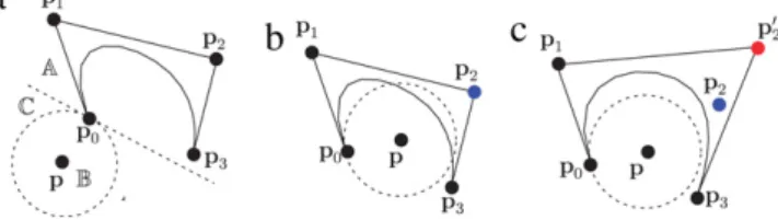
Fig. 2. (a) A curve part can be eliminated with the hyperplane method of [19]. (b) Part of a curve inside a circle, even if all its control points are outside a circle. (c) A curve part can be eliminated with the circular clipping method but not the hyperplane method of [19].

distance function between the test point and a Bézier curve in a Bézier form. In this paper, we first subdivide the NURBS curve into several rational Bézier curves, which may leads to better effi-ciency. Without loss of generality, we may assume that the given curve is a rational Bézier curve. The basic idea is as follows. Sup-pose that point p is a test point, point q is a point on the Bézier curve, and C

(

p

, k

pq

k

)

_{is a circle (or sphere in R}3_{space) with the}

center point p and its radius

k

pq

k

. The nearest point to the point p must be inside the circle C

(

p

, k

pq

k

)

. Thus, any curve part outside the circle C

(

p

, k

pq

k

)

can be directly eliminated. We also call circle

C

(

p

, k

pq

k

)

the elimination circle. During the subdivision process, point q becomes closer and closer to the test point p and the radius of the elimination circle becomes smaller and smaller, which will lead to better elimination efficiency.

One of the key issues for the circular clipping method is to judge whether a curve is outside a circle. If all the control points of a Bézier curve are inside a circle, then the Bézier curve must be inside the circle too. Thus, the elimination circle seems to be useful to compute the maximum distance between a point and a Bézier curve. Unfortunately, even if all the control points of a Bézier curve are outside a circle, we cannot ensure that the Bézier curve is outside the circle (seeFig. 2(b)). It does not seem easy to judge whether a NURBS curve is outside a circle directly by its control polygon. To overcome this problem, we introduce the objective squared distance function for judging whether a curve is outside a circle. Suppose that the curve is q

(

u

)

with its control points

{

p_i

}

p_i=0and the test point is p. From the formula for the product of two B-spline basis function in [25], the objective squared distance function can be rewritten into the following Bézier form

f

(

u

) = (

q

(

u

) −

p

)

2

=

2p

P

i=0

ˆ

Bi,2p

(

u

) ˆw

iP

ˆ

i 2p

P

i=0

ˆ

Bi,2p

(

u

) ˆw

i

.

(2)

From the convex hull property, we obtain the following property.

Property 1. Given

α ∈

R+. If P

ˆ

i

≥

α

, then f

(

u

) ≥ α

, for

∀u

∈

[

0

,

1

]. Thus, the corresponding curve is outside the elimination circle

C

(

p

,

√

α)

.

InProperty 1,

α

denotes the current minimum squared distance between the test point p and the curve q

(

u

)

. Usually, the smaller the value of

α

, the better the elimination efficiency. The initial value of

α

can be simply set to the value min

{k

p₀p

k

2

, k

p_pp

k

2

}

. A fast sampling technique using a forward difference method is quite favorable for selecting a point on the curve q

(

u

)

which is very close to the test point p, which will greatly improve the selection of an initial value of

α

.

We provide a simple termination condition to reduce the subdivision time in the circular clipping algorithm. When the termination condition is satisfied, the minimum value can be robustly solved by directly using the hybrid method of [24] combining binary search and Newton’s method. From the variation

Fig. 3. Efficiency illustration of the new method.

diminishing property, we obtain the following property which presents such a termination condition.

Property 2. If there exists an integer number k

∈ [

1

,

2p

−

1

], such

thatP

ˆ

i

> ˆ

Pi+1, for

∀i

<

k, and thatP

ˆ

i

< ˆ

Pi+1, for

∀i

≥

k. Then f

(

u

)

has exactly one minimum value.

Let Var

(

f

(

u

))

be the variant number of the curve f

(

u

)

, which is defined as the number of sign changes in the sequence

{ ˆ

Pi+1

−

ˆ

Pi

}

m −1

i=0 , where

{ ˆ

Pi

}

are the control points of f

(

u

)

. From the variation

diminishing property of NURBS curve, after a finite number of steps of subdivision, the variant numbers of all the sub-curves of

f

(

u

)

are less than or equal to 1. That is to say, eitherProperty 2

orProperty 1with

α

equal to the squared radius of the clipping circle can be satisfied after a finite number of subdivision steps. WhenProperty 2is satisfied, the hybrid method of [24] combining binary search and Newton’s method is robust for computing the minimum. Thus, both the efficiency and the robustness of the algorithm will be improved by usingProperty 2.

The outline of the circular clipping algorithm mainly has three steps. Firstly, we compute the objective squared distance function in a Bézier form. Secondly, we iteratively subdivide and eliminate the remaining curve parts with the elimination circle with its center point p and its radius

√

α

, until eitherProperty 1with

α

equal to the squared radius of the clipping circle orProperty 2

is satisfied. Finally, the hybrid method of [24] combining binary search and Newton’s method is utilized to compute the locally nearest point as well as its corresponding parameter for each remaining curve part.

3. Analyses and examples

Compared with the root-finding methods, the circular clipping method is able to eliminate most of the roots which do not map to the nearest point. As shown inFig. 1(a)–(c), the squared distance function f

(

u

)

reaches local minimum values at one of the end-points of the curve parts, thus the corresponding curve parts are outside the elimination circle and the corresponding root can be

eliminated. Since the radius of the elimination circle will become smaller and smaller, and part or all of the roots shown inFig. 1(d) can be eliminated (also seeFig. 3(b)).

We also compare the new method with the geometric exclusion methods based on the subdivision of the NURB curve. The control polygon method of [2] is efficient for curves in R2_{space. However,}

it may fail for curves in R3 _{space [20]. We compare the circular}

clipping method with the hyperplane clipping method. First of all, the exclusion criteria of our method utilizes a considerably larger clipping area than the criteria of [19]. As shown inFig. 2(a), the hyperplane clipping method of [19] eliminates the curve parts inside region A, while the circle clipping method may eliminate the curve parts inside both regions A and C.

Next, as shown in Fig. 3, the circular clipping method can remove more unnecessary parameter intervals than the hyperplane clipping method of [19]. InFig. 3(a), p is a test point,

{

p_i

}

4

i=0are control points of a NURBS curve. In this case, the curve

is outside the elimination circle C

(

p

, k

pp₀

k

)

and the exclusion criteria in the new method is satisfied. However, since

(

p₄

−

p₀

)(

p₀

−

p

) <

0, the exclusion criteria in [19] is not satisfied. In Fig. 3(b), the shape of the NURBS curve is complicated. After subdividing the curve, we obtain two sub-curves, one is in black, and the other is in red. The exclusion criteria in [19] is still not satisfied for both sub-curves. The sub-curve in red is outside the elimination circle C

(

p

, k

pp₀

k

)

and can be removed by the circular clipping method.

Again, there are much fewer subdivision steps in the circular clipping method than those in the hyperplane method of [19], which can lead to better efficiency in the new method. For NURBS curves in Rd_{space, though the computation time of each}

subdivision step in the circular clipping method is about 4

/

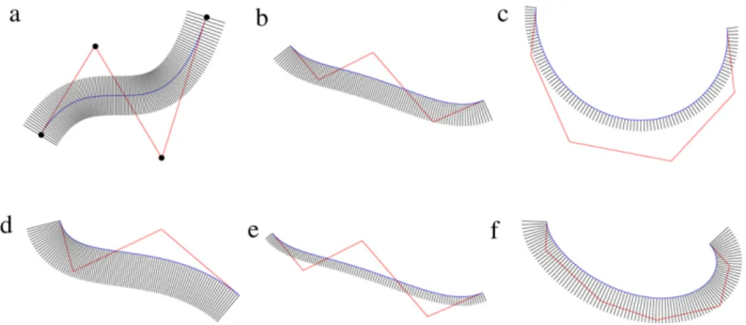
d times

of that in the hyperplane clipping method, the total computation time on subdivision in the new method is much less than that in the hyperplane clipping method.Fig. 4shows three non-rational cases and three rational cases. And the test points are sampled along their offset curves. We compare the new method with the methods in [2,19] by using these examples. The corresponding results are shown inTable 1. Both the subdivision time and the computation time of the new method is less than those of the other two methods. And the computation time in [19] is the most expensive among the three methods. However, in the circular clipping method, there is an extra computation time on obtaining the objective squared distance function determined by Eq.(2)in a Bézier form.

Finally, the Newton method in the hyperplane clipping method of [19] needs a good initial value and its resulting efficiency and accuracy are very sensitive to the given tolerance for ter-minating the subdivision process. On the other hand, the circu-lar clipping method works less sensitively to the initial value and

Fig. 4. Examples. (a) A cubic Bézier curve (b) a quartic Bézier curve (c) a quintic Bézier curve (d) a cubic rational Bézier curve (e) a quartic rational Bézier curve (f) a sextic rational Bézier curve.

1054 X.-D. Chen et al. / Computer-Aided Design 40 (2008) 1051–1054

Table 1

Comparison on subdivision time and computation time

Subdivision time Computation time

Method Ma Selimovic Ours Ma (ms) Selimovic (ms) Ours (ms)

Fig. 4(a) 5.55 18.8 0.14 0.020 0.634 0.004 Fig. 4(b) 6.29 24.33 0.38 0.024 2.414 0.010 Fig. 4(c) 6.06 26.62 0.35 0.027 3.112 0.014 Fig. 4(d) 6.15 19.5 0.31 0.024 0.784 0.018 Fig. 4(e) 7.23 27.34 1.0 0.046 3.103 0.027 Fig. 4(f) 9.36 35.62 2.2 0.078 5.418 0.053

Fig. 5. Correctness comparison. (a) A quartic Bézier curve. (b) Resulting closest points from the method of Ma and Hewitt [2] and the method of Selimovic [19]. (c) Resulting closest points from the circular clipping method.

ensures convergence to an accurate result.Fig. 5shows such an example. Fig. 5(a) shows a quartic Bézier curve with its con-trol points

(−

3

.

6164

, −

18

.

7790

)

T_,

₍

₃

_.

₇₈₀₈

_,

₂₆

_.

₅₀₇₀

₎

T_,

₍₋

₀

_.

₆₅₇₅

_,

−

45

.

9815

)

T_,

₍₋

₂

_.

₂₃₅₃

_,

₄₄

_.

₁₂₆₇

₎

T_,

₍

₁₇

_.

₁₇₆₅

_{, −}

₁

_.

₄₆₈₃

₎

T_{, and the}

test points are sampled along the circle with its radius 0.1340 and its center point

(

0

.

5057

, −

2

.

4590

)

T_{.Fig. 5(b) and (c) magnify the}

local region framed by a green rectangle. The lines are drawn from the test points to the corresponding closest points on the Bézier curve. The results from the method of Ma and Hewitt [2] and the method of Selimovic [19] are similar as shown inFig. 5(b). In

Fig. 5(b), the lines in red denote incorrect results from these two methods, the corresponding lengths of which are 0.1341, 0.1327 and 0.1209, respectively.Fig. 5(c) shows the result from the circu-lar clipping method, where the corresponding lines in green are of lengths 0.1296, 0.1092 and 0.0909, respectively. It shows that the circular clipping method is more robust than the methods in [2,19].

4. Conclusions

This paper presents a circular clipping method for computing the minimum distance between a point and a NURBS curve. Com-pared with the root-finding methods, the new method can elimi-nate most of the roots of Eq.(1)and reduce most of the computa-tion time on solving the roots. Compared with other comparable geometric methods in [2,19], the new method can eliminate more curve parts and has better robustness. Examples are shown to il-lustrate the efficiency and robustness of the new method.

Acknowledgements

The research was partially supported by Chinese 973 Program (2004CB719400), the National Science Foundation of China (60803076,60625202,60473130), INRIA, Chinese 863 Program (2007AA040401) and the Open Project Program of the State Key Lab of CAD&CG (A0804), Zhejiang University. The second author was supported by a Foundation for the Author of National Excellent Doctoral Dissertation of PR China (200342) and Fok Ying Tung Education Foundation (111070). The authors would like to thank the reviewers and Professor Wenping Wang for their helpful comments.

References

[1] Hu SM, Wallner J. A second order algorithm for orthogonal projection onto curves and surfaces. Computer Aided Geometric Design 2005;22(3):251–60.

[2] Ma YL, Hewitt WT. Point inversion and projection for NURBS curve and surface: Control polygon approach. Computer Aided Geometric Design 2003;20(2): 79–99.

[3] Yang HP, Wang WP, Sun JG. Control point adjustment for B-spline curve approximation. Computer-Aided Design 2004;36:639–52.

[4] Johnson DE, Cohen E. A framework for efficient minimum distance computa-tions. In: Proceedings of IEEE intemational conference on robotics & automa-tion. 1998. p. 3678–84.

[5] Piegl L, Tiller W. Parametrization for surface fitting in reverse engineering. Computer-Aided Design 2001;33(8):593–603.

[6] Pegna J, Wolter FE. Surface curve design by orthogonal projection of space curves onto free-form surfaces. Journal of Mechanical Design, ASME Transactions 1996;118(1):45–52.

[7] Besl PJ, McKay ND. A method for registration of 3-D shapes. IEEE Transactions on Pattern Analysis and Machine Intelligence 1992;14(2):239–56.

[8] Mortenson ME. Geometric modeling. New York: Wiley; 1985.

[9] Zhou JM, Sherbrooke EC, Patrikalakis N. Computation of stationary points of distance functions. Engineering with Computers 1993;9(4):231–46. [10] Johnson DE, Cohen E. Distance extrema for spline models using tangent cones.

In: Proceedings of the 2005 conference on graphics interface. 2005. [11] Gutierrez JM, Hernandez MA. An acceleration of Newton’s method:

Super-Halley method. Applied Mathematics and Computation 2001;117(2):223–39. [12] Polak E. Optimization, algorithms and consistent approximations. Berlin

(Heidelberg, NY): Springer-Verlag; 1997.

[13] Polak E, Royset JO. Algorithms with adaptive smoothing for finite minimax problems. Journal of Optimization : Theory and Applications 2003;119(3): 459–84.

[14] Press WH, Teukolsky SA, Vetterling WT, Flannery BP. Numerical recipes in C: The art of scientific computing. 2nd ed. New York: Cambridge University Press; 1992.

[15] Elber G, Kim MS. Geometric constraint solver using multivariate rational spline functions. In: Proceedings of the sixth ACM symposium on solid modeling and applications. 2001. p. 1–10.

[16] Patrikalakis N, Maekawa T. Shape interrogation for computer aided design and manufacturing. Springer; 2001.

[17] Sederberg TW, Nishita T. Curve intersection using Bézier clipping. Computer-Aided Design 1990;22(9):538–49.

[18] Chen XD, Zhou Y, Shu ZY, Su H, Paul JC. Improved algebraic algorithm on point projection for Bézier curves. In: International multi-symposiums on computer and computational sciences. USA: The University of Iowa; 2007.

[19] Selimovic I. Improved algorithms for the projection of points on NURBS curves and surfaces. Computer Aided Geometric Design 2006;23(5):439–45. [20] Chen XD, Su H, Yong b JH, Paul JC, Sun JG. A counterexample on point inversion

and projection for NURBS curve. Computer Aided Geometric Design 2007;24: 302.

[21] Boehm W. Inserting new knots into B-spline curves. Computer-Aided Design 1980;12:199–201.

[22] Cohen E, Lyche T, Riesebfeld R. Discrete B-splines and subdivision techniques in computer-aided geometric design and computer graphics. Computer Graphics and Image Processing 1980;14:87–111.

[23] Piegl L, Tiller W. The NURBS book. New York: Springer; 1995.

[24] Ye Y. Combining binary search and Newton’s method to compute real roots for a class of real functions. Journal of Complexity 1994;10(3):271–80. [25] Morken K. Some identities for products and degree raising of splines.