Algorithms Above The Noise Floor
by
Ludwig Schmidt
Submitted to the Department of Electrical Engineering and Computer Science
in partial fulfillment of the requirements for the degree of
Doctor of Philosophy
at the
MASSACHUSETTS INSTITUTE OF TECHNOLOGY
June 2018
Ludwig Schmidt, MMXVIII. All rights reserved.
The author hereby grants to MIT permission to reproduce and to distribute publicly
paper and electronic copies of this thesis document in whole or in part in any
medium now known or hereafter created.
Signature redacted
A uthor ...
...
Department of Electrical Engineering and Computer Science
May 23, 2018
Signature redacted
C ertified by ...
...
Piotr Indyk
Professor of Electrical En ineering and Computer Science
Thesis Supervisor
Signature redacted
A ccepted by ...
...
/
6
U Leslie A. Kolodziejski
Professor of Electrical Engineering and Computer Science
Chair, Department Committee on Graduate Students
MASSACHUSETTS INSTIUTE
OF TECHNOLOGY
JUN 18.2018
LIBRARIES
ARCHIVE$
Algorithms Above The Noise Floor
by
Ludwig Schmidt
Submitted to the Department of Electrical Engineering and Computer Science on May 23, 2018, in partial fulfillment of the
requirements for the degree of Doctor of Philosophy
Abstract
Many success stories in the data sciences share an intriguing computational phenomenon. While the core algorithmic problems might seem intractable at first, simple heuristics or approximation algorithms often perform surprisingly well in practice. Common examples include optimizing non-convex functions or optimizing over non-convex sets. In theory, such problems are usually NP-hard. But in practice, they are often solved sufficiently well for applications in machine learning and statistics. Even when a problem is convex, we often settle for sub-optimal solutions returned by inexact methods like stochastic gradient descent. And in nearest neighbor search, a variety of approximation algorithms works remarkably well despite the "curse of dimensionality".
In this thesis, we study this phenomenon in the context of three fundamental algorithmic problems arising in the data sciences.
* In constrained optimization, we show that it is possible to optimize over a wide range of non-convex sets up to the statistical noise floor.
" In unconstrained optimization, we prove that important convex problems already
require approximation if we want to find a solution quickly.
* In nearest neighbor search, we show that approximation guarantees can explain much of the good performance observed in practice.
The overarching theme is that the computational hardness of many problems emerges only below the inherent "noise floor" of real data. Hence computational hardness of these problems does not prevent us from finding answers that perform well from a statistical perspective. This offers an explanation for why algorithmic problems in the data sciences often turn out to be easier than expected.
Thesis Supervisor: Piotr Indyk
Title: Professor of Electrical Engineering and Computer Science
To my parents
Acknowledgments
First and foremost, I want to thank my advisor Piotr Indyk. Starting graduate school without much research experience, I was initially quite uncertain which direction to pursue. Deciding to work with Piotr turned out to be an excellent choice in many ways. Piotr was always supportive of my interests at the intersection of theory and practice and introduced me to many problems of this flavor. The direction he put me on turned out to be a perfect combination of my background in combinatorial algorithms with my interests in machine learning. Along the way, I learned a lot from Piotr's quick insights and vast knowledge of algorithms. Piotr was always supportive of my career and generously kept me free from worries about funding. Finally, Piotr is a remarkably kind person and truly cares about his students, which made his research group a pleasure to be in.
Next, I want to thank Chinmay Hegde. Chin came to MIT as a postdoc at the beginning of my second year and effectively became my co-advisor. Chin taught me many topics in signal processing, which was invaluable to get started with my research. Over the years, we developed both a very fruitful research collaboration and a good friendship. Almost all of my early papers are co-authored with Chin, and my work with Piotr and Chin forms the core of this thesis.
In the middle of my PhD, I benefited from the guidance of four mentors. Ben Recht and Martin Wainwright were very welcoming when they hosted me at Berkeley in Spring
2016. The following two summers (and part-time in between), I was lucky to intern with
Yoram Singer and Kunal Talwar at Google Brain. Talking to Ben, Kunal, Martin, and Yoram broadened my perspective beyond the core algorithmic problems I had worked on and prompted me to think more deeply about statistics and machine learning. This had a lasting (and very positive!) effect on my research and significantly influenced this thesis. The final year of my PhD was not entirely planned and arguably correlated with the fact
that I began working with Aleksander Mqdry. It turned out that Aleksander was about to launch a research program that aligned very well with my interests and led me to many fascinating problems (which more than compensate for the repeatedly delayed thesis defense!). Moreover, Aleksander has been a great mentor over the past year and I am very grateful for his support.
Besides Aleksander and Piotr, my third committee member is Costis Daskalakis, who was also part of my RQE committee. I would like to thank Costis for his input, encouraging words, and being flexible with the timeline of this thesis.
A very important part of my PhD are my collaborators. Over the past seven years, I was
fortunate to join many colleagues in research projects. Listing all of them (more than 40) would go beyond the limits of these acknowledgements, but I am very grateful to each of them. You taught me many topics through our collaborations and I truly enjoyed the company. Thank you!
However, I can't get around mentioning two student collaborators. Jerry Li has been the perfect companion for my ventures into learning theory. I learned a lot from Jerry's math background, and I hope I didn't do too much damage by adding experiments to our papers. The other student who influenced my work significantly is Michael Cohen, who tragically passed away during the last year of my PhD. Talking to Michael has been one of the greatest
intellectual privileges during my time at MIT, and also one of the biggest sources of fun conversations. It is impossible to do justice to Michael in a few sentences. I can just say that I truly miss him.
Beyond the academic side of graduate school, I was lucky to be part of many great commu-nities at MIT. The theory group has been an excellent place not only for work but also for companionship (thanks for organizing, G!). I lived in Ashdown House during my entire time at MIT, which was always a welcoming home to come back to outside the department. The MIT Outing Club (MITOC) has been an incredible community for my outdoor activities.
My friends at MITOC introduced me to all varieties of hiking and brought me to
moun-tains that I would have never climbed alone. Thank you (among many others) Anthony, Ben, Elliott, Eric, Katherine, Katie, Maddie, Margie, Matthew, Meghan, Michele, MinWah, Nathaniel, Rachel, Richard, Rob, Vlad and Yuval!
Over the past few years, I was fortunate to meet many wonderful friends at MIT, Berkeley, and beyond. I am surely forgetting some important names (sorry!), but I would still like to mention a few friends individually: Adam, Alex, Alison, Arturs, Christos, Fanny, Fredrik, Henry, Madars, Maithra, Matt, Reinhard, Philipp, Ruby, and Ryan: thank you for all the great time together and supporting me throughout grad school!
An important milestone on the way to MIT were my undergrad years at Cambridge. My directors of study at Trinity, Arthur Norman and Sean Holden, gave me plenty of freedom and helped me get into MIT. I also learned a lot from my friends Ada, Freddie, Martin, Rasmus, and Sean, who - together with many others - provided great company over the years. I'd especially like to thank Felix Arends, who was always a few years ahead of me and inspired me to go to Cambridge and then to intern at Google.
While my school days are a while in the past now, it is clear that I would not be here without the early support from that time. My high school teachers Helmut Eckl, Alois St6hr, and Stefan Winter got me started with math and computer science competitions early, which put me on a trajectory that I continue to benefit from. The most influential competition for me has been the Bundeswettbewerb Informatik (BWInf). Together with the informatics olympiads, it shifted my focus from mathematics to computer science. The BWInf and the German olympiad team are still organized by Wolfgang Pohl, who I am very grateful to. I would also like to thank the "Schiilerstudium" team at the University of Passau for giving me an early start with studying computer science. And school would have been boring without my friends: Andreas, Andreas, Henry, Johannes, Julian, Matthias, Max, Simon, Simon, Simon, Stephan (and everyone I can't list here right now) - thank you for all the good times!
Finally, I would like to thank my family. My brother Valentin has kept me grounded over the years and has always been a great source of fun and laughter. My parents, Barbara and Norbert, have supported me in everything I wanted to do, and I could not be more grateful for that. This thesis is dedicated to them.
Contents
Contents 9
1 Introduction 11
I Optimizing Over Non-Convex Cones 21
2 Projected gradient descent for non-convex cones 23
3 Graph sparsity 63
4 Group sparsity 107
5 Tree sparsity 119
6 Earth Mover Distance sparsity 167
7 Low-rank matrices 185
8 Histograms 195
II Lower Bounds for Unconstrained Optimization 210
9 The fine-grained complexity of empirical risk minimization 211
III Nearest Neighbor Search 241
10 Unifying theory and experiment in locality-sensitive hashing 243
11 Learning embeddings for faster nearest neighbor search 263
Bibliography 281
Chapter 1
Introduction
Over the past two decades, the reach of data sciences such as machine learning, statistics, and signal processing has grown tremendously. Fueled by our ever-increasing capabilities to collect large amounts of data, statistical algorithms now underlie a broad range of modern technology. Well-known examples include web search, medical imaging, bioinformatics, computer vision, and speech recognition - just to name a few. From a computational perspective, many of these success stories highlight an intriguing overarching theme: while the core algorithmic problems might seem costly to solve or even intractable at first, simple heuristics or approximation algorithms often perform surprisingly well in practice.
Examples of this phenomenon are abundant. In statistical estimation tasks, it is now standard practice to optimize over non-convex sets (e.g., sparse vectors or low-rank matrices), even though such problems are NP-hard in general. When training neural networks or fitting random forests, iterative methods often find good solutions in spite of the non-convex loss functions. Even for convex problems, we commonly resort to stochastic gradient methods that return only coarse answers yet still provide good generalization properties. And when searching through large collections of complex data such as images or videos, approximate data structures quickly return the right answer in spite of the "curse of dimensionality". This discrepancy between the inexact nature of popular algorithms and their good empirical performance raises a fundamental question:
When and why do approximate algorithms suffice in statistical settings?
There are multiple reasons to study this question. On the theoretical side, we should understand how statistical settings evade fundamental hardness results. After all, the hallmark of a scientific theory is its predictive power. But when it comes to predicting performance in machine learning or statistics, the dominant "worst case" view of algorithms often seems too pessimistic.
On the more applied side, the growing influence of data sciences also means that errors made by our algorithms can have direct negative consequences in the real world. If we want to responsibly utilize these algorithms in scenarios with serious impact, it is important to delineate the regimes where we can safely rely on their answers. Finally, understanding why inexact solutions work well often enables us to develop new algorithms that achieve even better computational or statistical performance.
The goal of this thesis is to explain and extend the success of approximate algorithms in statistical settings. To this end, we investigate three fundamental algorithmic problems in the data sciences. All three vignettes share a common theme: approximate algorithms consistently avoid computational hardness results, but still achieve strong performance both in theory and in practice.
At a high level, our results show that the computational hardness of many algorithmic problems only emerges when we compute high-accuracy solutions below the inherent "noise floor" of the data we collected. So from the perspective of the statistical problem we want to solve, the computational hardness of the intermediate algorithmic problem often turns out to be irrelevant. This explains why algorithmic problems in the data sciences can usually be solved sufficiently well in practice, even if a worst case perspective might at first suggest otherwise.
The work in this thesis makes contributions to the following areas:
Constrained optimization. Optimizing over convex sets is a well-understood task with polynomial-time algorithms for a broad range of constraints. In contrast, even simple
problems involving non-convex sets are NP-hard. Nevertheless, seminal results in compressive sensing show that statistical settings improve the situation markedly. For certain non-convex sets such as sparse vectors and low-rank matrices, we now have reliable algorithms and a comprehensive understanding of both computational and statistical aspects. But the situation is still less clear for general non-convex sets. In this thesis, we introduce an extension of projected gradient descent for arbitrary non-convex cones that achieves (near-) optimal statistical accuracy. Moreover, we identify a new notion of approximately projecting onto non-convex sets. This notion allows us to optimize over constraints that would otherwise be NP-hard to handle. In addition to their strong theoretical guarantees, our algorithms also improve over the state of the art in numerical experiments.
Unconstrained optimization. Stochastic gradient descent (SGD) is a ubiquitous
algo-rithm in machine learning and underlies many successful classification techniques. On the one hand, research has shown that SGD returns solutions with good statistical properties. On the other hand, SGD relies on approximate gradients and has only modest convergence guarantees as an optimization algorithm. As a result, SGD is often unreliable and requires instance-specific tuning of hyperparameters. Such brittle performance is a common hidden cost of approximate algorithms. So why do we resort to sometimes unreliable algorithms?
To explain our dependence on approximate algorithms, we show that computational limits already emerge when solving important convex problems to high accuracy. Two concrete examples in this thesis are kernel support vector machines (SVM) and kernel ridge regression, which are widely used methods in machine learning. For these problems, a reliable high-accuracy algorithm with subquadratic running time would break a well-established barrier in complexity theory. So our use of inexact algorithms like SGD is probably due to the fact that there is no "silver bullet" algorithm for these problems. There are inherent computational limits when working with powerful data representations such as kernels. This shows that the negative side effects of approximate algorithms are sometimes unavoidable.
Nearest neighbor search. Quickly searching through vast amounts of data plays a key
role in important technologies such as web-scale search engines and recommender systems. However, there are (conditional) lower bounds telling us that fast nearest neighbor search should be impossible in general. So what structure in the data do successful algorithms exploit? The Locality Sensitive Hashing (LSH) framework provides a rigorous explanation. But empirically, LSH lost ground to other methods over the past decade.
In this thesis, we bridge this divide between theory and practice and re-establish LSH as a strong baseline. We thereby demonstrate that the LSH theory can explain much of the good performance observed in practice. Moreover, we show empirically that the assumptions in the LSH theory are naturally satisfied when the dataset is derived from a trained embedding such as a neural network. On the practical side, our LSH implementation FALCONN has become a popular library for nearest neighbor search on GitHub.
In the next three sections, we outline our concrete contributions in more detail. At a high level, each part of this thesis corresponds to one of the three algorithmic problems mentioned above.
1.1
Optimizing over non-convex cones
The goal in constrained optimization is to minimize an objective function
f :
Rd -+ R over a given constraint set C C Rd. This fundamental paradigm has found a myriad of applicationsand has led to influential algorithmic techniques such as the simplex algorithm or interior point methods. The classical theory of optimization shows that for a broad range of convex constraint sets, it is possible to solve constrained optimization problems in polynomial time (for instance, linear programs or semidefinite programs) [40, 54, 174, 175]. Building on this work, a large body of research from the past 15 years has focused on applications with
non-convex constraints. Here, the situation is more subtle. Even simple problems over
non-convex sets can be NP-hard, yet are often solved successfully in practice.
One important example in the data sciences are estimation problems. In a linear estima-tion problem, we want to (approximately) recover an unknown parameter vector 0* E Rd from a small number of linear observations. We can summarize n such observations in a measurement matrix X E Rnxd and a response vector y E
R'
to get the following data model:y = X0*
+
e,where e E R' is an unknown noise vector. Since this is a linear model, a natural approach to estimating 0* is a constrained least squares problem of the form
minimize
Iy
- X01|| subject to 0 E C .In this formulation, the constraint set C encodes our prior knowlege about the unknown parameters 0* (e.g., a sparsity or rank constraint). While the linear setup might seem simple at first, it already applies to a broad range of problems including magnetic resonance imaging
[157], recommender systems [59], and selecting important features in gene expression data
[222]. In these applications, utilizing prior knowledge through carefully chosen constraints is crucial for finding a good estimate from a small number of samples.
From a worst case perspective, Problem (1.1) might seem hopeless. For instance, the least squares problem is already NP-hard for simple non-convex constraints such as C being the set of sparse vectors [168]. Nevertheless, various algorithms often find good estimates in practice [73, 221]. To explain this phenomenon, the fields of compressive sensing and high-dimensional statistics have developed a rich theory for optimizing over certain non-convex sets [69, 101, 114, 231]. Under regularity assumptions on the matrix X, corresponding algorithms provably find an estimate 0 such that 0 ~ 0* up to the inherent noise in the problem.
At a high level, there are two algorithmic approaches to estimating 0*:
* Convex relaxations relate the non-convex constraint back to a convex counterpart. The
statistical guarantees for estimating 0* are well understood and in many cases optimal. While this approach has been very successful for some non-convex constraints (e.g., sparse vectors and low-rank matrices [59, 60, 90, 186]), it is not clear how to derive convex relaxations for other constraint sets (e.g., graph sparsity or group sparsity
[232]).
* Projected gradient descent (PGD) forgoes the convex route and directly works with the non-convex set. While this succeeds for well-conditioned problems [50, 80, 131, 170,
177], the PGD approach does not match the sample complexity of convex relaxations
in the general case [133]. Moreover, PGD relies on access to an efficient projection
oracle for the non-convex set C.1 Unfortunately, the projection problem can also be NP-hard (among others, the culprits are again graph sparsity and group sparsity [33,
118]). In such cases, PGD does not have a polynomial running time.
Methods for sparse vectors and low-rank matrices have been highly successful despite the non-convex constraints. Hence it is important to understand how general this phenomenon is. Specifically, we investigate the following question:
For what non-convex sets can we solve constrained estimation problems efficiently?
In this thesis, we significantly extend the class of non-convex sets for which we can efficiently optimize in a statistical setting. In particular, we make the following three contributions:
Result 1. We introduce a generalized version of projected gradient descent for
non-convex sets that achieves the optimal sample complexity for estimation problems with arbitrary conditioning.
This result provides an alternative path to optimal statistical performance that does not rely on convex relaxations. However, the new algorithm still relies on projections for the set C, which can be an NP-hard sub-problem. To ameliorate this issue, we show that our generalization of PGD also works when combined with a weaker notion of projection.
Result 2. Our generalized PGD algorithm still succeeds when it only has access to
approximate projections.
While PGD has been combined with approximate projections before [39, 49, 82, 107, 108, 144, 145, 205], our framework is the first that leads to faster algorithms for a broad range of constraint sets. An important insight is that we need to combine PGD with two comple-mentary notions of approximate projections simultaneously.
To instantiate our new PGD framework, we have to provide approximate projections for concrete constraint sets. To this end, we combine ideas from both continuous and dis-crete optimization. Our faster projections leverage a broad range of techniques from the approximation algorithms literature.
Result 3. We exhibit many constraint sets for which an approximate projection is provably faster than an exact projection.
This result summarizes multiple independent algorithms in this thesis. Among others, we give fast approximate projections for constraint sets defined by low-rank matrices, hierar-chical sparsity, graph sparsity, group sparsity, and k-histograms (see Table 2.1 for details). Even in cases where an exact projection is NP-hard (such as graph sparsity and group sparsity), we can still approximately project in nearly-linear time.
Our three results show that we can optimize over a diverse collection of non-convex sets as long as we stay above the noise floor of the estimation problem. In particular, approximate projections provide a concrete new example of algorithmic problems that become significantly easier in a statistical setting. Although they solve the intermediate projection problems only approximately, they still provide optimal statistical guarantees in the overall estimation task. Our provable guarantees also show how PGD-like heuristics can succeed in practice even when applied to non-convex sets. Finally, we remark that our algorithms improve over prior work both in theory and in experiments.
1.2
Lower bounds for unconstrained optimization
Another large class of algorithmic problems arising in the data sciences are instances of unconstrained optimization. One important framework here is empirical risk minimization (ERM) [225]. For a set of labeled data points (Xi, y1),..., (Xn, yn) and a loss function L, the goal is to find a minimizer 0 of the empirical risk
n
La(6) = L(0, xi, yi).
The loss function L encodes how well the parameters 0 fit the data point (X, y). By varying the loss function and the underlying classifier, the ERM paradigm encompasses widely used learning techniques such as logistic regression, support vector machines (SVM), and artificial neural networks [207].
Over the past decade, stochastic gradient descent (SGD) has emerged as a powerful tool for approximately solving ERM problems [52, 188]. The main idea of SGD is to work with
approximate gradients obtained from only a subset of the data points in each iteration (as
opposed to the exact gradient from all n data points). Especially for large datasets, a single iteration of SGD can be multiple orders of magnitude faster than a single iteration of gradient descent.
For convex ERM problems (and some non-convex ones), it is now understood that SGD quickly finds solutions that generalize, i.e., achieve good classification accuracy on new unseen data [113, 173, 180]. Nevertheless, the approximate gradients used in SGD come at a cost. While they allow the algorithm to make rapid initial progress, SGD only converges slowly to the true minimizer of the empirical risk. This leads to the following issues:
. It is often unclear if a low classification accuracy is a failure of optimization (e.g., an inaccurate ERM solution) or learning (wrong choice of model or insufficient data). . Achieving good performance with SGD often requires fine-tuning various parameters
such as the step size [239].
* Seemingly benign questions such as step size schedules or adaptive step size selection are still the subject of current research and actively debated in the community [94,
141, 187, 216, 239].
This unreliable behavior of SGD can add significant overhead to the overall training time. It also limits the effective use of machine learning to a small number of expert researchers. In contrast to SGD, an ideal algorithm should reliably and quickly converge to the empirical risk minimizer. The fact that we are stuck with tuning SGD raises a natural question:
What are the fundamental computational limits of empirical risk minimization?
The second part of our thesis addresses this question in both convex and non-convex settings.
Convex ERM. How would an ideal ERM algorithm look like? Formally, our goal is to find an e-approximate solution to the ERM problem, i.e., an estimate 0 that is e-close to an optimal solution
0*:
Ln($) - Ln(O*) < E .
An ideal algorithm would have a time complexity of 0 (n log 1/F). This running time implies that the algorithm would return a high-accuracy solution (due to the log 1/e dependence) with only a small cost per iteration (the linear dependence on n). Note that it is possible to achieve both goals individually. So-called interior point methods have a log 1/e dependence but usually require expensive iterations with a cost of 0(n3) [40, 54, 174, 175]. In constrast, SGD has cheap iterations but only a slow convergence rate where the accuracy parameter
enters as 1/e (without the logarithm) [208]. Is it possible to achieve the best of both worlds? We utilize results from fine-grained complexity to show that such an ideal algorithm is probably impossible for two important ERM problems. In particular, we build on the
Strong Exponential Time Hypothesis (SETH), which can be seen as a natural strengthening
Result 4. Assuming SETH, no algorithm can solve kernel support vector machines
and kernel ridge regression to high accuracy in subquadratic time.
From a practical perspective, a quadratic running time can be burdensome or even prohibitive for datasets with n = 106 or n - 10' data points, which are now increasingly common.
So unless a new algorithm cleverly exploits extra problem-specific structure, we have to live with the downsides of approximate algorithms for large datasets. This shows that our reliance on approximations in statistical settings is not only a matter of convenience but due to fundamental computational limits. Moreover, our result justifies the use of SGD and other approximation methods (e.g., random features or the Nystr6m method [179, 234]) for large-scale kernel problems.
Non-convex ERM. Finding the exact minimizer of the empirical risk is NP-hard even for simple non-convex problems [47]. But in practice, SGD has become a surprisingly effective tool for non-convex problems such as training neural networks. While the success of SGD is not yet well understood, can we give evidence that SGD - as currently employed - is in some sense optimal?
When we run SGD to train a large neural network, the main computational burden is computing the gradient of the loss with respect to the network parameters. This is the problem commonly solved by the seminal backpropagation algorithm that is now implemented in all major deep learning frameworks [195]. The standard approach is to compute gradients for a batch of examples and then to update the network parameters with the average gradient. Since data batches now contain hundreds or even thousands of data points, it is important to understand how quickly we can compute batch gradients [111].
For a neural network with p hidden units, computing the gradient of a single data point via backpropagation takes
0(p)
time. With a batch of size n, the standard approach is to simply compute the gradient of each data point individually and then to average the result. This has a rectangular time complexity ofO(n
- p). But from an information-theoreticperspective, the algorithm has all the information for computing the batch gradient after reading the input (the network and the data points) in time O(n + p). So is it possible to improve over the rectangular running time? We again leverage the fine-grained complexity toolkit to prove that the rectangular running time is (likely) optimal.
Result 5. Assuming SETH, approximately computing the gradient of a two-layer network with rectified linear units (ReLU non-linearities) requires O(n -p) time.
Our hardness result suggests that it may be impossible to significantly improve over back-propagation for computing gradients in neural networks. As in kernel methods, this perspec-tive points towards an inherent tension between the representational power of a learning approach and the resulting computational hardness. Furthermore, our result provides an explanation for why backpropagation has been an unchanged core element in deep learning since its invention.
1.3
Nearest neighbor search
The third algorithmic problem we focus on is nearest neigbor search (NNS). Given a dataset of d-dimensional points P = {pl,. . ., p,} and a distance function 6 : Rd x Rd -+ R, we first build a data structure that then allows us to answer nearest neighbor queries efficiently. Specifically, for a given query point q E Rd, our goal is to quickly find its nearest neighbor
arg min 6(p,q) pEP
NNS is a fundamental tool for processing large datasets and is commonly used for exploratory
data analysis and near-duplicate detection. Moreover, large-scale recommender systems and search engines rely on NNS as an integral component.
A simple baseline for NNS is a linear scan: when a new query q arrives, simply compute
the distance 6(pi, q) to all n points without building a data structure beforehand. We then pick the closest point pi, which can be done in 0(n) total time. In fact, this baseline is (nearly) optimal in the general case: there are conditional lower bounds proving that a strongly sub-linear query time is impossible [15, 84, 192, 235]. But as datasets continue to grow, it is increasingly important to design fast algorithms with a sublinear query time. Indeed, there is now a long line of work on data structures for NNS that enable fast query times in practice. Popular examples include k-d trees [41], Locality Sensitive Hashing (LSH) [112, 127], product quantization [134], and graph-based approaches [159]. Their impressive empirical performance raises a natural question:
Why do nearest neighbor algorithms work well in practice?
The theory of LSH offers an explanation via distance gaps. To be concrete, let us assume that the query point q is c times closer to its nearest neighbor p* than to all other data points. We can formalize this as
(qp*) <; - .6(q,p) for p E P \ {p*}. C
Intuitively, large distance gaps should lead to an easier nearest neighbor problem since there is more "contrast" between the nearest neighbor and an average data point. Indeed, the seminal hyperplane hash yields a data structure with query time 0(n'/C) for the widely used angular distance (also known as cosine similarity) [70]. This sublinear query time is responsible for the good empirical performance of the hyperplane hash. It also shows how the linear time hardness of NNS only appears below the "noise floor" given by the distance
gaps.
However, more recent NNS techniques have improved significantly and now outperform the hyperplane hash by an order of magnitude on standard benchmarks [23, 43]. So are distance gaps still sufficient to explain the good performance of NNS methods in practice? And even if distance gaps still suffice, it is not clear why a dataset would have large distance gaps to begin with. This thesis addresses both of these questions.
Bridging theory and practice of locality-sensitive hashing. Can distance gaps provide faster query times than the 0(n/c) achieved by the hyperplane hash? Over the
past decade, theoretical research has shown that more advanced hash functions achieve a 0(nl/2) query time [16, 18, 19]. The quadratically better exponent could potentially lead to faster query times in practice as well. But unfortunately, this has not happened so far. The main bottleneck of the theoretically motivated hash functions is the time it takes to compute the hash function itself. Here, a key feature of the hyperplane hash becomes apparent: computing a single hash function costs only 0(d) time, while the theoretically better hash functions have higher time complexities such as 0(d2
). Is it possible to combine the good sensitivity (i.e., small query time exponent) of more advanced hash functions with the fast computation time of the hyperplane hash?
Our starting point is the cross-polytope (CP) hash originally introduced by Terasawa and Tanaka [219]. The authors conduct insightful experiments demonstrating that the CP hash has a good sensitivity. But they do not provide theoretical proofs for this phenomenon. Moreover, their version of the CP hash also suffers from the slow 0(d2
) time to compute a hash function and consequently was not adopted in practice. Our work addresses these shortcomings. A key ingredient are ideas from randomized dimensionality reduction that enable us to compute the CP hash in 0(dlogd) time [12].
Result 6. The cross-polytope hash provably achieves a 0(nl/2) query time in the locality-sensitive hashing framework. Empirically, it also improves over the hyperplane hash by a factor of 4x to 10x for datasets of size 106 to 108.
We converted our research implementation of the CP hash into an open source library called FALCONN [185].1 When we released FALCONN in 2015, it was the fastest library in the standard NNS benchmark and improved over the prior state-of-the-art by a factor 2x to 3x [43]. Moreover, it was the first LSH-based technique that empirically improved over the hyperplane hash in more than a decade. While a graph-based approach surpassed
FALCONN in the following year, our library is still competitive with the state-of-the-art [23]. This demonstrates that distance gaps can indeed provide a good explanation for the
empirical success of NNS. Moreover, FALCONN has become a popular library on GitHub and found users in both academia and industry [185].
Understanding distance gaps in learned embeddings. LSH explains how distance
gaps enable fast NNS in practice. But where do these distance gaps come from? In the past, feature vectors for images, text, or speaker identities were usually designed by hand. More recently, such hand-crafted embeddings are often replaced by embeddings trained from data.
Why do these trained embeddings exhibit good distance gaps? And can we specifically train
embeddings for more efficient NNS?
We investigate this question for embeddings derived from artificial neural networks. This is an important class of models for NNS because the aforementioned types of data are now often embedded into vector spaces via neural networks. For our exposition here, it suffices to focus on the cross-entropy loss used to train most contemporary networks. After some
'The name stands for "Fast Approximate Look-up of COsine Nearest Neighbors".
simplifications, we can write the loss for an example x and class y as
L(x, y) ~ Z(0(x), vy) (1.2)
where
#(x)
: Rd a Rk is the embedding computed by the network and vy is the weight vector for class y.1 We write Z(-, -) to denote the angle between two vectors. From the perspective of NNS, achieving a small angle Z(#(x), vy) for all points of interest directly corresponds to a good distance gap.We conduct a range of experiments on different neural networks to understand the angle Z(#(x), vy) achieved by their embeddings. Indeed, we find that the training process always leads to distance gaps in the resulting embeddings. However, these gaps are sometimes too small for NNS methods to offer a meaningful improvement over a simple linear scan. To address this issue, we introduce changes to the training process that reliably lead to larger distance gaps in the resulting embedding. Overall, we obtain the following result.
Result 7. We can train a neural network embedding of 800,000 videos so that
stan-dard NNS methods are 5x faster on the resulting dataset. I
In addition to the NNS speed-up, our changes do not negatively affect the classification accuracy (and sometimes lead to higher accuracy). Overall, our experiments explain how distance gaps naturally arise in neural network training because the cross-entropy loss encourages angular distance gaps.
'Intuitively, v. is a prototypical example for class y under the embedding 0.
Part I
Optimizing Over
Non-Convex Cones
Chapter 2
Projected Gradient Descent For
Non-Convex Cones
2.1
Introduction
The goal in constrained optimization is to minimize a (often convex) objective function
f
: Rd -- R over a given constraint set C C Rd, i.e., to find a point x E C that minimizes the function value f(x) among all points in the set C. Formally, we want to solve the problemminimize f(x) subject to x E C.
This fundamental paradigm has found many applications in the sciences and engineering, including control theory, finance, signal processing, statistics, circuit design, machine learn-ing, etc. [40, 54, 174, 175]. As a result, the underlying techniques such as the Simplex algorithm, interior point methods, and projected gradient descent have become some of the most widely used algorithmic primitives and are available in broad range of commercial solvers and optimization libraries.
A crucial question in constrained optimization is what constraint sets C allow for efficient algorithms. Over the past few decades, the optimization community has developed a rich classification based on different types of cones.1 , The most prominent examples are the
non-negative orthant (giving rise to linear programs), the second-order cone (underlying for instance quadratic programs), and the cone of positive semidefinite matrices (which forms the basis of semidefinite programming). While there are more cones for which we have polynomial time solvers (e.g., the exponential cone or the hyperbolicity cone), the overarching theme is that all of these cones are convex. This raises the natural question:
Can we efficiently solve optimization problems over non-convex cones?
Recall that a cone is a set that is closed under multiplication with non-negative scalars. So if we have
x E C, then we also have a -x E C for any a > 0.
Constrained estimation problems. Driven by applications in the data sciences, the past ten years have seen a large amount of research devoted to specific non-convex cones. The canonical example here is the set of sparse vectors, i.e., vectors with only a small number of non-zero coefficients. Sparsity arises in a broad range of applications. In compressive sensing, the goal is to recover a sparse vector (e.g., the image of a patient's spine) from a small number of linear observations. Examples of linear observations are measurements given by a magnetic resonance imaging (MRI) device [157]. In statistics, we often want to find a small number of important features (e.g., genes relevant to a disease) from a high-dimensional dataset such as gene expression data [222]. In both cases, we can write the problem as a linear model of the form
y = X9* + e
where 9* E Rd is the unknown sparse vector and X E RnXd is the measurement matrix (in
signal processing) or design matrix (in statistics). The vector y E R' contains the linear observation corrupted by noise e E R'. Given the observations y and the matrix X, the goal is now to find a good estimate 6 ~ 0* up to the inherent noise level.
Since we are working with a linear model, a natural approach to solve this problem is via
constrained least squares:
minimize
I1Y
- X0112 subject to 11011o < swhere we write 116o to denote the sparsity or fo-"norm" of
6 (i.e.,
the number of non-zero coefficients in 9). The parameter s is our desired upper bound on the sparsity of the solution. The resulting estimator 0 has essentially optimal statistical performance, but the computational side is not immediately clear.It is easy to see that sparse vectors form a non-convex cone.1 An unfortunate consequence of the non-convexity is that solving least squares with a sparsity constraint is already NP-hard [168]. At first, this might suggest that we cannot hope for an algorithm with strong guarantees. But in a variety of applications, several methods usually find good estimates
6.
So what is going on here?To explain this phenomenon, a rich body of work has investigated regularity conditions for the design matrix X. The most common assumptions take the form of the following pair of inequalities:
f1|| 12 < ||X OJ|| < L1\1 | ,1
which is assumed to hold for all sparse vectors 9 and two fixed constants 0 < f < L. Under this condition, it is possible to show that widely influential methods such fi-regularized least squares (also known as the Lasso [221]) and f -minimization (Basis Pursuit [73]) provably find estimates 0 that are essentially optimal from a statistical point of view.
The step from the non-convex fo-constraint (sparsity) to the convex fi-norm has been generalized to a broader theme of convex relaxations. Another seminal instantiation of this approach are low-rank matrix problems, where the non-convex rank constraint is relaxed to
'A convex set is closed under taking convex combinations of its elements. But the convex combination
the convex nuclear norm [59, 186]. Moreover, there convex relaxation frameworks such as atomic norms and decomposable regularizers
[69,
171]. However, it is still unclear whichnon-convex cones are amenable to the relaxation approach, and whether the non-convex relaxation route is necessay for optimal statistical guarantees in the first place.
To address these questions, we make two main contributions.
2.1.1 Projected gradient descent for non-convex cones
Our first contribution is an extension of the classical projected gradient descent (PGD) algorithm to the non-convex setting outlined above. Similar to gradient descent, PGD is a first-order method that improves an objective function
f
iteratively via gradient steps. In order to incorporate the constraint set, PGD assumes that it has access to a projectionoracle Pc that maps an arbitrary input to the closest point in the constraint set C. With
such a projection oracle, the PGD algorithm can be stated as a simple iterative procedure:1 for i <- 1, ... T:
0i+1 - PC (02 -
V f(0))
The classical theory for PGD analyzes convergence to the global minimizer for convex sets. More recent work from the past decade has also established estimation results for non-convex sets [50, 80, 102, 131, 170]. However, these results typically rely on stringent assumptions on the (restricted) condition number , = L/. It is known that non-convex PGD only matches convex relaxations in the regime where r, is very close to 1 [133]. In
contrast, the convex relaxation approaches also achieve optimal statistical guarantees for arbitrary r, [231]. Especially in machine learning and statistics, one would instead prefer algorithms that reliably work for arbitrary condition numbers because the design matrix
X is typically given by a data generating process we do not control. In contrast, signal
processing settings usually have some freedom to co-design the measurement matrix with the estimation algorithm.
The gap between PGD and the convex relaxations is not due to a lack of better understanding - it is a real limitation of the algorithm. If we project onto the non-convex set C in every iteration, PGD can get stuck in local minima due to the "kinks" of the non-convex constraint set. Moreover, these local minima can correspond to incorrect solutions of the overall estimation problem. So a crucial question is whether we can modify PGD to escape such local minima (indeed, this exactly what happens implicitly in the r, e 1 regime mentioned above: a single gradient step already provides enough signal to escape local minima). One approach in this direction is to project onto significantly larger constraint sets in every iteration, but doing so leads to worse statistical performance since we now require our regularity condition on a much larger set [133].
Our new algorithm. To overcome this limitation posed by non-convex constraints, we introduce an extension of PGD that carefully explores the local neighborhood around the constraint set. This exploration takes the form of a new inner loop in PGD that allows the
iterates to leave the constraint set in a controlled way. At a high level, this approach can be formalized as follows:
for i +- 1,. .., T: > Standard outer PGD loop
6i,1 <- 6 > Inner loop starts at current iterate
for
j
+- 1,.., Tnner:6i,j+1 y 6iJ - r7 Pc (Vf(
('))
0i+1 +- PC(6i Tinner+1)The crucial trade-off in the inner exploration phase is between the non-convex constraint and our statistical "budget". If we explore over a larger space, it becomes easier to escape the local minima caused by the non-convex kinks in the constraint set. However, exploring over a larger space also means that we require regularity conditions over a larger set, which in turn means a worse statistical rate (more regularity requires more samples). On the other hand, if we explore only over a small region (e.g., only a single gradient step as in vanilla
PGD), we risk getting stuck in a local minimum.
By introducing an inner loop inspired by the Frank Wolfe algorithm, we show that we
can carefully balance these two desiderata. The resulting guarantee demonstrates that we can match the optimal guarantees of convex relaxations for any non-convex cone and any condition number ,. For constraint sets where no convex relaxation is known (see the next subsection), our approach also goes beyond the convex relaxation approaches. Overall, the non-convex PGD perspective allows us to unify and extend a broad range of prior work in this area. Moreover, our provable guarantees justify the heuristic use of PGD with non-convex sets in practice and offer an explanation why this approach can work well in spite of the non-convexity.
2.1.2 Approximate projections
Our algorithm from the previous subsection is a powerful tool for optimizing over non-convex cones - provided we have an efficient projection oracle PC. So have we really made progress? If projecting onto the non-convex set turns out to be an NP-hard problem, our overall algorithm is not efficient because it relies on a projection in every iteration. Hence it is important to understand the complexity of projecting onto our constraint sets of interest. Recall that we started with the following type of optimization problem (again instantiated for the least squares loss):
argmaxly -
X6||.
(2.1)OeC
PGD allows us to solve this problem via a sequence of projections. If we denote our current
iterate (before the projection) with 0i", computing PC(62") means solving a problem of the
form:
arg max||Qi" - 0 . (2.2)
oec
Note the main difference between Equations 2.1 and 2.2: we have removed the data matrix X from the optimization problem. While this certainly simplifies the situation, we are still
For some constraint sets, the projection problem (2.2) is indeed much easier. For instance, we can project onto the set of sparse vectors with a simple thresholding operation in linear time (in contrast, recall that solving sparse least squares is NP-hard). Similarly, we can project onto the set of low-rank matrices via a singular value decomposition (SVD). However, for more complex constraint sets, the computational hardness often associated with non-convex sets quickly strikes back.
A concrete example is graph sparsity [118, 122]. In addition to the "vanilla" sparsity
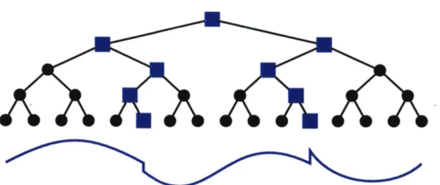
constraint, we now also require that our estimate obeys a graph connectivity constraint. For a given graph defined on our features, such a constraint enforces that the selected features form a connected component in the underlying graph. A concrete example of such a graph are protein-protein interaction networks in computational biology. From the biologist's point of view, graph-sparse solutions are more meaningful because they are more likely to correspond to a true biological process. But from the algorithmist's point of view, projecting onto the set of graph-sparse vectors is unfortunately an NP-hard problem.
Graph sparsity is not the only example of a constraint set that is hard to work with. Another example that has been intensively studied in the statistics literature is group sparsity, where the sparse solution consists of a few groups of variables [242]. Again, projecting on the set of group sparse vectors is NP-hard [33]. And even for sets with polynomial-time projections such as low-rank matrices or tree sparsity (also known as hierarchical sparsity), their
super-linear running time can be a bottleneck in practice. While these problems are not NP-hard,
improving the current running times of exact projections would still represent progress on fundament algorithmic problems. So how can we overcome this "projection bottleneck" in
PGD? Addressing this challenge is our second contribution in this context.
Tail approximations. When faced with a hard exact problem such as that in Equation 2.2, a standard approach in theoretical computer science is to study an approximate version of the problem instead. A natural way to relax the projection guarantee is as follows: for an input vector 0 r", we are now content with an approximate projection 0 E C satisfying
the guarantee
0- 2| < cT -min||Oin - 012, (2.3)
O'eC
where cr > 1 is the approximation ratio (for cT = 1, this is the same guarantee as an exact projection). In the following, we will refer to such a notion of projection as a tail
approximation.
Using an approximate projection of this form is a natural approach for speeding up PGD. Af-ter all, PGD is an iAf-terative algorithm where every step contributes only a small improvement to the solution quality. So insisting on an exact projection seems like an overly burdensome intermediate goal. But surprisingly, this intuition is false. As we show in Section 2.5, it is possible to prove that for any cT > 1, there are problem instances where PGD provably
fails. While this does not preclude the success of heuristics in practice, ideally we would like to understand whether it is possible to leverage approximation algorithms in a way that still provides strong performance guarantees.
Head approximations. We show that this is possible by utilizing a second,
complemen-tary notion of approximation: For an input vector Oin, our goal is now to find a unit vector
6 E C- Sd-I such that
( Qi,96) >
cw
-m ax
( Qif, I')(2.4)
O'ecnSd-1
where 0 < cW ; 1 is again the approximation ratio (and for cR = 1, this is also the same
guarantee as an exact projection). In this thesis, we refer to this notion of projection as a head
approximation. It is important to note that head and tail projections offer complementary
approximation guarantees. As soon as cR or cT are strictly bounded away from 1, a tail approximation cannot be converted to a high-quality head approximation (or vice versa).
By combining head an tail projections in the right way, we can prove that PGD with
approximate projections still converges to a statistically optimal solution in a broad range of estimation tasks (more specifically, under the same regularity conditions as in the previous subsection). Our approximation-tolerant extension of PGD is best illustrated in the well-conditioned regime (n 1 1), where we do not need the inner loop of the general algorithm. Denoting a tail approximation oracle with T and a head approximation oracle with 7, the main iterative step of PGD then becomes:
0i+1 <-
Tc(Ot
-
q -7(Vf (0))).
Compared to vanilla PGD, the main difference is that we now apply projections to both the gradient and the current iterate. Underlying this scheme is the insight that a tail approximation is only a useful guarantee when the input vector is already somewhat close to the constraint set. However, applying a full gradient update can lead us far outside the constraint set. To overcome this difficulty, we instead only take a head-projected gradient step. Clearly, this allows us to stay relatively close to the constraint set C. Moreover, we can show that the head-projected gradient step still makes enough progress in the function value so that the overall algorithm converges to a good soluton.
Instantiating our framework. While our approximation-tolerant version of PGD is an intriguing framework, at first it is not clear how useful the framework can be. To get an actual algorithm, we must instantiate the head and tail projection guarantees with concrete approximation algorithms for interesting constraint sets. Indeed, prior work on PGD with approximation projections could only instantiate their respective algorithms in restrictive settings [49, 82, 107, 108, 144, 145, 205]. To address this issue for our framework, we build a bridge between the continuous and discrete optimization worlds. By leveraging a wealth of results from the approximation algorithms literature, we construct new approximate projections for a broad range of constraint sets including tree sparsity, graph sparsity, group sparsity, and low-rank matrices (see Table 2.1). Even in cases where an exact projection is NP-hard (such as graph or group sparsity), our approximation algorithms run in nearly-linear time.
In all cases, our algorithms significantly improve over the running time of exact projections both in theory and in practice. While our theoretical analysis is not tight enough to preclude a moderate constant-factor increase in the sample complexity, the resulting estimators are still optimal in the O(.) sense. Experimentally, we also observe an interesting phenomenon: despite the use of approximate projections, the empirical sample complexity is essentially the same as for exact projections. Again, our results provide evidence that algorithmic problems become significantly easier in statistical settings. Moreover, they support the use
of approximate projections for optimization problems in statistics and machine learning.
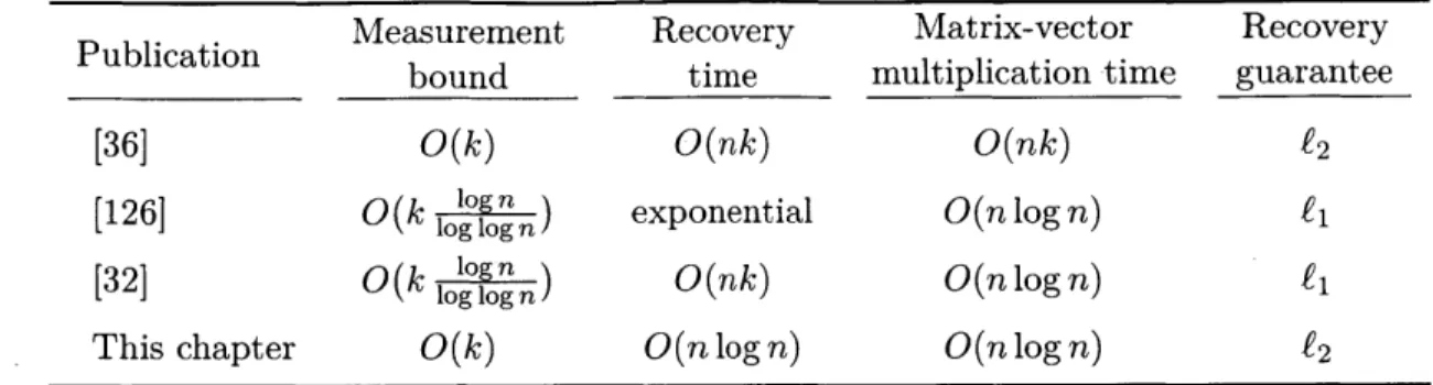
Best known time complexity Best known time complexity Constraint set of an exact projection of an approximate projection
(prior work) (this thesis)
Sparsity 0(d) Low-rank matrices 0(d'.5)
(r
d) Tree sparsity 0(d2 ) [64]O(d)
k-histograms 0(k2 - d2.5) 0(dl+E) EMD sparsity 0(d'.5 )Graph sparsity NP-hard [118] 0(d)
Group sparsity NP-hard [33] 6(d)
Table (2.1): The time complexity of exact and approximate projections for various constraint sets. In all cases beyond simple sparsity, approximate projections are significantly faster than the best known exact projections.
Further notes on the table: for simplicity, we use the 0 notation and omit logarithmic factors. The variable d denotes the size of the input (the dimension of the vector 0*). For matrix problems, the stated time complexites are for matrices with dimension xf'_ x V'ri so that the overall size (number of entries) is also d. The variable r denotes the rank of a matrix. For EMD sparsity, there is no known exact projection or hardness result. The
E
in the exponent of the running time for k-histograms is an arbitrary constant greater than 0.2.1.3 Outline of this part
In this chapter, we describe our core algorithms for optimizing over non-convex cones with approximate projections. Later chapters will then provide approximate projections for concrete constraint sets. The focus in this chapter is on our new two-phase version of projected gradient descent since it is the most general algorithm. We will also provide more specialized versions for the RIP setting (K ~ 1) since we use them in later chapters.


![Figure (5-2): Compressive sensing recovery of a ID signal using various algorithms (signal parameters: n = 1024, k = [0.04n] = 41, m = [3.5k] = 144)](https://thumb-eu.123doks.com/thumbv2/123doknet/13923073.449926/142.917.137.736.101.639/figure-compressive-sensing-recovery-signal-various-algorithms-parameters.webp)
