HAL Id: insu-01512563
https://hal-insu.archives-ouvertes.fr/insu-01512563
Submitted on 24 Apr 2017HAL is a multi-disciplinary open access archive for the deposit and dissemination of sci-entific research documents, whether they are pub-lished or not. The documents may come from teaching and research institutions in France or abroad, or from public or private research centers.
L’archive ouverte pluridisciplinaire HAL, est destinée au dépôt et à la diffusion de documents scientifiques de niveau recherche, publiés ou non, émanant des établissements d’enseignement et de recherche français ou étrangers, des laboratoires publics ou privés.
Uncertainty assessment of volumes of investigation to
enhance the vertical resolution of well-logs
Pedram Masoudi, Tahar Aïfa, Hossein Memarian, Behzad Tokhmechi
To cite this version:
Pedram Masoudi, Tahar Aïfa, Hossein Memarian, Behzad Tokhmechi. Uncertainty assessment of volumes of investigation to enhance the vertical resolution of well-logs. Journal of Petroleum Science and Engineering, Elsevier, 2017, 154, pp.252-276. �10.1016/j.petrol.2017.04.026�. �insu-01512563�
Author’s Accepted Manuscript
Uncertainty assessment of volumes of investigation
to enhance the vertical resolution of well-logs
Pedram Masoudi, Tahar Aïfa, Hossein Memarian,
Behzad Tokhmechi
PII:
S0920-4105(16)31301-8
DOI:
http://dx.doi.org/10.1016/j.petrol.2017.04.026
Reference:
PETROL3966
To appear in:
Journal of Petroleum Science and Engineering
Received date: 14 December 2016
Revised date:
13 April 2017
Accepted date: 19 April 2017
Cite this article as: Pedram Masoudi, Tahar Aïfa, Hossein Memarian and Behzad
Tokhmechi, Uncertainty assessment of volumes of investigation to enhance the
vertical resolution of well-logs,
Journal of Petroleum Science and Engineering,
http://dx.doi.org/10.1016/j.petrol.2017.04.026
This is a PDF file of an unedited manuscript that has been accepted for
publication. As a service to our customers we are providing this early version of
the manuscript. The manuscript will undergo copyediting, typesetting, and
review of the resulting galley proof before it is published in its final citable form.
Please note that during the production process errors may be discovered which
could affect the content, and all legal disclaimers that apply to the journal pertain.
1
Uncertainty assessment of volumes of investigation to enhance the
vertical resolution of well-logs
Pedram Masoudi
1, Tahar Aïfa
1,*, Hossein Memarian
2, Behzad Tokhmechi
31
Géosciences-Rennes, CNRS UMR6118, Université de Rennes 1, Bat.15, Campus de Beaulieu, 35042 Rennes cedex, France
2
School of Mining Eng., College of Eng., University of Tehran, North Kargar, 1431954378 Tehran, Iran
3
Department of Petroleum Engineering, University of North Dakota, 243 Centennial Drive Stop 8154, Grand Forks, ND 58202-8154, USA
*
Corresponding author: tahar.aifa@univ-rennes1.fr Abstract
Whereas well-log data are dense recordings, i.e. low sampling rate, there is a high depth uncertainty. The depth uncertainty originates from the volumetric nature of well-logging that each record belongs to a volume of investigation, around the logging tool. The developed algorithm in this work consists of two parts: (i) uncertainty assessment using Dempster-Shafer Theory (DST). The lower (upper) uncertainty boundary of each well-log is calculated by belief (plausibility) function. (ii) Four simulators are designed for scanning the uncertainty range in order to enhance the vertical resolution of well-logs (~60 cm) by generating simulated-logs (vertical resolution of ~15 cm). Shoulder-bed effect is reduced simultaneously with resolution improvement, resulting in more accurate thin-bed characterization. In order to validate functionality of the simulators, two error criteria are considered: ideal- and constraint-based errors. Ideal-based error is applicable in synthetic-logs where the rock specifications are completely known through ideal-synthetic-logs. However, constraint-based error does not need ideal-log. It measures the error due to the volumetric nature of the well-logs, hence applicable in the real cases. The high correlation (R2=0.89) between both the errors indicates that the second criterion is precise for validation. Step-by-step procedure of the algorithm is shown in detail on synthetic and real data (a cored interval). Finally, DST-based algorithm is not only automated but also more accurate than geometry-based thin-bed characterization method. The error bars of characterizing gamma, density and neutron porosity of thin-beds are lower in DST-based algorithm by 100%, 71% and 66%, respectively.
2
Abbreviations
Bel, belief function; BOE, body of evidence; dist, distance; DST, Dempster-Shafer theory; DT, sonic log (slowness log); FE, focal element; FEr, focal element of recording; FEt, focal element of target; fr, fraction; GIS, geographic information system; GR, gamma ray log; id, ideal; int, interpolation; m, mass function; MSE, mean square error; NPHI, neutron porosity log; PDF, probability distribution function; Pls, plausibility function; pv, petrophysical value; rec, recording; RHOB, bulk density log; RMSE, root mean square error; sim, simulation; SE, shoulder-bed effect; SR, sampling rate; std, standard deviation; UNC, uncertainty; VR, vertical resolution; wl, well-log
Keywords: shoulder-bed effect, volumetric measurement, vertical resolution, thin-bed, depth uncertainty, realization prioritizing
1. Introduction
Vertical resolution of logging tools is reported from some centimetres, e.g. Micro Spherically Focused Log (MSFL), to about 100 cm, e.g. Spontaneous Potential (SP). So characterizing geological beds thinner than the vertical resolution is imprecise even if the sampling rate is precise enough (McCall et al., 1987; Passey et al., 2006; Masoudi et al., 2017). Acquired petrophysical data belong to a three dimensional space namely volume of investigation. Projection of this 3D volume on the 1D well axis is called vertical resolution.
Geological and technical aspects of well-logging were overwhelmed in the first publications concerning resolution enhancement. Only signal-processing theories, Weiner and Kalman filter, were developed for the purpose of increasing frequency of the well-logs (Foster et al., 1962; Bayless and Brigham, 1970). The other practical issue of signal processing algorithms is lack of knowledge about the theoretical parameters since there was no confidence about the used parameters (Lyle and Williams, 1987).
Until 1987, the studies were totally theoretical, however practical improvement of vertical resolution of well-logs was basically done within the years 1989-1990, when industrial researchers of
3
Schlumberger, Halliburton and British Petroleum played part. They used geometrical and numerical analysis for developing easy-to-apply procedures to improve well-log resolution.
The beds thinner than 2 feet (60.96 cm) cannot be properly evaluated by (far) density log. Based on geometrical reasoning, a wise correction to enhance density log for characterizing thin-beds (less than 6 inches or 15.24 cm) is developed. The main idea was inferring the high-frequencies from short-interval density measurements (applying a low-cut filter), and adding the remained high-frequencies to the long-interval density measurements (Flaum et al., 1989). Inspired from the former work, resolution of compensated neutron log is enhanced too (Galford et al., 1989). In addition, the contact of two layers with different porosities is identified with less uncertainty: ±2 inches (5.08 cm) rather than ±6 inches (15.24 cm) (Gartner, 1989). In another similar work, it is assumed that the attenuation log of Electromagnetic Propagation Tool (EPT) and clay volume (derived from geochemical logging) are strongly correlated linearly. Hence, high-frequencies are inferred from high-resolution EPT log, and coherent small changes for geochemical logs are re-created (Flaum, 1990).
True understanding of mechanism and spatial response of well-logs is important in a successful well-log interpretation. This necessity becomes more rigorous in heterogeneous media. Monte Carlo simulation is used to study spatial response (mostly horizontal resolution) of density log. It is found that in carbonate formations, 75% of density log response captures the first 8 cm from the borehole wall and 90% captures till 12 cm (Petler, 1990).
Based on the previously developed logical equation for vertical resolution correction (Flaum et al., 1989), a sensitivity analysis is addressed in a three dimensional space, using Monte Carlo simulation. Using density and neutron logs in high-angle (near horizontal) wells, the uncertainty of identifying depth of bed boundaries is about ±2.5 inches (6.35 cm). This uncertainty rises under shoulder-bed effect to about ±10 inches (25.4 cm) and ±15 inches (38.1 cm) by density and neutron logs, respectively.
Shoulder-bed effect is attenuation of a thin-bed trace on a well-log, when the thin-bed is sandwiched between two thicker beds (RP, 2007; Torres-Verdín et al., 2009; Sanchez Ramirez et al.,
4
2010). This uncertainty in highly deviated wells is justifiable by the fact that neutron and density tools are designed and calibrated for vertical wells; so, standard interpretations are incorrect (Mendoza et al., 2006).
Within the domain of subjective probability, Dempster-Shafer Theory (DST) is introduced as a generalization of Bayesian theory that provides upper and lower probability values, namely plausibility and belief functions, respectively (Dempster, 1967, 1968). Mathematical basis of this theory is redeveloped and well-explained (Shafer, 1976, 1990), so became well-known as the evidence theory of Dempster-Shafer.
Application of DST in geosciences is mostly developed in Geographic Information System (GIS) (Feizizadeh et al., 2014; Saeidi et al., 2014; Neshat and Pradhan, 2015), whereas it is very limited in the petroleum geology. The first DST application in the petroleum industry was published in 1994 (Aminzadeh, 1994), meanwhile the next articles were published ten years after (Masoudi et al., 2014; Arab-Amiri et al., 2015a,b). In the mentioned articles, the DST was used at the level of decision fusion (using Dempster rule of combination), while in the current article, an application of DST is developed for pre-processing well-logs (using the basic concepts of evidence theory).
The essential publication in resolution enhancement, conducted by Flaum et al. (1989), requires (i) dual spacing measurements, i.e. one transmitter and two receivers and (ii) correlation assumption between dual spacing logs or sometimes between different well-logs. Here, an uncertainty-based methodology is developed to provide a mapping from the domain of vertical resolution of recordings (well-logs) to vertical resolution of target, which is 4 to 6 times more precise. The methodology is based on DST, and integrates multi-evidences for new inferences regarding resolution enhancement (Dempster, 1967, 1968; Shafer, 1976, 1990).
Application of DST-based algorithm is checked on synthetic and real datasets. Synthetic dataset is important to check and validate the algorithm under controlled situations. Ideal-based error is a reference for validating constraint-based error and DST-based algorithm by means of synthetic data. Constraint-based error is designed to measure the error of the algorithm in real (non-ideal) well-logs. It
5
is also used as a criterion for prioritizing and selecting the best realization, i.e. output of the simulation process, in the real dataset.
2. Datasets
2.1 Basic definitions
In this article, there are four key terms to introduce the datasets. “Well-log” and “real-log” are used to describe real data. In the synthetic data, “synthetic-log” and “ideal-log” are used. Synthetic-log is equivalent to well-log, and ideal-log is equivalent to real-log.
Well-log records intrinsic or induced properties of the rocks and their fluids (Gluyas and Swarbrick, 2009). Such records, acquired through a well, are either one dimensional, like gamma ray log, or two dimensional as image logs. Well-log is also known as borehole log since data are captured through the wellbore.
Real-log reflects real properties of the well-bore. Well-logs are imprecise (apparent) in reflecting real properties, especially in thin-bed conditions because well-logs are convolved data (Gartner, 1989). The convolution is done over the vertical resolution of the logging tool. When the vertical resolution approaches zero, the well-log converges the real-log.
Ideal-log is equivalent to “real-log” in synthetic datasets. It is defined by the user, while real-log represents rock nature. Finding real-log is an open problem in the well-logging, while ideal-log is definite. So, useful in validation.
Synthetic-log is convolution of ideal-log over a vertical resolution. It resembles well-log in real data.
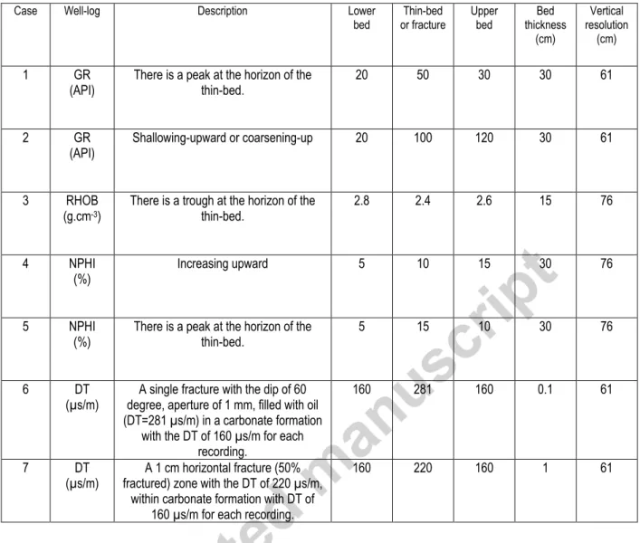
2.2 Synthetic cases
The first stage in generating a synthetic-log is defining specifications of its ideal-log (Table 1). Vertical resolution is zero in ideal-logs, i.e. no depth uncertainty.
In Table 1, each case represents a petrophysical change in presence of a thin-bed (cases 1-5 and 7) or a single fracture (case 6). Synthetic-log generator for thin-beds (cases 1-5 and 7) convolves the
6
ideal-log (Masoudi et al., 2017). For the case 6, simulator generates a synthetic-log based on geological specifications of a single fracture. It calculates the effect of a predetermined fracture on the well-log (Mazaheri et al., 2015).
2.3 Real data
Well-log data (GR, RHOB, NPHI and DT) of five exploratory wells are used to check the developed methodology. The wells are located on the axis of an anticlinal oil-field in the Abadan Plain, SW Iran (Figure 1a). The well-logs are limited to the interval of Sarvak Formation (Figure 1b), a homoclinical carbonate ramp, deposited from Albian to Turonian (Ghazban, 2009). In homoclinical carbonate ramps, there is a slight seabed dip toward the sea. This term belongs to a topological classification of carbonate ramps (Read, 1985). Vertical resolution of well-logs (Table 2) within Sarvak interval is previously inferred from geostatistical variography (Masoudi et al., 2017).
2.3.1 Volumetric constraint of well-logs
Although a well-log value is a recording over a volume of investigation, it is assigned to a single depth (Figure 2a). In fact, small-dimension heterogeneities, i.e. variations smaller than the volume of investigation, are ignored by the logs. In mathematical language, the recorded value is the integral of petrophysical values over geological beds (Equation 1). The equivalent discrete form (Equation 2) is presented on Figure 2b.
Note that the depth of investigation is out of the scope of this paper, and it is only sketched (Figure 2) to illustrate the mechanism of logging. The focus of the figure and the article is on the vertical resolution. The recorded well-log (black circles) with the vertical resolution of , is replaced by simulated-log (white circles) with the vertical resolution of . The superscripts r and t stand for recording and target, respectively.
( ) ∫ ( ) ( )
7
( ) ∑ ( ) ( )
⌊ ⌋
⌊ ⌋
(2)
where ( ) is the well-log value at depth , ( ) is real petrophysical value of the formation at depth . scans a focal element of recording (vertical resolution) around the depth . Simulated-log, ( ), is discrete equivalent of ( ). The weight, ( ), is for increasing the relative impact of petrophysical values, closer to the centre of volume of investigation. stands for focal element of recording, and is equivalent to the vertical resolution of tool. stands for sampling rate, distance between two adjacent records.
In the Equations 1 and 2, ( ) is a known measured value, and are known specifications of logging tool. The weight ( ) is a linear function of depth. So, the only unknown function is ( ) or ( ), could be determined by a back propagation procedure. The concept of “volumetric constraint of well-logs” is an important technical fact that is used here not only in an optimization process but also for validation and choosing the best realization.
3. Dempster-Shafer theory
DST enables a mathematical tool for inferring and decision-making in uncertain situations. The most basic difference between the Bayesian theory of probability and DST is that neither Probability Distribution Function (PDF) nor membership function are needed in DST. The first stage in applying DST is defining a Body Of Evidence (BOE) that is a basic structure for calculations. BOE consists of two parts: (i) focal elements: some subsets, containing possible happenings; (ii) mass function: a measure for the happenings, which is equivalent to the probability function. Each mass value is assigned to a focal element, and can move freely inside it, while satisfying imposed limitations of the problem. The displacing of mass values creates belief (plausibility) function which is the minimum (maximum) possible mass in a focal element. As an example, mass of focal element “A” can move freely within it (Figure 3a); while probability of “A” is fixed according to a predefined triangular PDF (Figure 3b).
8
3.1 Body of Evidences
3.1.1 Focal elements
In a series of observations (or measurements, evaluations, etc.), each evidence is assigned to a subset, called focal element. As this name suggests, the available evidence focuses on focal elements (Klir and Yuan, 1995). Here, focal elements are defined as depth intervals, i.e. focal elements are one dimensional. We have defined two types of focal elements: (i) recording (r) that represents vertical resolution of the logging tool, and (ii) target (t) which is the target resolution, defined by user. Figure 4 shows focal elements of recording and target when vertical resolution is four times larger than sampling rate. In fact, the aim is to improve the vertical resolution of well-logs from the focal element of recording ( ) to a focal element of target ( ).
3.1.2 Mass function of focal element of recording
Corresponding to each , a mass value is defined, which is free to move inside it. In addition to the BOE, redistribution of the mass has to obey the constraints of the problem, here geological and technical conditions. Mass function is always non-negative, and the summation of mass values over all the focal elements should be one (Equation 3) (Liu and Yager, 2008). The symbol “ ” means that the equation is defined by user, and it is not derived from calculations.
∑ ( )
(3)
Petrophysical well-logging is a volumetric measurement, i.e. assigns a recorded value to a volume of investigation. So, these recordings satisfy the requirements for designing a BOE: log values as mass functions, corresponding to the volume of investigation (focal elements). Hence, uncertainty of well-logs could be modelled by DST, and the ignored geological heterogeneity could be rebuilt. In order to satisfy Equation 3, for each log, mass function is defined as normalized value of well-log. Modelling unpredictable situations is not the concern of this study, therefore the mass function of null set ( )
does not take part in the calculations, i.e. ( ) . The null function in DST corresponds to a situation that the defined BOE is not valid; e.g. well-logging under abnormal situations: high-noise, logging tool does not work properly, turbulences, etc.
9
3.1.3 Theoretical belief and plausibility functions for focal elements of target
As illustrated in Figure 4, the recorded well-log is acquired over four subset focal elements of target. The petrophysical value of each focal element of target affects the four adjacent well-log recordings. In the language of BOE, mass values of the four adjacent focal elements of recording could freely pass through a common focal element of target ( in Figure 4). DST-based structure helps us to find lower (belief) and upper (plausibility) probabilities for each focal element of target (Equations 4 and 5). Belief (plausibility) function shows the least necessary (most possible) mass value within the focal element of target (Liu and Yager, 2008).
( ) ∑ ( )
(4)
( ) ∑ ( )
(5)
3.2 Compatibility of DST with well-logging
3.2.1 Main uncertainty assessment theories
There are three major theories for decision-making in uncertain situations: Bayesian theory of conditional probability (Bayes and Price, 1763), DST and possibility theory of fuzzy logic (Zadeh, 1999). Comparative studies could be done theoretically and fundamentally (Klir and Yuan, 1995; Zadeh, 1999), or based on application check and outcomes (Challa and Koks, 2004; Tangestani, 2009). In the next part, applicability of probability and possibility theories is shown through two examples. Then, for the case of volumes of investigation of well-logs, the importance of DST, and its inconsistency with the other two theories is discussed.
3.2.2 Domains of uncertainty theories
The analysis of a dice game, using probability theory, leads to a PDF with the probability of for each of the six sides. In this example, the BOE consists of six focal elements, each containing only one number (one to six). The focal elements do not have any intersection with each other, e.g. when the dice shows number four, it cannot hold any other value simultaneously. So, the theory of probability is compatible with dice game.
10
In the other example, consider a person who may eat some eggs (e.g. one to six eggs) at breakfast. Probability theory could be used to predict how many eggs he eats every day. So, due to statistics (a
priori knowledge), he mostly eats two or three eggs per day, rarely zero, one or four, and never five or
six eggs. Thus, the result is a PDF with a value of zero for five and six eggs, and a height at two and three eggs.
Approaching this problem by the possibility theory means that possibility of eating four eggs has the possibility of eating three, two or one egg(s). In the language of the set theory, in each pair of subsets, one is subset of the other. So, the focal elements are eccentric and the result will be cumulative (a property of the fuzzy measure) with the highest possibility for eating one egg, and the lowest possibility for eating five eggs.
Volume of investigation does not have probabilistic nature, so PDF, i.e. the theory of probability, is not an ideal theory for modelling them. Instead, volume of investigation has a membership nature, because it shows belongness of a volume to a record. So, fuzzy membership function, i.e. the theory of possibility, or focal element, i.e. DST, could be used.
3.2.3 Consistency and configuration of focal elements in uncertainty theories
It is shown by the examples that the probability (possibility) theory is applicable in separated (eccentric) focal elements. In the DST, the property of freely movement of the mass function within focal elements has made it powerful in assessing all BOEs (separated, eccentric, etc.). So, wherever possibility and probability theories work, DST works too (Table 3).
When the theories of probability (possibility) and DST are both valid, it is called that they are consistent. Probability and possibility theories are never consistent with each other, because they are two end-members of configuration of focal elements. To verify the consistency, either focal elements or consistency conditions should be checked. The simplest consistency condition (Relation 6) is the probability value between the belief and plausibility values (Klir and Yuan, 1995):
11
Defined (Figure 4) are comparable with the bottom-most case in Table 3: the focal elements are neither separated nor eccentric, but they have intersected intervals. So, analytically, neither probability nor possibility theories are expected to be helpful in assessing uncertainty of the well-logs. The theory of probability does not provide any reasoning for the intersecting focal elements like in well-logging. On the other hand, Relation 6 is not always valid, i.e. the output of the probability measure (averaging function) is not always between belief and plausibility values (Figure 5). The incompatibility is due to BOE of well-logs and the axiomatic structure. The conclusion of this part is to emphasize on the compatibility of DST with the focal elements in volumetric well-log data though DST is not still well-developed in well-log interpretations.
4. The proposed methodology
4.1 Part one: DST-based uncertainty range
4.1.1 Geological constraints as an axiomatic structure
Whereas Equations 4 and 5 are valuable theoretically for defining belief and plausibility, they are not practical because the uncertainty range will be too large due to: (i) belief function that is absolutely zero since the condition of Equation 5 is never valid in the defined BOE; (ii) plausibility
which is always a too big value, i.e. summation of adjacent recordings.
An axiomatic structure is then designed to impose geological facts and DST-based constraints on belief and plausibility functions. Applying three axioms results in a reasonable uncertainty range: (i) volumetric constraint of the well-logs: for each horizon, belief (plausibility) is the minimum (maximum) well-log value within the interval of a vertical resolution, centred at the depth of recording. It should be taken into account that we cannot generate or remove the mass, but the mass can move within its corresponding focal element of recording. (ii) No uncertainty in homogenous conditions: if the well-log remains constant within an interval of at least one vertical resolution, i.e. a focal element of record, there would be no uncertainty range in the middle of the horizon. Thus belief, plausibility and mass functions will be equal. (iii) Shoulder-bed effect: at peaks and troughs a destructive effect occurs which have to be compensated. So, at peaks (troughs), belief (plausibility) has to be equal to the mass function (Figure 5).
12
4.1.2 Practical functions of belief and plausibility
Based on the axiomatic structure and defined mass function on the , belief and plausibility for is formulated (Relations 7 and 8):
( ) { ( ) ( ) ( ) ( ) ( ) ( ) ( ) ( ) ( ) ( ) ( ) ( ) ( ) ( ) ( ) ( ) ( ) (7) ( ) { ( ) ( ) ( ) ( ) ( ) ( ) ( ) ( ) ( ) ( ) ( ) ( ) ( ) ( ) ( ) ( ) ( ) (8)
If ( ) is neither at peak nor at trough, then the minimum (maximum) of mass functions of intersecting is defined as the belief (plausibility) value. If ( ) is at the peak (trough), the belief (plausibility) is defined to be the exact amount of the well-log, and the plausibility (belief) will be the maximum (minimum) of intersecting plus (minus) an epsilon. The epsilon is a positive value to compensate the shoulder-bed effect, and will be optimized in the next section (Figure 5). Finally, both belief and plausibility values are rescaled to well-log range. From the application viewpoint, normalization (Equation 3) and rescaling could be ignored, since here the goal is not multi-sensory fusion.
4.1.3 Compensating shoulder-bed effect by the epsilon
For compensating shoulder-bed effect, the epsilon ( ) is defined by comparing the well-log to its weighted averaging filter. A well-log itself is a weighted averaging operator over petrophysical properties of a volume of investigation. So, we applied the same smoothing on the well-log. Then, the difference between the original well-log and its smoothed curve is considered as to compensate the shoulder-bed effect at peaks and troughs (Figure 5). In the validation part, it is shown that cannot fully compensate the shoulder effect, since the well-log is much smoothed, and a multiplier, named factor of Shoulder-bed Effect (SE) is necessary for calibration. The concept of is comparable with resolution enhancement equation of Flaum et al. (1989).
13
4.2 Part two: Simulators
Since well-log is a volumetric data acquisition, a recording is not exactly the same value as the real petrophysical value of the measuring point. The uncertainty range helps us to have a range interval in which the real petrophysical value (real-log) probably occurs. In this part, four DST-based simulators are developed in order to enhance the vertical resolution of the original well-log. In fact, simulated-logs are corrected well-simulated-logs due to the vertical resolution.
4.2.1 Random simulator
This is the simplest designed simulator that only produces uniform random values between belief and plausibility. Heterogeneity is the highest in the uniform distribution, so the simulator can generate the most heterogeneous realizations, which is usually desired in unknown geological conditions. In fact, this is a base simulator, and it is expected that other simulators provide more accurate results in general.
4.2.2 Random-optimization simulator
Second simulator starts by random simulation. But a sequential optimization is going to be applied on the generated random values, iteratively. The optimization is based on the volumetric constraint of well-logs. It means that each record should be a weighted average of simulated values within an interval of a vertical resolution (Equation 9 and Figure 6). Within the interval, distance is defined as extraction of well-log from weighted average of the corresponding simulations (Equation 10 and Figure 6). ( ) ∑ * ( ) ( ⌊ ⌋ )+ ⌊ ⌋ ⌊ ⌋ (9) ( ) | ( ) ( )| (10)
where ( ) is weighted average of simulated-log, ( ), over a vertical resolution. Vertical resolutions of ( ) and ( ) correspond to and , respectively. ( ) is distance of the
14
( ) and ( ) are functions of depth. is number of adjacent simulations, within a vertical resolution, e.g. in Figure 6.
Note that the methodology could be applied to all the possible combinations of sampling rate and vertical resolution if an appropriate is found. is a linear weight for prioritizing closer
simulations to recording depth. To calculate the weights, the natural values 1, 2, 3, etc. are primarily attributed to the parameter , in function of distance. Then, the weights are normalized by the summation of .
After a random generation, the corresponding distance of the first simulations is calculated
(Equation 10). For simplicity, and to avoid re-modification of the former optimized points, the distance is compensated only by one simulation point, which is the closest to the well-log record, e.g. S3 in Figure 6. The optimization continues through the well till the end of the well-log. After each round of simulation, summation of new distances is stored as the error of modified simulated-log. Modification could be iterated up to convergence of error plot. The convergence cut-off is a stop condition of the optimization process. It is recommended to set the convergence cut-off of 0.001 for the summation of all distances. The stages of the optimization algorithm are introduced in the section “4.4 The algorithm/ v.b”.
4.2.3 Recursive simulator
This simulator consists of two stages. In the first stage, uniform random values between belief and plausibility will be generated for the first ( ) data. In the second stage, the simulated-log for
the remaining depths will be calculated recursively. The recursive Equation 11 is derived from the volumetric constraint of well-logs (Equation 9).
( ⌊ ⌋) ( ⌊ ⌋) ∑ * ( ) ( ) ( ⌊ ⌋ )+ ⌊ ⌋ ⌊ ⌋ (11)
15
4.2.4 Recursive-optimization simulator
The final simulator consists of three stages. The two first stages of recursive simulator, followed by the optimization process of random-optimization simulator. The interrelations and brief of the stages of the four developed simulators are provided in Figure 7a. Two of the simulators (random and random-optimization) start with free random generation, and two others (recursive and recursive-optimization) start with constraint-based random generation.
4.3 Validation criteria
Different realizations could be generated by the introduced simulators. It is necessary to have a measure to validate and prioritize realizations, and finally choose the most accurate realization. An ideal criterion is to compare the simulated-log with the ideal-log (Equation 12).
∑| ( ) ( )|
(12)
where ( ) and ( ) are ideal- and simulated-log, respectively. The subscript of “int”
shows that the simulated-log is interpolated at the depths of the ideal-log. Both are functions of depth but due to depth mismatch (sometimes) between simulated- and ideal-log, the simulations have to be interpolated to the exact depths of the ideal-log. stands for total ideal-based error.
Evidently in subsurface geology, we do not have ideal-logs, so Equation 12 is practical only in synthetic cases. In real data, instead of ideal error, summation of distances (Equation 10) is used as a validation criterion. Since the distance is based on the volumetric constraint of well-logs, the criterion is named “constraint-based error”. Both ideal- and constraint-based errors are applied to synthetic data and it is shown that they are highly correlated (R2=0.89, Figure 11). The advantages of constraint-based error are: (i) providing error for each horizon (error profile), (ii) calculating total error (integral of error profile), (iii) validation only by the well-log, and no need to use other measurements like core, well-tests or ideal-log, and (iv) highly correlated with ideal-based error.
4.4 The algorithm
The algorithm consists of two parts: (i) DST uncertainty assessment and (ii) simulation (dashed rectangles, Figure 7b). In the first part, the uncertainty range of each record is defined and in the
16
second part, simulation is done within the uncertainty range. The details of stages of algorithm are provided below, and the background of each part is previously discussed.
i. Input: the algorithm assesses well-logs individually, so one well-log has to be selected to apply the algorithm to it. The well-logs without volume of investigation, like geochemical logs or calliper log, could not be chosen. Both synthetic-log and well-logs could be used for this algorithm.
ii. Vertical resolution: corresponding to the vertical dimension of volume of investigation of the chosen well-log, the vertical resolution should be defined. The catalogue of the logging instrument could be used for this purpose. In case no catalogue is available, vertical resolution could be approximated by a measure of continuity. To find out the number of adjacent records correlated with each other, three steps are addressed: (a) experimental variography analysis, (b) selection of its linear part, and (c) considering vertical resolution as its length.
iii. Mass function: spatial domain of each well-log record is considered as a linear focal element, called focal element of recording ( ). The recorded well-log value is considered as the mass value within its corresponding . Theoretically, the mass value has to be normalized in order to satisfy Equation 3. However, since in this algorithm there is no multi-sensory fusion, the normalization is not necessary. The and its mass function construct a BOE, which should be honoured in the next step.
iv. Belief and plausibility functions: goal of DST part of the algorithm is to provide an evidence-based reasoning for intersection of the adjacent . Based on ratio of vertical resolution to sampling rate, number of adjacent intersecting records (Figure 4) is calculated. The intersecting interval is called focal element of target ( ). The mass functions, which move within different , provides a range of mass values for . Mass value of cannot exceed maximum mass value of intersecting (Figure 4). Therefore, for honouring the records (which are our evidences) the belief (plausibility) is limited to the minimum (maximum) of intersecting mass functions (Relations 7 and 8). Belief and plausibility functions are limits of the created uncertainty range. This process contains two steps: (a) ⌊
⌋, and (b) calculating belief and plausibility
17
v. Simulation: simulation could be done by one of four designed simulators (Figure 7a).The simulator could be chosen according to a validation criterion (Equation 10 or 12). All the simulators start by a random generation stage. In recursive simulator, random generation is limited to a few number of focal elements. However, in random simulator, all the elements are guessed randomly. If the designed optimization process is applied to the outputs of random or recursive simulators, the errors will converge.
(a) If recursive simulator is used, Equation 11 will be used for calculating simulated-log for the rest of the depths.
(b) If the optimization process is used:
(b1) The distance (Equation 10) is computed for the ith well-log data.
(b2) The distance is compensated by the ith simulated-log data.
(b3) i=i+1, then go to the line (b).
vi. Validation: the validation is done either regarding ideal-log (ideal-based error, Equation 12) or well-log (constraint-based error, summation of Equation 10). Ideal-based error is only applicable in synthetic cases, and constraint-based error could be calculated for both synthetic and real data. In a homogenous formation, the order of the errors is like in Figure 8. This general order could be violated in heterogeneous formations. So, precision of all the simulators have to be always checked to find the most accurate simulated-log.
vii. Simulated-log: the simulated-log with the least error is selected as an alternative for the original well-log. The advantage of the simulated-log is that its vertical resolution is equal to the which is much more accurate than the original well-log resolution.
5. Application check on synthetic cases
Worthy to remind that the aim of the developed methodology is to get closer to a real-log (or an ideal-log), corresponding to the well-log (or the synthetic-log). Four simulated-logs can be generated by the designed simulators. All the simulators are applied on all the cases (Table 1). The predefined ideal-log (stars) and corresponding synthetic-log (black dots) of case 1 are presented in Figure 8a, and
18
the other cases are interpreted in the Appendix A. To calculate ideal-based error, the realizations are first interpolated to the depths of the predefined ideal-log (if necessary). Then, the mismatch of the realization with the ideal-log is calculated for each depth, called error profile (Figure 8b). As indicated in Figure 8c, the summation of the error profile through the well-log is named total ideal-error.
Random simulator never satisfies the goal. In this case, it has neither recreated the shape of the ideal-log, nor its real value. Comparing to other simulators, it has the highest profile and total errors (Figure 8c). The best realization of random-optimization simulator is exactly the realization of recursive-optimization simulator. Both random-optimization and recursive-optimization simulators provided the same result for 48 iterations out of 50. They pass through the same optimization procedure (Figure 9), so convergence of the realizations is justifiable. The same reasoning is valid for the other cases (Appendix A).
5.1 Discussion on results of the synthetic cases
Since none of the simulators were able in detecting the single fracture of case 6, it is exempted from further evaluation. Both ideal- and constraint-based errors agree that recursive-optimization simulator is the most accurate in cases 1, 3 and 5 (Table 4). In case 2, random-optimization simulator is the best. However recursive-optimization simulator is a competing simulator, and it is only 0.6% less accurate than random-optimization simulator. The same for case 7. For case 4, constraint-based error votes for recursive-optimization simulator though ideal-based error selects random simulator. The descriptions are summarized in Figure 10. From the viewpoint of ideal-based error, in 50% (8%+42%) of the cases, recursive-optimization simulator provides the best output (Figure 10). Random-optimization simulator is the most accurate simulator only in 33% (8%+25%) of the cases. On the other hand, from the standpoint of constraint-based error, recursive-optimization simulator is also the best, since it is valid in 67% (8%+42%+17%) of the cases.
There is another advantage for recursive-optimization simulator: optimization starts from a lower error value, compared to random-optimization simulator, subsequently, convergence is reached within only 6 epochs (Figure 9). Therefore, less time is required for recursive-optimization simulator to reach a local minimum point. In the synthetic cases, recursive-optimization simulator is the best. Recursive
19
simulator was never successful, compared to the others; but random simulator provides the best result only in case 4 whereas the other simulators are not satisfactory (Table 4 and Figure 10).
5.2 Validating constraint-based error by the synthetic cases
It is impossible to calculate ideal-based error in the well-logs, because it needs an ideal-log that does not exist in the real data. Instead, it is suggested to use developed constraint-based error; i.e. summation of distances in Equation 10. To verify constraint-based error, the synthetic data are used. The 24 pairs of errors (Table 4) are plotted (Figure 11). Cross plot of errors shows high positive correlation between the two errors (R2=0.89), however constraint-based error is an overestimation of ideal-based error. Therefore, the behaviours of both the errors are similar, and constraint-based error could be used as a validation criterion in real datasets.
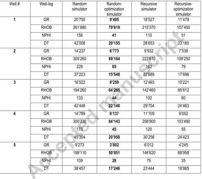
6. Application to the real data
The four developed simulators are applied on the four well-logs of the five wells under study. Due to total constraint-based error, random-optimization simulator is the most accurate simulator in all the situations (Table 5). However, the error of recursive-optimization simulator is not much higher than that of random-optimization simulator. This may be interpreted such as random-optimization simulator searches for the minimum points more effectively, hence it can get closer to the global optimum point but recursive-optimization method does not check the variety of possibilities for each depth. Further studies are applied on random-optimization simulator.
6.1 Optimizing factor of Shoulder-bed effect
The factor of Shoulder-bed Effect (SE) is the only parameter in the simulators that requires manual optimization. SE is checked from 2 to 7 for random-optimization simulator (Table 6). The optimum SE for GR and DT is 3, but for GR in the second well the optimum SE is 4. For RHOB and NPHI, the optimum SE is between 5 and 7.
6.2 Results of resolution improvement of well-logs
To apply random-optimization simulator to well-logs, the optimized parameters (Table 7) are used. Here, the results of resolution improvement are illustrated for the interval of 3157-3159 m, well#1 (Figure 12a). Each track in Figure 12 contains: (i) the original well-log (solid black line) with the
20
vertical resolution of 61-91 cm (Table 2); (ii) the uncertainty range (blue zone) which is between the belief and plausibility; (iii) ten realizations from random-optimization simulator (dots), and (iv) the best one is marked by dashed line (simulated-log). The vertical resolution of the realizations is 15 cm ( in Figure 2b).
The uncertainty range honours the predefined axiomatic structure (Relations 7 and 8). (i) The lower (upper) boundary is the minimum (maximum) value over the neighbouring values. (ii) The
uncertainty in the top half metre (3157-3157.5 m) is about zero due to constant value of the original well-log for some neighbouring records. (iii) The SE is compensated (to some degree) by the sparks at the peaks and troughs; i.e. small variations are amplified (Figure 12a).
All the well-logs show less uncertainty range in the half top metre (3157-3157.5 m, Figure 12a), compared to the other parts. It means that the top part is more homogeneous, while the heterogeneity arises downward. Therefore, any interpretation (estimation of porosity, permeability, etc.) within the homogeneous part is more certain than the heterogeneous part. In fact, heterogeneity of rocks is quantified by DST uncertainty range.
In Figure 12b, the available core box is provided to evaluate core porosity vs. NPHI and thin-bed thickness. The target is here to characterize a black porous thin-bed, ~2802.9 m. GR shows a finning (deepening) upward pattern, and there is no sign of a thin-bed. RHOB shows a trough, however there is a depth mismatch. NPHI shows a peak, with the plausibility of just below 8%, which is comparable with the core porosity, 8.4%, of the black thin-bed. However, the best simulated NPHI (dashed-line) is about 5%. Hence, NPHI is corrected from 3.8% to about 5%, even if the plausibility is very close to the core porosity. At about the same depth, DT shows a positive anomaly too.
Therefore, if a thin-bed (>15 cm) shows a petrophysical anomaly, DST-based method identifies it. When comparing NPHI and core porosity (Figure 12b), the vertical resolution is improved in the corrected well-log (dashed-line). However, depth mismatch (half of SR: ~7.5 cm) and lack of thickness estimation are its weaknesses. The outputs of the other wells are provided in Appendix B.
21
7. Discussions
7.1 The role of lithological heterogeneities in interpretations
If there is a lithological change while no petrophysical variation, neither well-logging nor the developed method are sensitive to this change. The well-logs are sensitive to the petrophysical variations which occur in the dimension of more than a vertical resolution. However, the developed methodology reacts to smaller dimension variations (~15 cm), showing an increase in the uncertainty range. Higher the heterogeneity, wider the uncertainty range. Heterogeneities, originated from the small dimensions, less than 15 cm, will not affect the uncertainty range. Hence, lithological variations which result in petrophysical variations with the dimension of more than 15 cm, affect the uncertainty range.
7.2 Comparing DST- and geometry-based algorithms in thin-bed characterization
A thin-bed at depth of 3158.19 m within well #1 is characterized by two developed thin-bed characterization algorithms: geometry-based (Masoudi et al., 2017) and DST-based algorithms (Table 8). Noteworthy that when the uncertainty measures (under the column of DST-based algorithm) are smaller than the Root Mean Square Error (RMSE) (under the column of geometry-based algorithm), it means that DST-based algorithm is more precise than geometry-based algorithm. On the other hand, if the RMSE is smaller than the uncertainty measures, it does not necessarily mean that geometry-based algorithm is more precise than DST-based algorithm.
The process of Relations 13 to 16 proves mathematically that the RMSE is smaller than the uncertainty range. There are n estimations, , corresponding to the true values, . The uncertainty range (right-hand in Relation 13) is always larger than the error (left-hand) because the uncertainty range considers all the possible situations; i.e. the maximum possible distance (error) from the real value but the RMSE is error of the most probable case. When , it is evident that Relation 16 is true. But in case , direction of the inequality changes twice. The first change occurs when squaring (generating Relation 14 from Relation 13), because both parts are considered as positive values, smaller than one. The second direction change happens when rooting both sides (Relation 16). The reason for the second change is that when , necessarily
22
error, square of errors and Mean Square Error (MSE) are smaller than one too. So, rooting results in change of direction of inequality in Relation 16.
| | (13) {( ) ( ) ( ) ( ) (14) { ∑( ) ( ) ∑( ) ( ) (15) { √ ∑( ) √ ∑( ) (16)
In overall, comparison of the errors of the both developed algorithms (Table 8) shows that DST-based algorithm is more accurate than geometry-DST-based algorithm in well-log value correction. But DST-based algorithm is not able in estimating thickness of thin-beds. Whereas geometry-based algorithm has the advantage of thickness modelling.
7.3 Advantages of the proposed algorithm
The principle goal of the proposed algorithm is “uncertainty assessment of the well-logs”. Two uncertainty ranges are created at each depth. The broader range, DST range, is provided by belief and plausibility functions. A usually narrower range, which is simulation range, is created by realizations within DST range. The simulation range is much affected from nature of the designed simulator, and could vary, using other simulators. For instance, simulation range for random simulator is exactly equal to DST range, but narrower for the other simulators. At depth of about 3157.2 m in DT well-log (Figure 12a), both the uncertainty ranges are narrow. At the same depth, the uncertainty ranges of
23
other well-logs are relatively narrow too, so interpretations at this interval are relatively certain, because this interval is relatively homogenous.
Another advantage is reduction of the focal element ( ). It means that an alternative log with a smaller vertical resolution can be regenerated: the dashed-line (Figure 12) is a regeneration from the original well-log after scanning within DST range of uncertainty. By scanning, different petrophysical values are checked and the best one, according to the volumetric constraint of well-logs, is selected. Regenerated log contains higher frequencies. The recreated frequencies are one realization of many possible high-frequency variations which honour the volumetric nature of well-logs.
In addition, the proposed algorithm is automated and applicable by usual computers; i.e. it does not require specific hardware facilities. Compared to geometry-based algorithm, DST-based algorithm provides more precise petrophysical values, while it cannot estimate thickness of thin-beds. As an example, for thin-bed characterization (Table 8), (i) RMSE of GR in geometry-based algorithm, i.e. ±6.50, is reduced to ±0, under the column of simulator uncertainty; i.e. 100% error reduction; (ii) RMSE of RHOB, ±0.031, is reduced to ±0.028, i.e. 71% reduction in the uncertainty of the output. (iii) Similarly, error of NPHI is reduced by 66%.
7.4 Uncertainty conversion by DST
By means of DST, the overall uncertainty is not reduced. In fact, the location uncertainty is converted into a value uncertainty. Heisenberg principle of uncertainty (Busch et al., 2007) is still valid in this context. So, multiplication of value uncertainty by location uncertainty is always higher than a certain value of delta (Relation 17).
(17)
8. Conclusions
Volumetric nature of the well-logs imposes resolution limitation on the recordings, i.e. the measurements are not well-representative of high-frequency petrophysical variations, and only provide an average value over the interval of measurement (between the transmitter and receivers). For coping with this resolution problem, a DST-based algorithm (with four simulators) is devised to modify logs
24
and improving the vertical resolution (Figure 7b). By comparing the consistency of the theories of probability, possibility and DST, it is analytically proved that DST is a compatible theory for uncertainty assessment of well-logs.
The application of the proposed DST-based algorithm was checked on synthetic and real data. Recursive-optimization simulator was the best simulator for uncertainty assessment in the synthetic cases, and random-optimization simulator provided the most precise realizations in the real data. The reason is that getting close to the global optimum point is much more difficult in real data, because of heterogeneity. So vast random generation process within random-optimization simulator helps in searching for the optimum points, more effectively.
Realization selection is done by two errors: constraint- and ideal-based errors. Ideal-based error is only practical in synthetic cases, where ideal-log is predefined. While constraint-based error does not need any reference, i.e. ideal-log, for assessing simulated-log. Constraint-based error validates the simulated-log by comparing it to the original well-log, considering its volumetric nature. Constraint-based error for selecting the best realization is validated by the synthetic cases, and shows high positive correlation (R2=0.89, Figure 11) with ideal-based error. So, constraint-based error is a practical measure in prioritizing and validating realizations, i.e. outputs of simulations.
Advantages of the developed DST-based algorithm could be summarized in: (i) providing uncertainty assessment measures for well-logs. (ii) Simulating an alternative well-log with the vertical resolution of about 15 cm, from the original well-log with the vertical resolution of 61-91 cm. (iii) Regenerating and amplifying high-frequency petrophysical variations, within the well-logs that were filtered during logging measurements. (iv) An automated algorithm, without significant manual interference, which could be run by usual processors in the market. (v) The proposed algorithm provides more precise petrophysical values for thin-beds, compared to the previously developed geometry-based algorithm. As an example, uncertainty range of DST-based algorithm is 100%, 71% and 66% smaller than the geometry-based algorithm for GR, RHOB and NPHI logs, respectively (Figure 12a). It shows high performance of DST-based algorithm in reducing the destructive
shoulder-25
bed effect. However, DST-based algorithm cannot estimate thickness of thin-beds, while geometry-based algorithm provides it.
Acknowledgments
This work has been supported by Center for International Scientific Studies and Collaboration (CISSC) and French Embassy in Iran through PHC Gundishapur program no. 35620UL. Authors thank Exploration Directorate of NIOC for providing well-log data and permission in publishing scientific results. We are greatly indebted to the anonymous reviewers for the fruitful remarks that helped to improve the manuscript.
Appendices
A. Application check of the DST-based simulators on the synthetic-logs
Outputs, error profiles, total errors and interpretation of DST-based simulators on cases 2-5 and 7 (Table 1) are provided.
Case 2: Deepening (fining) upward of GR
None of simulators reproduce exact shape of the ideal-log, however they were able in generating very similar shapes, especially random-optimization and recursive-optimization simulators (Figure A-1a). The reason is incompatibility of depths of ideal- and simulated-log. This deficiency exists when the is the integration of even number of . Due to the formulas, when is odd, there is no
problem. So, this deficiency is in GR and DT ( ), not in RHOB and NPHI ( ).
Due to ideal-based error, recursive-optimization is the most accurate simulator, while due to constraint-based error, random-optimization should be used (Figure A-1b,c). So, it is a counterexample of application of constraint-based error in examining the simulators. However, from statistical viewpoint, constraint-based error is used for validation of the realizations, with the correlation coefficient of 0.89 (Figure 11).
Case 3: Trough in RHOB
In case 3, because of miss peak of the synthetic-log, none of the simulators were able in well-detecting the exact place of the thin-bed. However, random-optimization, recursive and
recursive-26
optimization simulators have reduced shoulder-bed effect to some extent (Figure A-2). In brief, skewness of the measured well-log or synthetic-log will result in misplacing the anomaly. So, the developed methodology is more accurate in symmetric cases.
Case 4: Increasing upward of NPHI
This is an exceptional case that random simulator provides the best realization (Figure A-3a) though the error profile supports random- and recursive-simulators (Figure A-3b). So, this is another counterexample of universal effectiveness of constraint-based error for the validity check. In this specific example, random- and recursive-optimization simulators regenerated high-frequencies, while honouring the volumetric constraint of well-log records. However, the realizations are not satisfactory (Figure A-3a).
Case 5: Peak in NPHI
In this case, recursive-optimization simulator is considerably more accurate than the others. Although outputs of recursive and recursive-optimization simulators are the same qualitatively (Figure A-4a), the quantitative assessment (Figure A-4b, c) votes for the latter (Table 3).
Case 7: Fractured Horizon in DT
This is another counterexample of application of constraint-based error as validation. Because, ideal-based error selects random-optimization simulator (Figure A-5a), while constraint-based error chooses recursive-optimization simulator (Figure A-5b,c).
B. Application check of random-optimization simulator on real well-logs
The realizations and errors of random-optimization simulator on real data (GR, RHOB, NPHI and DT well-logs) of wells 2 to 5 are provided here. The intervals belong to the upper Sarvak Formation, a well-known high-quality carbonate reservoir. It is tried to recommend the best perforation point within the illustrated intervals. The perforation interval should have the best reservoir quality (for a successful production), simultaneous with less heterogeneity and uncertainty (for decreasing the operational risk).
Well 2: 2766 – 2770 m
The lower part (2767.5- 2770 m) of Figure B-1, shows higher quality, comparing to the upper part (2766.0 - 2767.5 m). Due to the DST uncertainty range, the lower part is a relatively certain part,
27
however GR log shows more variations. GR records the depositional changes very well. Because of its sensitivity, it can provide a prioritization in homogeneous parts, like in lower part of Figure B-1. The simulation has reduced shoulder-bed effect at the horizon of 2768.55 m, so this horizon is sharpened to be chosen as the best pay zone for perforation and production within the interval of 2766 - 2770 m.
Well 3: 2809 – 2813 m
Depth of 2809.5 m could be recommended for perforation. A slight GR through and an amplified NPHI peak were indicators for suggesting this depth. Relatively low RHOB, less than 2.4 g.cm-3 and high DT confirm the made decision. High heterogeneities within the interval of 2810.0 - 2813 m, increases the risk of operation (Figure B-2).
Well 4: 2662 – 2666 m
The peak of NPHI at 2664.1 m, is an indicator of a high porous thin-bed. The shoulder-bed effect is removed within all the four well-logs, showing a distinguishable event at this depth: decrease of GR, slight increase of RHOB, clear peak of NPHI and high DT (Figure B-3).
Well 5: 2840 – 2844 m
GR at about 2842 m represents low shale, which is confirmed by a peak in NPHI log, i.e. effective porosity. Relatively low DT confirms that the increase of porosity is only due to primary porosity, and not related to the fractures or vugs. RHOB reconfirms an event at about 2842 m (Figure B-4).
Figure A-1 (a) Ideal-log, synthetic-log, uncertainty range, simulations (realizations) and the best realization of each simulator, case 2. Error comparison between the simulators: (b) the error profiles, and (c) total error of 50 iterations.
Figure A-2 Same legend as in Figure A-1, case 3.
Figure A-3 Same legend as in Figure A-1, case 4.
Figure A-4 Same legend as in Figure A-1, case 5.
28
Figure B-1 The well-log (solid line), uncertainty range, simulations (realizations, dots), and the best realization (dashed line), within well# 2. Correlation of the well-logs and simulated-logs for suggested perforation depth is marked by solid red and dashed green line, respectively.
Figure B-2 Well# 3. Same descriptions as in Figure B-1.
Figure B-3 Well# 4. Same descriptions as in Figure B-1.
Figure B-4 Well# 5. Same descriptions as in Figure B-1.
References
Aminzadeh, F., 1994. Applications of fuzzy experts systems in integrated oil exploration. Computers & Electrical Engineering, 20(2), 89-97. doi: 10.1016/0045-7906(94)90023-x.
Arab-Amiri, M., Karimi, M., Alimohammadi Sarab, A., 2015a. Hydrocarbon resources potential mapping using the evidential belief functions and GIS, Ahvaz/Khuzestan Province, southwest Iran. Arabian Journal of Geosciences, 8(6), 3929-3941. doi: 10.1007/s12517-014-1494-8.
Arab-Amiri, M., Karimi, M., Alimohammadi Sarab, A., 2015b. Hydrocarbon resources potential mapping using evidential belief functions and frequency ratio approaches, southeastern Saskatchewan, Canada. Canadian Journal of Earth Sciences, 52(3), 182-195. doi: 10.1139/cjes-2013-0193.
Bayes, T., Price, 1763. An essay towards solving a problem in the doctrine of chances. By the Late Rev. Mr. Bayes, F. R. S. Communicated by Mr. Price, in a Letter to John Canton, A. M. F. R. S. Philosophical Transactions, 53, 370-418. doi: 10.1098/rstl.1763.0053.
Bayless, J.W., Brigham, E.O., 1970. Application of the Kalman filter to continuous signal restoration. Geophysics, 35(1), 2-23.
Busch, P., Heinonen, T., Lahti, P., 2007. Heisenberg's uncertainty principle. Physics Reports, 452(6), 155-176.
Challa, S., Koks, D., 2004. Bayesian and Dempster-Shafer fusion. Sadhana, 29(2), 145-174. doi: 10.1007/bf02703729.
29
Dempster, A.P., 1967. Upper and lower probabilities induced by a multivalued mapping. The Annals of Mathematical Statistics, 38(2), 325-339.
Dempster, A.P., 1968. A generalization of Bayesian inference. Journal of the Royal Statistical Society. Series B (Methodological), 30(2), 205-247.
Feizizadeh, B., Jankowski, P., Blaschke, T., 2014. A GIS based spatially-explicit sensitivity and uncertainty analysis approach for multi-criteria decision analysis. Computers and Geosciences, 64, 81-95. doi: 10.1016/j.cageo.2013.11.009.
Flaum, C., 1990. Enhancing geochemical interpretation using high vertical resolution data. Nuclear Science, IEEE Transactions on, 37(2), 948-953. doi: 10.1109/23.106741.
Flaum, C., Galford, J., Hastings, A., 1989. Enhanced vertical resolution processing of dual detector gamma-gamma density logs. The log analyst, 30(3), 139-149.
Foster, M.R., Hicks, W.G., Nipper, J.T., 1962. Optimum inverse filters which shorten the spacing of velocity logs. Geophysics, 27(3), 317-326.
Galford, J.E., Flaum, C., Gilchrist, W.A. Jr., Duckett, S.W., 1989. Enhanced resolution processing of compensated neutron logs. SPE Formation Evaluation, 4(2), 131-137. doi: 10.2118/15541-PA. Gartner, M.L., 1989. A new resolution enhancement method for neutron porosity tools. Nuclear
Science, IEEE Transactions on, 36(1),1237-1242. doi: 10.1109/23.34639. Gluyas, J., Swarbrick, R., 2009. Petroleum geoscience, Blackwell Publishing, 349p.
Ghazban, F., 2009. Petroleum geology of the Persian Gulf, 1st Ed., University of Tehran, Tehran, 707p.
Klir, G.J., Yuan, B., 1995. Fuzzy sets and fuzzy logic, theory and applications. Vol. 4: Prentice Hall New Jersey.
Liu, L., Yager, R.R., 2008. Classic works of the Dempster-Shafer theory of Belief functions. Edited by Janusz Kacprzyk, Studies in Fuzziness and Soft Computing: Springer Berlin Heidelberg.
Lyle, W.D., Williams, D.M., 1987. Deconvolution of well log data – An innovations approach. The Log Analyst, 28(3), 321-328.
Masoudi, P., Arbab, B., Mohammadrezaei, H., 2014. Net pay determination by Dempster rule of combination, case study on Iranian offshore oil fields. Journal of Petroleum Science and Engineering, 123, 78-83. doi: 10.1016/j.petrol.2014.07.014.
Masoudi, P., Memarian, H., Aïfa, T., Tokhmechi, B., 2017. Geometric modelling of the volume of investigation of well logs for thin-bed characterization. Journal of Geophysics and Engineering (IOP), 14(2), 426-444. doi: 10.1088/1742-2140/aa59d4.
Mazaheri, A., Memarian, H., Tokhmechi, B., Nadjar Araabi, B., 2015. Developing fracture measure as an index of fracture impact on well-logs. Energy Exploration and Exploitation, 33(4), 555-574. McCall, D.C., Allen, D.F., Culbertson, J.S., 1987. High-resolution logging: the key to accurate
formation evaluation. In SPE Annual Technical Conference and Exhibition. Dallas, Texas: Society of Petroleum Engineers.
30
Mendoza, A., Torres-Verdín, C., Preeg, W., 2006. Environmental and petrophysical effects on density and neutron porosity logs acquired in highly deviated well. Paper read at SPWLA 47th Annual Logging Symposium.
Neshat, A., Pradhan, B., 2015. Risk assessment of groundwater pollution with a new methodological framework: application of Dempster–Shafer theory and GIS. Natural Hazards, 78(3), 1565-1585. doi: 10.1007/s11069-015-1788-5.
Passey, Q.R., Dahlberg, K.E., Sullivan, K.B., Yin, H., Brackettm B., Xiao, Y.H., Guzmán-Garcia, A.G., Brackett, R.A., 2006. Petrophysical evaluation of hydrocarbon pore-thickness in thinly bedded clastic reservoirs, AAPG, Tulsa, Oklahoma, 210p.
Petler, J.S., 1990. Modelling the spatial response of a compensated density tool. Nuclear Science, IEEE Transactions on, 37(2), 954-958. doi: 10.1109/23.106742.
Rajabi, M., Sherkati, S., Bohloli, B., Tingay, M., 2010. Subsurface fracture analysis and determination of in-situ stress direction using FMI logs: an example from the Santonian carbonates (Ilam Formation) in the Abadan Plain, Iran. Tectonophysics, 492, 192–200. doi: 10.1016/j.tecto.2010.06.014.
Read, J.F., 1985. Carbonate platform facies models. AAPG bulletin, 69(1), 1-21.
RP, 2007. Oil and gas glossary (Perth, Western Australia: recruitment specialists in upstream oil & gas) http://www.resourcepersonnel.com/ (accessed 2016.02.01).
Sanchez Ramirez, J.A., Torres-Verdín, C., Wolf, D., Wang, G.L., Mendoza, A., Liu, Z., Schell, G., 2010. Field examples of the combined petrophysical inversion of gamma-ray, density, and resistivity logs acquired in thinly bedded clastic rock formations. Petrophysics, 51, 247-263. Saeidi, V., Pradhan, B., Idrees, M.O., Latif, Z.A., 2014. Fusion of airborne LiDAR with multispectral
SPOT 5 image for enhancement of feature extraction using dempster-shafer theory. IEEE Transactions on Geoscience and Remote Sensing, 52(10), 6017-6025. doi: 10.1109/TGRS.2013.2294398.
Shafer, G., 1976. A mathematical theory of evidence. Vol. 1: Princeton university press Princeton. Shafer, G., 1990. Perspectives on the theory and practice of belief functions. International Journal of
Approximate Reasoning, 4(5–6), 323-362. doi: 10.1016/0888-613x(90)90012-q.
Sherkati, S., Letouzey, J., 2004. Variation of structural style and basin evolution in the central Zagros (Izeh zone and Dezful Embayment), Iran. Marine and Petroleum Geology 21(5), 535-554. doi: 10.1016/j.marpetgeo.2004.01.007.
Tangestani, M.H., 2009. A comparative study of Dempster–Shafer and fuzzy models for landslide susceptibility mapping using a GIS: an experience from Zagros Mountains, SW Iran. Journal of Asian Earth Sciences, 35(1), 66-73. doi: 10.1016/j.jseaes.2009.01.002.
Torres-Verdín, C., Sanchez Ramirez, J., Mendoza, A., Wang, G.L., Wolf, D., 2009. Field examples of the joint petrophysical inversion of gamma-ray, density and resistivity logs acquired in thinly-bedded clastic rock formations. Petrophysics, 50, 165-166.