The application of inverse methods to problems in ocean circulation

THE APPLICATION OF' INVERSE NETHODS TO PROBLEMS IN OCEAN CIRCULATION

by

DEAN HOWARD ROEMMICH B.A., Swarthmore College

(1970)

SUBMITTED IN PARTIAL FULFILLMENT OF THE REQUIREMENTS FOR THE

DEGREE OF

DOCTOR OF PHILOSOPHY at the

MASSACHUSETTS INSTITUTE OF TECHNOLOGY and the

WOODS HOLE OCEANOGRAPHIC INSTITUTION October, 1979

Massachusetts Institute of Technology 1979

Signature -of Author

Joint Program in Oceanography, Massachusetts Institute of Techiology

- Woods Hole Oceanographic Institution, and Department of Earth and Planetary Sciences, and Department of Meteorology, Massachusetts

Institute of Techpolygy, -October, 1$79.

Cert.ified by

Thesis Su sor

Accepted by

Chairman, Joi/t Oceanography Committee in Earth Sciences,

Massachusetts Institute of lechnology - Woods Hole Oceanographic

Institution

dgrt

IAS

STiTUTE

WoodsD

Hoe cangapi

THE APPLICATION OF INVERSE METHODS TO PROBLEMS IN OCEAN CIRCULATION

by

DEAN HOWARD ROEMM1ICH

Submitted to the Massachusetts Institute of Technology - Woods Hole Oceanographic Institution Joint Program in Oceanography on October 24, 1979 in partial fulfillment of the requirements

for the Degree of Doctor of Philosophy ABSTRACT

The inverse method of estimating ocean circulation from hydrographic data (Wunsch, 1977, 1978) is examined with particular attention to the problem of scale resolution. The method applies conservation

constraints, which may be imposed on mass, salt, or other quantities, in a number of distinct layers separated by surfaces of constant potential density. These constraints are used to find a geostrophic flow field which is the product of a known linear resolution operator on the unknown hydrographic station grid scale field of absolute velocity. One may apply this operator to a single reference level, and then combine the

smooth reference level field with grid scale relative velocity, or apply the operator at all levels to obtain a unique smooth field. Two simple hypothetical examples are analyzed in detail in order to ilustrate why

some features of a flow field are uniquely determined, and to explain how such features can be anticipated and identified in real problems.

Three applications of the method are presented, using historical hydrographic data from the Atlantic Ocean. The Caribbean Sea provides a well resolved problem because of the high quality data set and strong

constraints imposed by topography in the basin and adjoining passages. The resolution operator is local in space (compact resolution), conserves

transport, and has fairly low sensitivity to noise. Scales as fine as about 50 kilometers are resolved in the Windward Passage and the Florida Straits, with coarser resolution of several hundred kilometers in the interior of the Caribbean. The estimated transport of 29 x 106m3/sec leaving the western Caribbean is in agreement with direct measurements. Out of this total, 22 x 106m3/sec flows across the eastern Caribbean and the remaining 7 x 106m3/sec enters through the Windward Passage.

In the second application, the Wunsch type inverse is applied to an area formed by the perimeter of the Gulf Stream '60 hydrographic data. The resolution is inadequate to determine the deep structure and

transport of the Gulf Stream and nearby energetic features. A second calculation is made using additional vorticity conservation constraints on the entire three dimensional data set in order to obtain a more highly resolved problem. Some crude approximations are necessary in the

vorticity balance because the data do not adequately resolve the

resulting snapshot of horizontal velocity shows a Gulf Stream that does not, in general, penetrate to the bottom below the high velocity core. There are, however, energetic deep features nearby, with eastward velocities of order 20 cm/sec at 4000 meters, whose identification as part of the Gulf Stream or as local eddies is ambiguous.

The final problem is to estimate the meridional heat flux in the North Atlantic at 240N, 360N, and 480N. As anticipated, the

resolution is rather coarse and spatially variable, with typical scales of 2000 kilometers or more. At 240N, the resolution is compact. The net geostrophic transport of individual layers is well determined at this latitude to within about 2 x 106m3/sec, and it is found that the

layer transports serve to determine the geostrophic heat flux, which is estimated to be 90 x 1013 watts. Solutions at 360N and 480N are

more poorly resolved. The essential difference at 240N is the

confinement of the Florida Current to the shallow Straits of Florida, with a known volume transport.

Thesis advisor: Carl.Wunsch

Chairman, Department of Earth and Planetary Sciences Massachusetts Institute of Technology

Table of Contents

Abstract . . .. .. - . . ... . . . . . ... . . . . . . . . . . . 2

Chapter I Techniques . . . . . . . . . . . . . . . . . . .. .. . 5

A. Introduction . .. - -. . . . 5

B. Background . . . ... . . . . . . . . . . . . . . . . . . . . 7

C. The inverse method . . . . 11

D. Resolution . . . . . . . . . . . . . . . . . . . . . . . . . 21

E. Weighting . . . 29

F. Errors . . . . . . . . . . . . . . . . . . . . . . .. . . . . 35

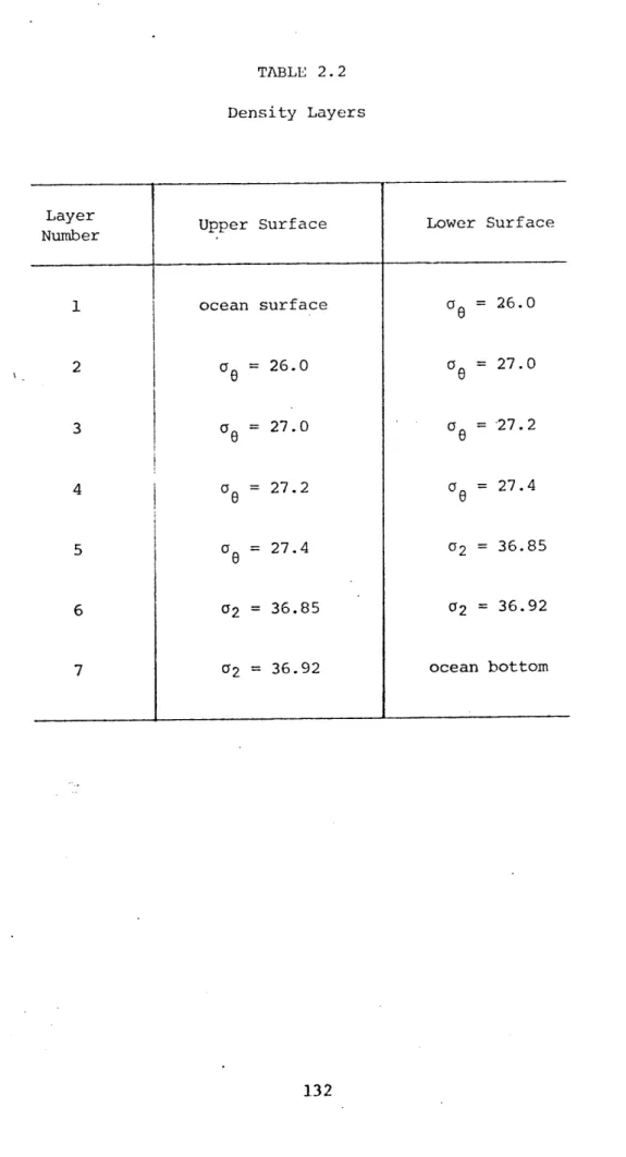
Chapter II The Caribbean Sea .. . . . . . . . . . . . . . . . . . 46

A. Introduction . . . . . . . . . . . . . . . . . ... 46

B. Background _{. . . . 47}

C. Data selection and treatment . . . . . . . . . . . . . . . . 51

D. Results . ... ... ... 52

E. Conclusions . . . . . . . . . . . . . . . . . . . . . . . . 66

Chapter III Gulf Stream '60 . . . . . . . . 69

A. Introduction . . . . . . . . .. . . . . . . . . . . . . . . . 69

B. The integral inverse . . . . . . . . . . . . ... 72

C. The differential inverse ..e *... . .. .... . .. . 74

D. Conclusions . . . . . . . . . . . . . . . . . . . . . . . . 91

Chapter IV Heat flux in the North Atlantic . . . . . . . . . . . . 93

A. Introduction .. . . - -. -. . . . . . . . . . . . . . . . 93

B. The inverse calculation . . . .. 100

C. Results and conclusiofis . . . . . . .. . ... . . . . . 103

Acknowledgements .. . .. . . . 115 Appendix . . . .. . .. . . . . . . . . .. . . . . . . . . . . . . 116 References . . . . 122 Tables . . . . . -. -.- .- . . . 130 Figure Captions . . . . . . . . . ... ... .. . .. .. .. . . 143 Figures . . . . . .. . . . . - . . . . . . ... . . . . . . . . 146 Biographical Sketch . . . . - - -. . . . 192

Chapter I

A. Introduction

This thesis examines the applicability of linear inverse theory to problems in ocean circulation through a series of examples. The method was proposed as being appropriate to the study of ocean circulation by Wunsch(1977,1978), who used it on a hydrographic dataset from the northwest Atlantic. Wunsch's study.established that a multiplicity of

solutions were consistent with the hydrography that he used, with some examples to illustrate the diversity of possible solutions.

A number of important questions about the method formed the

motivation for this work. First, how much more information could be drawn from the data, either by refined data handling techniques or through the imposition of additional constraints? Second, given the strongly

underdetermined nature of the problem st-udied by Wunsch (1978), were there areas where a better determination could be obtained? One might imagine (and later in this chapter a simple example will be given) that hydrography and topography could combine to restrict the admissible

solutions to a fairly narrow range. One would like to know to what extent the range of admissible solutions can be decreased through the addition of data in a given area or through coupling to other areas. A most

important problem, which will be dealt with in each of the applications, is to identify and.interpret quantities that are fully determined by the constraints. This work is about ocean circulation, and an evaluation of the success of the method rests on how much is learned about the ocean.

Chapter I gives a brief review of classical techniques of analysis of ocean circulation followed by a suimmary of the inverse- method formalism as it applies to this problem. This summary is given for the sake of

completeness, and it repeats results that are described more fully in other work on inverse methods such as Wiggins (1972) and Wunsch (1978). The linear algebra may be unfamiliar to some readers and it is hoped that this will not obscure the underlying simplicity of the technique. Two

simple examples are analyzed in some detail, with the intent of demonstrating the principles that can be applied to the more complex problems of the real ocean.

The applications are presented i'n chapters II, III, and IV in the order in which they were computed. The Caribbean Sea was considered first because it was felt that this region, with its strong topographic

constraints and an excellent dataset, would give a clean, unambiguous result. Chapter II describes the solution in that area. Next, it was decided to test the limits of resolution which could be obtained by imposing additional dynamical constraints. Chapter III uses the dense Gulf Stream '60 hydrographic survey for this purpose and a formulation of the inverse problem which is much like the s-spiral method of Stommel and Schott (1977). Chapter IV goes to the opposite extreme in spatial scales. Zonal sections of the Atlantic from the IGY are used to estimate the net transport of heat in the ocean across latitude circles. The three problems are quite distinctive and each presents some.unique features of interest.

B. Background

Classical methods of studying the general circulation using

hydrographic data can be roughly divided into two main categories. One of these is water mass analysis or property analysis. It involves mapping properties such as temperature, salinity, or dissolved oxygen in ways

that are held to reveal the pattern of flow. Wust's core method is one such technique, in which property extrema indicate the 'cores' of various water masses. For instance, the core of Antarctic Intermediate Water is marked by an intermediate salinity minimum, Upper North Atlantic Deep Water by an intermediate salinity maximum, and so on. Wust (1935) mapped salinity, temperature, and oxygen along.a number of core layers in the Atlantic, and used these maps to infer the spreading of water masses. A related method is isentropic analysis, in which properties are mapped along surfaces of constant density. Montgomery (1938) used isentropic analysis to infer the flow pattern of upper waters in the southern North Atlantic. Although these property analysis methods give an indication of patterns of flow, they cannot alone provide estimates of flow volume.

The second type of analysis is the dynamic method. The lowest order dynamical balance for large scale ocean circulation permits the

calculation of vertical shear in horizontal velocity from the horizontal gradient of density. However, integration of shear to get velocity leaves an arbitrary constant, a reference level velocity, unspecified. Many authors have used the dynamic method with some assumption about reference level velocity.

Historically, the problem evolved as an attempt at specifying some surface along which velocity, or a component of velocity, was thought to

be near zero. It was thus referred to as the level of no motion

problem. Sverdrup, Johnson, and Fleming (1942) list four methods (given below) of determining such a level, of which the first three are largely intuitive.

i) Assume that currents are negligible at great depth and

therefore compute current relative to the bottom or to a depth near the bottom. Worthington (1976) found that this assumption led to gross violations of mass conservation in the Northwest Atlantic and therefore did not make geostrophic calculations in the Gulf Stream recirculation region. Instead, he used water mass arguments to close his circulation scheme.

ii) Assign zero velocity to the mid-depth minimum in dissolved oxygen. There is no dynamical or observational support for this method.

iii) (Defant's method) Place the zero velocity surface in a finite thickness layer of minimum shear. Defant (1941) was able to trace this layer over most of the North Atlantic.

iv) Use conservation of mass as a constraint to determine the reference level. Considering the Atlantic as an enclosed basin, any section that spans the width of the ocean should have zero net

transport. The average level of no motion is that depth for which the northward and southward relative transports are equal. Using a pair of Meteor stations near opposite coasts in the South Atlantic, Sverdrup et.

al. (1942) found the level of no motion to be 1325 meters.

In other important work, mid-depth levels of no motion were assumed. Iselin (1936) employed a 2000 meter reference level in his paper on the

circul'ation of the North Atlantic. Stommel's (1965) monograph on the Gulf Stream has dynamic calculations based on a 1600 meter reference surface.

Authors have sometimes used both water mass analysis and the dynamic method, as in Iselin (1936), Montgomery (1938), Worthington (1976), and others. In most cases, the two methods were applied separately, with the results of one being invoked to support, quantify, or question the

results of the other method. The inverse method is in a sense a marriage of the two classical methods because it imposes property conservation constraints in any number of individual water masses, together with dynamic calculations, to estimate a profile of absolute velocity.

Along with the studies mentioned above which apply the dynamic method in order to describe ocean circulation, a number of other attempts have been made to determine the appropriate reference level for such

calculations. Hidaka (1940) selected four stations in the North Atlantic, and by conserving mass and salt in three triangular areas defined by these statons (figure 1.1), was able to write a system of six equations in six unknown reference velocities. Defant (1961) noted that these equations were nearly singular because of the tight T/S

relationship, and the solutions were therefore dominated by noise. This objection would reduce Hidaka's system to three equations in six

unknowns. There are other problems with the method. One can see, for example, that once three of the reference level velocities are specified, then in order to avoid a discontinuity in pressure, the other three can be deduced. On similar grounds, a further reduction in the number of equations can be made.

Stommel (1956) used Ekman dynamics in the surface layer and potential vorticity conservation in the interior to estimate a profile of

meridional velocity from stations in the Sargasso Sea. The vertical velocity at the base of the Ekman layer was computed from measurements of wind stress. This vertical velocity implies a net stretching or

shrinking of the underlying water column. In response, the column must move poleward (for stretching) or equatorward (for shrinking) in order to

conserve potential vorticity. He found a level of no meridional motion which produces the correct net meridional transport. The method left the

zonal velocity undetermined, was applicable only in interior regions where the steady linear potential vorticity equation was thought to be applicable, and ignored vortex stretching due to topography and bottom friction. Sudo (1965) refined the technique by adding a lower boundary condition of no flow across a material surface. Leetmaa, Niiler, and Stommel (1977) used wind stress curl to calculate meridional transport at several latitudes in the North Atlantic. They applied a longitudinal smoothing to remove eddy noise.

Stommel and Schott (1977) obtained an overdetermined system of

equations for horizontal velocity under assumptions of mass conservation, steady linear potential vorticity conservation, and no flow across

density surfaces. Some examples given by Schott and Stommel (1978) showed a sensitivity to noise. A more detailed description of this method is given in the next section and in Chapter

IV.

Many investigators have made direct reasurements of current in order to fix a reference level velocity (c.f. Warren and Volkmann, 1968). Current meters and neutrally buoyant floats have been deployed for this

purpose. However, care must be taken in combining point measurements with spatially averaged valves of shear. One needs a spatially coherent

array of point measurements and one must decide on the appropriate time scale to sample if the measurements are to be used in conjunction with hydrography.

A possible technique for the future is the use of satellite altimetry for the measurement of sea surface height. The slope of the sea surface relative to the geoid is proportional to the geostrophically balanced part of the surface current. At present, errors such as inaccuracies in the estimated geoid are comparable to or larger than the oceanographic signal. If the problems can be overcome, satellite altimetry together with hydrographic data could give absolute velocities over broad spatial

scales with global coverage.

C. The Inverse Method

In this section a derivation of the Wunsch inverse formulation is given followed by a comparison with the related beta-spiral method of Stommel and Schott (1977). These are both inverse methods in the

following sense. The problem'of determining horizontal density gradients from a known geostrophic velocity field can be easily solved by taking a vertical derivative of velocity and then using the thermal wind equation. This.is the forward problem. The corresponding inverse problem is to use a known field of horizontal density gradients to compute geostrophic velocity. Unlike the forward problem, the inverse is non-trivial because of the unknown integration constant.

a). Wunsch's Method

The technique applied by Wunsch (1977, 1978) to the Northwest

Atlantic uses property conservation constraints to estimate the unknown reference level velocity and can be thought of as a generalization of the work by Hidaka (1940) and the fourth method given by Sverdrup, Johnson, and Fleming (1942). It allows the constraints to be- applied to many layers instead of a single layer and permits stable solutions to be calculated in the presence of noisy data.

To begin with, the fluid is assumed to be incompressible and steady so that conservation of mass is given by

V - u = 0 _(1.1)

where

5

bounded on top and bottom by isopycnal surfaces (Wunsch used isotherms) and on the sides by an arbitrary vertical surface S. Integrate 1.1 over this volume and apply the divergence theorem

0

fJv-u

dV'

u -

n dA

+

JJ

u

-

+

JJ

_u

-

_{n dA (1.2)}

V S top bottom

n is a unit vector prependicular to the boundary of V and directed outward. The net flow across isopycnal surfaces is assumed to be negligible so that the second and third terms on the right may be

ignored. The flow perpendicular to the boundary surface S is assumed to be geostrophically and hydrostatically balanced. It can then be

relative velocity computed from the thermal wind equation. u * n = u n = u' n (1.3)

-g

u

n

dA=-

u'

-

(1.5)

Equation 1.5 expresses the fact that no net transport is allowed across the vertical surface S, so that transport due to relative

(sheared) velocity is balanced by an equal and opposite transport due to depth-independent velocity. Ageostrophic transport across S, transport across isopycnal surfaces and transient mass storage within the enclosed volume are assumed negligible. Equations of the type 1.5 may be written for each of a number of layers, or water masses, in a vertical column of ocean. Because the ocean is discretely sampled by hydrographic stations, a discrete form of 1.5 is appropriate for computation. Define the

relative transport in layer i as 1 .. If there are N station pairs of width A x.,

N z

. = u' dz' ) A x. (1.6)

Let x. be the unknown reference level velocity normal to S at station J

pair j.

x. = ( u 'i ).

S 0 J

The area of layer i at station pair

j

a = (separation of pair

j)

Then, the discrete form of 1.5 is

N

a.. x. =(1 7)

j=1 3

If there are M layers, and therefore M equations of this type, the system can be written in matrix form as

A₁XN NX1 MX1

(1.8)

a 1a2 aIN I-y 1

a21 a22 _a

2N

or .

-aM1 aM2 aMN

In addition, adjacent volumes of ocean with common bounding surfaces can easily be included in coupled systems of equations. If the data were

perfect and the physical assumptions were precisely correct, then one could imagine increasing the number of water masses until the number of equations was about equal to the number of unknowns. However, small

amounts of noise obscure differences between equations that are almost linearly dependent, and reduce the effective number of equations (rank of A).

b. The method of Stommel and Schott

The beta-spiral inverse of Stommel and Schott (1977) is given in differential form. As noted by Davis (1978), the physical assumptions

are much the same as in Wunsch's integral formulation. One assumes

continuity (1.1), geostrophic and hydrostatic balance, and no flow across isopycnal surfaces written as

u h + v h w where for example h-

-

x y x x] Pz

Then, the further explicit assumption of a linear steady potential vorticity balance is

v = f w (1.10)

z

These assumptions are presumed to be valid for large scale (0(1000 km)) flows in the ocean interior, so the data should be appropriately

smoothed. The equations are combined to give

u h + v (h - 6/f) = -u' h - v' (h -

s/f)

o xz 0 yz xz yz

When written with data from many depths, the system of equations is formally overdetermined. For comparison, a differential form without using 1.10(equivalent to the Wunsch formulation) is obtained by taking a z-derivative of 1.9 and then substituting for w from 1.1.

u h + v h + u + v -(u'h - v'h -u' -v'

)

o xz o yz ox oy xz yz x y

Note that there are four unknowns, u ,x v0,, u0, and v rather

than 2 as in 1.11. Writing this equation with data from many depth produces the following coefficient matrix A.

h (z

)

)

xz 1 yz 2

h (z

)

)

xz m yz m

One can see that this matrix is at most of rank 3 since the third and fourth columns are identical. The system of equations is underdetermined without the vorticity balance. However, computation of u' + v' y

using geostrophy gives f , and for consistency one should set u +

ox

Ovo

Voy equal to . The result is of course the beta-spiral equation 1.11. This is Davis' (1978) point. In the mid-ocean case, with no topography, the two methods are equivalent if the implicit use of 1.10 is recognized.

It will now be shown that in a more general application of the

integral formulation, the equivalence does not hold. The key step is the use of the divergence theorem. Note that in the interior of the volume V, only continuity (1.1) is assumed. Any vorticity balance is

permitted. The use of the steady linear vorticity balance is only implicit only if the hydrographic sections completely enclose the area and if there is no topography. If there are land boundaries or

topography, then the argument advanced in the last paragraph no longer applies. Indeed, deviations from the steady linear balance, 1.10, will contribute to the signal, as we shall see.

An example makes the point clearly. Consider a 2-layer

representation of a zonal section of the North Atlantic, as in Stommel, Niiler, and Anati (1978). They note that the thermocline is deeper at the _{eastern boundary than at the western boundary. This implies (in the} 2-layer model) a net northward flow of the upper layer relative to the lower layer. Examination of isopycnal surfaces ranging from ag = 27.1 to 27.7 in the IGY section at 300N shows an average net drop of roughly 200 meters from west to east. Isotherms drop by much more, because of variations in TS characteristics approaching the Mediterranean outflow. Considering the North Atlantic as a closed basin, one could trace the a =27.4 surface along the boundary from Spain around to North America and find a net upward slope. Pressure gradients along the coast in one or both layers must accompany this slope. With no steady flow into the. coast, these very small pressure gradients are not geostrophically balanced. They reflect the accumulation of small non-geostrophic terms in the momentum balance.

Scale analysis shows that this is not unreasonable, since effects of the proper magnitude can be produced by a low Rossby number flow. For instance, suppose part of the alongshore pressure gradient is balanced by deceleration of the western boundary current above a lower layer at rest, with the pycnocline slope along shore compensating for slope of the sea surface. Assume, for scale purposes, a pycnocline height change of 102 meters in a distance alongshore of order 106 meters, with a

characteristic current speed of 1 m/sec and a density difference A of 1 p

x 10-3. Then the ratio of advective acceleration to Coriolis acceleration is very small.

U U

x gAP .01

fU pfU L

The point here is not to quantify the vorticity balance, which may vary in a complicated way in space and time, but merely to observe that other balances besides 1.10 are consistent with the integral formulation of the inverse. Without the net pycnocline slope in the preceding example,

there would be no imbalance in the baroclinic mass flux and one could not then infer a barotropic circulation, as is done in Stommel et al. (1978) and more generally in the Wunsch type of inverse problem. Resolution is greatly improved by the use of an appropriate vorticity equation as in Stommel and Schott (1977). An example of this increased resolution is given in chapter IV using the dense sampling of the Gulf Stream '60 experiment.

The question of how much information to include in a problem, whether the information is in the form of data or physical relationships, is one of resolution versus stability. As one includes more independent

information, problem resolution improves. If, however, the added information differs from other information only in noise content (data noise or inappropriate physics) then no additional resolution is

achieved, and to force the problem to be more highly resolved simply decreases the stability of the solution. This tradeoff is really the key to the whole problem and is discussed in more detail in the subsequent sections on resolution, weighting, and noise.

The matrix equation 1.8 can be solved by a singular yalve

may be found in Lanczos (1961), Wiggins (1972), Wunsch (1978), and other sources. One can always write the matrix A as the product of three matrices

XNUMXK XK XT (M < N) (1.12)

The columns of the U and V matrices are orthonormal.

UTU = I and VTV = I but, in general VVT /I and UUT I

The matrix L is a diagonal matrix of the non-zero 'singular values'. U and V are the respective eigenvector matrices for the eigenvalue problems

T 2 T 2

(A A ) u = 1 u and (A A) v = 1 v

The non-zero eigenvalues, 1 2, are the same for both of these problems and they are the squares of the 'singular values' in matrix L. Since standard numerical routines are available to compute eigeivalues and eigenvectors of square matrices, the SVD of the rectangular

matrix

easier to solve the first of the above eigenvalue problems than the second. This gives U and L, and V is calculated from 1.12

VT = L UTA

-1 T

The SVD solution to 1.8 is obtained by left-multiplying 1.8 by VL U

V L UTA x = V VTx = -V L U F (1.13a)

Define b = VV x and note that

Therefore b (the SVD solution) is in fact a solution to 1.8. The 'correct solution', that is the solution that would be obtained if the

T

resolution was perfect (i.e. if rank(A)=N so that VVT=I) ,is denoted by x, whereas the estimate of x is called b. Of the infinity of possible solutions to 1.8, the SVD solution is the smoothest in the sense of introducing no structure that is not necessary to satisfy the

constraints. _{In the ocean circulation problem, this means that the} largest available scales in the data are used and the reference level velocity is smoothed over these scales.

If the matrix A has K linearly independent rows (rank (A) = K), then only K of the singular values are non-zero. In practice, because of noise in the A matrix, singular values that should be zero are instead small positive numbers. One must rank the singular values from largest to smallest and decide beyond what value they should be considered to be equal to zero. Wiggins (1972) discusses several techniques for making this decision. One may either take what he refers to as a sharp cutoff or a tapered cutoff approach. In the former, small singular values (and their corresponding eigenvector coefficients) are excluded from the solution in order to hold down the problem variance. In the latter, the effect of small eigenvalues is damped by replacing 1.8 by

Ax + n = - r (1.14)

2 2

problem variance. The tapered cutoff solution to 1.14 is

b = A T (AA + I) (- ) (1.15)

-2

Here, a is the ratio of the problem variance to the solution -2

variance. Wiggins(1972) shows that the effect of G is to eliminate the effects of the smallest eigenvalues. Hoerl and Kennard (1970 a,b)

-2 studied the behavior of the length of the solution vector as CJ is

varied, a technique termed ridge analysis. A discussion of this inverse and its relationship to the SVD inverse is given by Wunsch(1978).

The examples in chapters II, III, and IV use both the sharp and tapered cutoff methods. For sharp cutoff, the decision on the smallest non-zero singular value was made by studying estimated error variance, length of solution and residual vectors and smoothness of the VV

matrix (discussed in the next section) for several choices of K. Usually the smallest singular value was about 2 orders of magnitude less than the largest. The solutions tend to be very stable with respect to small changes in K.

D. Resolution

The non-uniqueness of solutions to the problem 1.8 leads to the question of how to interpret a particular solution b _ . The

j

infinity of possible solutions are all compatible with the imposed

physics. All must be considered possible states of the real ocean until additional data or further constraints are introduced. However, a set of K independent linear equations does give a unique determination of K linear combinations of the solution elements. It is the purpose of this

section to show that in some problems, these well determined quantities have a simple and physically useful interpretation.

An example brings out the main points. Consider a 2-layer ocean bounded by land on the north and south. Two hydrographic sections

containing 2 and 1 station pairs traverse the ocean. Figure 1.2 shows the geometry, with areas of upper and lower layers marked at each station pair. Let the A-matrix be composed of areas of the upper-layer (1st row) and of the total water column (2nd row).

.5 .4 .4

A

:

1.0 .9 .4

For now, ignore the question of weighting and assume A is noise free so that its rank is 2. The singular value decompositioni of A is given by

T _ .4659 .88481 1.583 0 .7060 .6207 .3411] .8848 .4659 0 .1814J 1 .1311 .3589 -.9241

Define a matrix R, called the resolution matrix

T{.5156 .4853 .1197

R VV .4853 .5141 -. 1199 (1.17)

.1197 -. 1199 .9703

Wiggins (1972) shows that the columns of the resclution matrix

represent the best approximation, in a least square cerror sense, to a set of delta functions, 6.. The columns measure the degree to which

individiual station pairs can be resolved using line-Ar combinations of the eigenvectors. They cannot ,in general be perfectly resolved because the V-eigenvectors only span the observation (row) space of A and not the solution (column) space, which is of higher dimensioni.

The indeterminacy can be examined directly by computing the vector which is orthonormal to the two V eigenvectors in 1.16. In general there

are N-K such vectors. They are called the null-space eigenvectors, or annihilator of A, because they are normal to the rows of A. In the example, the null-space eigenvector is

v3 = (.70,-.70,-.17)

The infinity of possible solutions will differ from each other by

multiples of v₃. That is, given any solution, an arbitrary multiple of v3 may be added to that solution and the result will still satisfy the

constraints since v3 has no effect on the constraints. One can see that v is primarily a recirculation between station pairs 1 and 2 (v =

3 13

-v23 ). The extent of this possible recirculation is the undetermined quantity in the problem.

A second interpretation of R follows from 1.13. Suppose,

hypothetically, that the reference level velocities in the ocean were somehow known at each station pair. This set of velocities will be referred to as the 'perfectly resolved' solution. Then, according to 1.15, multiplication of these velocities by R would produce the SVD solution, b. The resolution matrix is a linear operator which maps the perfectly resolved solution (as well as every other possible solution) into a particular solution b. It is a filter for which the real ocean is the unknown input and the b's are the computed output.

In the example, 1.16, if the perfectly resolved solution was

1

by the first column of R, would be b ₁ = .5156, b ₂ = _.'3.4853, b =

.1197 . _{Similarly, the second and third columns of R give the computed}

solutions _{which would result if the perfectly resolved solutions were} (0,1,0) and (0,0,1) respectively. Because the system is linear, such solutions may be added. It is obvious that station pair 3 is well resolved by itself. Pairs 1 and 2 are not well resolved individually, but are well resolved as a group. Any velocity in either of these pairs

is simply smoothed over _{both, with minor 'spillage' into pair 3. In this} case, R is a good spatial averaging filter, with the averaging pretty well confined to the separate sections. In such instances, where physically adjacent groups of statibns are resolved, the resolution is said to be compact. A problem with non-compact resolution can be

constructed trivially by considering station pair 2 to be one section and pairs 2 and 3 combined to form the other. The resolution matrix is unchanged, but now, since pairs 1 and 2 are no longer physically adjacent, the resolution is not compact.

The resolution of volume transport is often a more useful quantity than the resolution of velocity because the constraints are written in terms of transport. _{Whereas velocity need not be preserved by the} operator R, as in the case of groups of stations of very different

widths, transport must be conserved for the constraints to be satisfied. A matrix for resolution of volume transport due to the reference level velocity, say in the ith layer, can be obtained by multiplying the

corresponding velocity resolution elements by the appropriate water mass area (element of the A-matrix) and then normalizing.

Suppose, for example, that one wants to know the amount of transport that will appear at station pair 2 because of the failure to p)erfectly resolve station pair 1. Let row i of the A matrix represent the total transport constraint. The velocity resolution element r_{2 1} gives the velocity at station pair 2 that results from imperfect resolution of a velocity of 1 at station pair 1. Then r2 1 a.2 converts this to a

transport at pair 2. Finally (r a )/a is the transport at pair

21 i2 il

2 due to the imperfectly resolved transport (instead of velocity) of 1 at pair 1. More generally,

r . a.

t = a .P (1.19)

pj a j

In the example, the resolution matrix. for total transport is

.5156

.5392

.2993

T .4368 .5141 -. 2698 (1.20)

.0479 -. 0533 .9703

Note that the sum in any column is 1 so transport is conserved.

Inspection of this matrix suggests that computed net volume transport in each section will probably agree with the real transports to within about 5%.

Although the example problem is formally underdetermined, good

estimates have been obtained of-net transport through each section and of the smoothed reference level velocities. Indeed, the only thing not determined is the extent of the possible recirculation .between station pairs 1 and 2. With good hindsight, one can look back at the A matrix

and see that the resolution agrees well with intuition. Station pairs I and 2 have nearly the same proportions of shallow and deep water. It is this purely geometrical similarity which leads to their being grouped

together. They are geometrically almost indistinguishable, and therefore they will be assigned nearly the same solution elements. Station pair 3 is distinctly different by virtue of having no deep water. It is

therefore well resolved by itself.

What if, because of noise, the rank of A is found 'to be 1 rather than 2? With only one independent equation, all three station pairs should be grouped together.

.50

The relatively small velocities and transports at station pair 3 are due to its small area in the unweighted problem. Notice that the sum of the columns in the transport matrix is not as close to 1 as in the K = 2 case. As the constraints are relaxed, transport is not as well conserved by the smoothing operator.

The kind of reasoning applied to this simple problem can also be used in real problems to anticipate resolution. That is a central question of Chapter II. In general, station pairs with similar ratios of layer

depths will be grouped together in the solution. More precisely, groups are formed from station pairs whose corresponding columns in the A-matrix are most nearly linearly dependent. If the station pairs are physically adjacent, then the resolution is compact, the solution is a spatially smoothed version of the real reference level velocity field. Salt

.50 RK = .44 .24 .44 .24 .39 .21 .21 .12

advection, heat advection, etc. (assuming a tight T/S curve) can be estimated for the groups. If the resolution is not compact,

interpretation is far more perilous.

The essential difference between compactness and non-compactness is easily illustrated. Consider a slice of ocean bounded by two

hydrographic sections that run from a coastline to a common point in mid-ocean (Figure 1.3a). Suppose that each section has many station pairs but that out of all station pairs, two have identical depths and layer thicknesses. The corresponding two columns of the A-matrix will be equal and the solution elements for the two stations will be equal in terms of the mass flux constraints. That is, if the two station pairs are in opposing sections, the determined velocities will be equal and opposite (Figure 1.3b). If they are in the same section (say side by side), the determined velocities will be equal and of the same sign (Figure 1.3c). The indeterminate part of the flow is any flow that does not affect the mass flux constraints. This null space of A admits, in the first case, the possibility of an arbitrarily large mass flux through the system, so long as it is the same at the two station pairs (Figure 1.3d). In the second case, the undetermined quantity is simply a small scale recirculation in the adjacent pairs (Figure 1.3e). An example of the first type will be shown in Chapter IV using Gulf Stream '60 data and one of the second type in Chapter II on the Caribbean Sea.

We have shown that, in the compact resolution case, the b's represent a spatially smoothed version of the reference level velocities. However, the choise of reference level is somewhat arbitrary, and further, a display of the smooth b's together with unsmoothed relative velocities

entails a mismatch in scales. The relative velocities each represent an average over a single station pair while the b's are typically averaged over many station pairs. The mismatch is removed simply by applying the same filter to the relative velocities as was applied to the reference velocities. At each level,

(VVT) (vr) v

NXN NX1 NX1

The total smoothed velocity is then

(vr + b)=VV vr+x) (1.21)

The smoothed field is independent of the initial reference level, since every level has been filtered by the same operator. In this sense the

smoothed field is unique. Further, the smoothed field gives, at every level, the b field which would result if that level were chosen as the initial reference level in the computation of an unsmoothed solution. This means that one need not recompute the SVD solution for each choice of initial reference level. A single computation of the smoothed field gives the b's corresponding to each initial reference level. The formulation of the smoothed field (1.21) is equivalent to the more complicated appearing form given by Wunsch (1978).

E. Weighting

In the applications discussed in Chapters II, IT, and IV, the unweighted problem, 1.5, is replaced by the weighted problem.

''' -1/2 ' +1/2 _(.2

A b =-FA =AW b =W b (1.22)

There are two purposes for this substitution. One is to remove any unintentional bias in the solution. The other is to impose a bias by controlling the solution variance or influencing the problem resolution.

Hidden bias in the ocean circulation problem is the result of different station pairs having different areas (product of mean depth times station separation). Consider two adjacent station pairs with the same mean depth and the same layer thicknesses, but whose station

separations differ by a factor of t. The solution should not be

sensitive to the placement of the center hydrostation (i.e. to the value of a) and should clearly be the same at the two station pairs. The

matrix A will show two columns that differ only by a factor of a. If the station pairs are at positions

j

a.. aa.. 13 .13 A = a .aa 2j 2j a . eaa mj mj

The V eigenvectors, which span the rows of A will have elements that differ by a factor of a

V e=

T

11

11

V. aV. jk jk

The corresponding columns of the resolution matrix also differ by the factor a K K r.

_ij+l

j+11

31

The solution elements, which by symmetry should be equal, show the same bias\.

b = (..b., a b.,..

)

J J

The symmetry argument is not quite as compelling when applied to depth. Suppose two station pairs have the same separation and the same ratios of layer thickness to total depth for each layer, but that the depths differ by a factor of c. Once again the solutions are biased as above. However, it is not obvious that the same solution should be assigned at both station pairs. For one thing, this hypothetical situation does not occur in the real ocean, where shallow stations may show less "of the dense layers without having thinner upper layers. Nevertheless, it is undesirable to assign a large velocity to a deep

station merely because it is deep, so removal of all bias based on the area of station pairs seems reasonable. This is accomplished by setting

W.. = 6.. (d. Ax.)1 (1.23)

In the weighted problem,

,

~

1/2 1

1

2a

Next, the weighting is removed from the resolution matrix in order to derive an expression analagous to 1.13. Let

A' = U L VT

T -1

-VV X' = VL U TA'X' = VL U T = b'

so b = (W-1/2 T +1/2) X

Define, R = W-1/2 T +1/2

_(1.24)

R can be called the deweighted resolution matrix. It is easily verified that in any column of this matrix, the two elements corresponding to the two hypothetical station pairs are equal, i.e.

r.l . = r

Application of the weighting scheme 1.22 to the earlier example 1.16 improves the resolution of station pair 3 (the smallest in area) by cutting down its side lobes. Compare to 1.17 and 1.20.

.48 .47 .05 .48 .52 .13

r . a.

R .52 .53 -. 05 T = .47 .53 -. 12 (t = ) (1.2

.13 -. 12 .99 .05 -. 05 .99 3

5)

The weighted problem is also useful if there is anything known about correlation length scales of the velocity field or if it is desired to force certain solution elements to be correlated. _{The weight matrix W is}

the covariance matrix of the solution elements, b (Wiggins, 1972). The use of non-zero off-diagonal elements in this matrix causes corresponding solution elements to be correlated.

Refer again to example 1.16. Suppose that the mass imbalance is given by

r

[10

10

The lower layer is balanced, but the upper layer (and therefore the total water columnn also) has a mass surplus. There are two ways of balancing the system. An outflow velocity at station pair 1 coupled with an equal inflow velocity at station pair 2 gives a net outflow of upper water and no net flux of deep water. Alternatively, an outflow at station pair 3, which has no deep water, accomplishes the same end. Solutions consistent with these two extremes are

100 0

i) b= -100 ii) b= 0 (1.26)

0 25

Using the simple diagonal weight matrix, 1.23, the SVD solution is

1.3

b = W1/2 U,TSg, I' = -1.3 (1.27)

24.7

The second alternative is favored by the SVD solution since it gives a much lower value of b b. However, the SVD solution can be driven

closer to either 1.26i or 1.26ii by imposing non-zero covariances. If an off-diagonal element of W-1/2 is set equal to a diagonal element of the

same row, the corresponding two solution elements are perfectly correlated. In other words, if

W W and W W

12 11 21 22

then, this is equivalent to the additional constraint b _{= b2} Similarly W12 " -W11 and W21 22 leads to bl ₌ -b2

The former leads to solution 1.26ii and the latter to 1.26i. As the off-diagonal elements go from zero to plus or minus the value of the diagonal elements, the whole range of solutions between 1.27 and 1.26ii

or 1.26i is accessed.

Similar alternatives exist in real problems where large eigenvalues are associated with broad flows that account for most of the mass

balance, and smaller eigenvalues bring in smaller scales, particularly small scale recirculations that make minor adjustments in the net flux of mass. An approach advocated by Jordan and Franklin (1968) attempts to enhance the resolution of the broad scales by solving the problem first with a diagonal weight matrix to determine what solution elements tend to be grouped in resolution, and then repeating the problem with positive covariances between members of each group. According to Wiggins (1972),

this will cause the eigenvalues to become more polarized, with large ones becoming larger and small ones becoming smaller. The intended effect is

to put more emphasis on the best determined, least noise sensitive components of the ~solution.

It is quite possible to become bogged down in details of a weighting scheme, and some perspective is useful. One can never obtain the

velocity field with perfect resolution. Rather, one can derive a filter, R, and also the unique output of this filter after it acts on the true velocity field. Interpretation of the output relies on the filter having

some relatively simple characteristics. It should perform a local spatial smoothing. The weight matrix is the means of manipulating the filter (to a limited extent) to perform the desired function.

In addition to the column weighting, it is also posssible to perform a row weighting in order to vary the weight placed on each constraint in

the problem. Let

A' 1/2 '' 1/2 ' so that A b' =-P If '' T A U L V T

then the singular value decomposition solution is

and

b = -W-1/2 V L~ UT S1/2 F

Wunsch (1978) discusses this row scaling. The matrix S

1

F. Errors

Error estimates for problem 1.8 are made either by considering the size of errors in the observations or from a study of problem residuals (goodness of fit). The two should be comparable in magnitude. If they are not, then either the observational errors are incorrectly assessed or the physical model is insufficient to describe the data. The following begins with a discussion of errors in the data. Some comments on likely errors in the model are made, and then briefly, the propagation of data errors through to the solution is considered.

1. Data Errors

A hydrographic station in deep water normally consists of two Nansen bottle casts. A shallow cast is made with about 12 to 15 bottles at 100 meter intervals (or closer near the surface). The bottles should be

placed to be as close to standard depths as possible in order to minimize interpolation errors in dynamic computation. Except in regions of high shear (resulting in large drag dn the wire), the bottles can usually be placed within 10 to 20 meters of optimal depth. In the deep cast, bottle spacing may be 200 to 300 meters or even greater at very deep stations. Interpolation errors are small below the thermocline where the vertical

profiles of temperature and salinity become almost linear. The

'artistry' of a deep cast is in placing the bottom bottle as close as possible to the ocean floor.

There are measurement errors in temperature, salinity, pressure, and geographical position (navigation). _{The magnitudes of the first three,} for carefully made Nansen casts, is roughly .020C in temperature, .005%. in salinity and 5 decibars in pressures up to 1000 decibars and about .5%

at greater pressure. Navigation errors depend on the method used (e.g. Loran, satellite, etc.) but are usually negligible in relation to the other errors. An equivalent error in the pressure of a given isopycnal can be estimated by multiplying the position error by isopycnal slope. An error of 1 kilometer, even with a relatively large isopycnal slope,

say 1 x 10-3 , is equivalent to only 1 decibar in pressure.

The interpolation procedure for temperature and salinity is discussed in the Appendix along with other details of computation. Some tests of the interpolation routine using CTD data with dummy 'observed' depths showed that in most cases the interpolation errors were smaller than, or the same size as, the measurement errors. Exceptions were at depths where there is both large curvature in the vertical profiles (usually the upper 1200 meters) and where the interpolated depth was nearly midway between observed values. _{Then rms errors of about .08} 0_{C in temperature}

and .015%0oin salinity were found. _{Internal waves with displacements of} order 10 meters give rise to errors of equal or smaller magnitude than those due to measurement and interpolation.

The equation of state gives specific volume as a function of salinity, temperature, and pressure. Given specific volume at two adjacent stations, A and B, vertical shear is computed from the

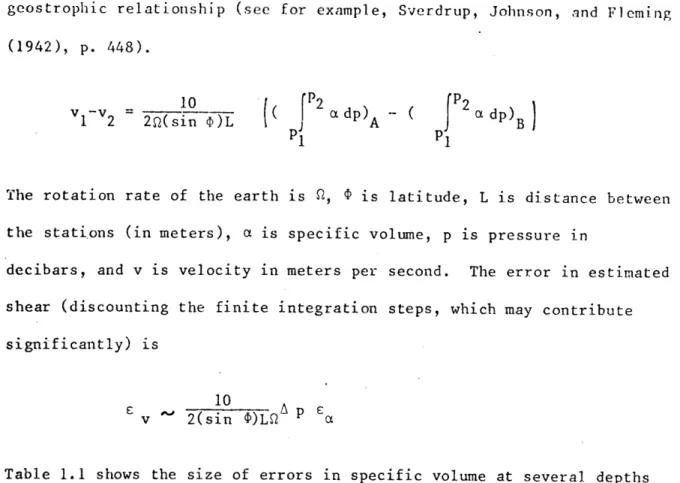
geostrophic relationship (see for example, Sverdrup, Johnson, and Fleming (1942), p. 448).

10 f2 2

v -v _{1 2} = _20(sin 0 _t)L

V

1 1

The rotation rate of the earth is Q,

_#

decibars, and v is velocity in meters per second. The error in estimated shear (discounting the finite integration steps, which may contribute significantly) is

10 A

v ^' 2(sin )LD2 a

Table 1.1 shows the size of errors in specific volume at several depths from Crawford station 889 (in the Sargasso Sea), computed by assuming the measured temperature, salinity, and pressure to be in error by .020C,

.005%9 and 5 decibars or .5% (whichever is greater) respectively. From this, a rough estimate of error in relative velocity is obtained for a station pair at mid-latitude with a separation of 100 kilometers, a depth of 4000 meters and a typical specific volume error of 1 x 10-5

3

cm gm. The error in relative velocity accumulates with the number of integration steps away from the reference level to 0(1 cm/sec). The corresponding uncertainty in the relative volume transport is about 2 x

6 3

10 m /sec. Thompson and Veronis (1978) calculated the error in relative transport assuming random errors in the measurements with standard deviation .005% in salinity, .02

0C

pressure for a data set in the Tasman and Coral Seas. The estimate of 4 6 3

x 10 m /sec was mainly in the deep water.

In the preceding, there are several important points which are somewhat obscured by the numbers. First, transport errors are latitude dependent, with a singularity at the equator. Errors in adjacent layers may be strongly correlated. That is, an error at any standard depth is

carried over into all subsequent standard depths. Finally, since the relative total transport through a section is dependent only on the end stations, the estimated error is the same for any section (except for the latitude dependence) regardless of length and number of station pairs, and is equal to that for a single station pair.

Aside from the errors which result from measurement and

interpolation, there are additional errors in the presence of a sloping bottom, due to the lack of data along the bottom. Below the deepest bottle of the shallower of two stations, there is no accurate way of determining shear. _{Historically, methods such as those of Helland-Hansen}

(1934) and Jacobson and Jensen (1926) were devised to estimate shear (and sometimes absolute velocity) along a sloping bottom. The physical

assumptions of these methods are difficult to justify. Wunsch (1977) filled in values for shear below the deepest common standard depth by a linear vertical extrapolation of shear. This proved unsatisfactory in cases where the shallow station was in the thermocline and the deep station much deeper, resulting in unreasonably large values of relative velocity. Some experimentation with simple horizontal and vertical extrapolations of the measured fields showed the former 'to be slightly more stable. However, a vertical procedure, in which isopycnal slope was

held constant below the deepest common standard depth, was settled on here. It seems clear from studying open ocean sections of temperature and salinity that the vertical coherence of the fields over several

hundred meters is visibly greater than horizontal coherence over station spacing scales (20 - 100 kilometers). Thompson and Veronis (1978) also used a vertical method, requiring shear to diminish linearly to zero at the bottom.

Lacking sufficient observations to predict the behavior of the

density field near sloping boundaries, any method is prone to significant errors. The errors are probably comparable to the actual shear, and therefore range from a few tenths of a centimeter per second for depth differences of a few hundred meters in deep water to tens of centimeters per second for depth differences of a couple thousand meters in energetic regions. The resulting error in relative transport depends largely on whether or not the reference level is the bottom. If the reference level is above the deepest common standard depth, then the shear error

contributes to transport error only below the deepest common standard depth. If the reference level is the bottom, then the deep shear error leads to a relative velocity error in the whole water column. For

example, suppose station A has a depth of 1000 meters and station B has a depth of 2000 meters. Let the velocity error be linear from 1000 to 2000 meters and equal to 5 cm/sec at 1500 meters. If the station separation

is 25 km (stations are normally fairly close over steep slopes), then a bottom reference level leads to a transport error of about 3 x

106_{m3/sec while a reference level at 1000 meters gives an error of} 6 3