HAL Id: tel-01086451
https://tel.archives-ouvertes.fr/tel-01086451
Submitted on 24 Nov 2014HAL is a multi-disciplinary open access archive for the deposit and dissemination of sci-entific research documents, whether they are pub-lished or not. The documents may come from
L’archive ouverte pluridisciplinaire HAL, est destinée au dépôt et à la diffusion de documents scientifiques de niveau recherche, publiés ou non, émanant des établissements d’enseignement et de
Alice Pisani
To cite this version:
Alice Pisani. Cosmology with cosmic voids. Cosmology and Extra-Galactic Astrophysics [astro-ph.CO]. Université Pierre et Marie Curie - Paris VI, 2014. English. �NNT : 2014PA066240�. �tel-01086451�
Sorbonne Universit´es
´
Ecole doctorale d’Astronomie et
Astrophysique d’ˆIle-de-France (ED 127)
Institut d’Astrophysique de Paris (IAP)
Cosmology
with Cosmic Voids
Par Alice Pisani
Th`ese de doctorat de Cosmologie
Dirig´ee par Benjamin Wandelt (Chaire Internationale `a l’UPMC)
Pr´esent´ee et soutenue publiquement le 22/09/2014Devant un jury compos´e de (par ordre alphab´etique):
Pr. James Bartlett APC Examinateur
Pr. Val´erie de Lapparent IAP, CNRS Invit´ee
Dr. St´ephanie Escoffier CPPM, CNRS Rapporteure
Pr. Luigi Guzzo INAF Examinateur
Pr. Michael Joyce LPNHE Examinateur
Pr. Rien van de Weygaert Kapteyn Institute Rapporteur
Introduction 4
1 The large-scale structure of the Universe, cosmic voids, and
the pillars of Cosmology 7
1.1 Historical overview of the large-scale structure discovery . . . 8
1.1.1 Looking outside our galaxy . . . 8
1.1.2 1976: first surveys . . . 10
1.1.3 The discovery of cosmic voids and the large-scale structure 12 1.1.4 The large-scale surveys . . . 16
1.2 An abridged history of Cosmology . . . 19
1.2.1 The pillars of Cosmology . . . 20
1.2.2 Friedmann equations . . . 27
1.2.3 Distances . . . 31
1.3 Recent developments in Cosmology . . . 40
1.3.1 Our Universe . . . 43
1.3.2 The most boring Universe? . . . 50
2 Understanding the Universe with Voids 54 2.1 Standard objects . . . 55
2.2 Cosmic voids . . . 60
2.2.1 Voids as a tool for dark energy . . . 63
2.2.2 Alcock-Paczy´nski test with voids . . . 65
3 Redshift space distortions: To real space and beyond 71
3.1 Redshift-space distortions . . . 71
3.2 To real space . . . 73
3.2.1 Using sphericity . . . 73
3.2.2 Notation . . . 75
3.2.3 The inverse Abel transform . . . 75
3.3 Ill-conditioning . . . 77
3.3.1 Polynomial regularisation . . . 77
3.3.2 Singular value decomposition . . . 79
3.3.3 Di↵erences between the methods . . . 80
3.3.4 Technical details . . . 81
4 Testing void reconstruction 83 4.1 The ideal case: no-noise . . . 83
4.2 The toy model: constructing and using a simple benchmark . 86 4.3 Dark matter particles . . . 90
4.3.1 Reconstructed density profile of a stacked void with the polynomial regularisation method . . . 91
4.3.2 The reprojection, a quality test for the reconstruction . 95 4.3.3 The singular value decomposition method for the simu-lated void . . . 96
4.4 Galaxy mocks . . . 97
5 Results: real space density profiles for stacked voids from SDSS DR7 101 5.1 Results . . . 101
5.2 Discussion . . . 109
5.3 Possible direct applications . . . 111
5.3.1 Mass compensation and theoretical prediction of veloc-ity profile . . . 112
5.3.2 Velocity reconstruction . . . 121
6 The effect of peculiar velocities and VIDE 126 6.1 VIDE . . . 128
6.2 Peculiar velocities a↵ect voids and VIDE . . . 131
6.2.1 Simulation and HOD details . . . 131
6.2.2 The matching algorithm . . . 132
6.2.3 One-to-one comparison . . . 133
6.3 Results . . . 134
6.3.1 Matched fraction . . . 136
6.3.2 Average ellipticity variation due to peculiar velocities . 140 6.3.3 Guidelines . . . 144
6.4 E↵ect of velocities on HOD stacks . . . 145
6.5 Discussion on peculiar velocities . . . 147
7 Constraints from cosmic voids: Alcock-Paczy´nski test and abundances 149 7.1 Recent Alcock-Paczy´nski test application . . . 150
7.2 Constraints from void abundances . . . 152
Conclusion 159
Acknowledgements 162
Appendix A 166
Appendix B 170
Bibliography 173
Cosmology is the science that studies the Universe as a whole, with the objec-tive of explaining its structure and evolution. To reach information about the Universe, one way is to observe the largest scales possible, considering galaxies — groups of stars bound by gravity — as points, and tracing their positions and movements. The large-scale movement of these tracers tracks for us the evolution of the Universe. At large scales, clusters of galaxies, sheets, voids and filaments shape the Universe –– it is the Cosmic Web.
While most of the work to understand the large-scale structure of the Universe has focussed on the over-dense regions, emptier regions are gaining interest: cosmic voids, discovered in 1978, are the under-dense regions in the Universe, with sizes from ten to hundreds of Mpcs.
Until very recently, due to the difficulty of extracting data from low den-sity zones, the potential of voids has been under-explored. Modern surveys allow us now to access to high quality large-scale-structure measurements, by sampling the galaxy distribution in great detail also in sparse regions: the appeal of cosmic voids becomes thus considerable.
Being devoid of matter, cosmic voids might be mainly composed of dark energy — which strongly justifies their importance for Cosmology, as dark energy is believed to be 70% of the Universe and we still do not understand it. The e↵orts of cosmologists seem to converge to a cosmological model (called ⇤CDM) that leaves many unknowns. The nature — and we could say even more, the existence — of dark energy remains a mystery; and so does the nature of dark matter. In this framework cosmic voids appear as a new potential probe for our quest of a correct model for Cosmology.
Cosmic voids fill most of the Universe, and have simpler dynamics than high density regions of the Universe. As such, they constitute a promising laboratory to test dark energy, constrain cosmic expansion and discriminate between cosmological models such as modified gravity models. Despite of being simpler, Cosmology with cosmic voids is only at its commencement. In the era of precision Cosmology, each cosmological probe needs a careful understanding of the systematic e↵ects a↵ecting measurements and, to become competitive with other probes, requires detailed study. Aiming to constrain cosmological parameters with voids, we need to ensure that we are able to correctly understand and model them.
The use of voids to constrain Cosmology is based on studying their shapes, their number density and their evolution. These properties are indeed depen-dent on the cosmological model and can thus be used to constrain it. In this framework the major source of systematics is the presence of peculiar velocities.
When we observe cosmic voids, we observe them in redshift-space: their real shape remains inaccessible to us, thus greatly limiting our knowledge about such structures. To employ voids as a precision tool for Cosmology, it is fundamental to obtain their real shape and eventually to understand how peculiar velocities a↵ect them.
The purpose of this thesis is to find a model-independent way to access the real shape of the voids, i. e. the real-space information, adopting as few assumptions as possible about the cosmological model. This work aims to answer to the following questions: how can we extract real-space information from cosmic voids in a model-independent way? Can we understand the sys-tematics in the use of cosmic voids? Can we obtain real-space information from real data? The application of any method we consider to real data it another fundamental point of this work: as voids are to be used as cosmolog-ical probes, we cannot disentangle us from real data, which have the ultimate word in assessing the quality of models. Furthermore, using realistic HOD models mimicking real data, it is possible to study the major systematics af-fecting the use of voids as cosmological probes: peculiar velocities. Obtaining
the real-space shape of voids and understanding how velocities a↵ect our mea-surements are crucial steps towards the goal of precision-level Cosmology with cosmic voids.
Chapter 1 presents the large-scale structure of the Universe and the discov-ery of cosmic voids, as well as the standard cosmological model. The second chapter illustrates the use of voids as cosmological probes and the systematics that a↵ect their use. The third Chapter lays out the fundamental idea of this work: the method to obtain the real-space information for cosmic voids in a model independent way. Chapter 4 tests the model in multiple ways, first with a toy model; then with a dark matter particle simulation and finally using galaxy mocks mimicking real data.
The application to real data from the Sloan Digital Sky Survey (Data Release 7) is presented in Chapter 5, providing the first model-independent average density profiles of cosmic voids in real space. In Chapter 6, I anal-yse the e↵ect of peculiar velocities with mock galaxy catalogues, and provide guidelines to minimise the systematics when using cosmic voids for cosmo-logical purposes. Finally the last chapter presents the latest constraints from cosmic voids, as well as a forecast of the abundances of voids from the up-coming Euclid survey, providing us with realistic estimates of what can be achieved with voids in the next decade1.
1Portions of this work have been used in the following publications:
• A. Pisani, G. Lavaux, P. M. Sutter, B. D. Wandelt. “Real-space density profile recon-struction of stacked voids”, arχiv:1306.3052, accepted for publication in Monthly Notices of the Royal Astronomical Society Main Journal (Pisani et al.,
2014a);
• A. Pisani, B. D. Wandelt. “The challenge of cosmic voids”, to appear in the Pro-ceedings of the International School of Physics“Enrico Fermi” of the Italian Physical Society – SIF-Course CLXXXVI: “New Horizons for Observational Cosmol-ogy”(Pisani and Wandelt,2013);
Other portions will be used as results and discussions in forthcoming papers: Pisani, Sut-ter and Wandelt 2014 “MasSut-tering the effects of peculiar velocities on voids”(Pisani et al.
(2014c), in prep.); Pisani, Sutter, Alizadeh, Biswas and Wandelt 2014 “Constraining dark energy with cosmic void abundances” (Pisani et al.(2014b), in prep.).
The large-scale structure of the
Universe, cosmic voids, and the
pillars of Cosmology
Cosmologists aim to understand the Universe, its components and its evolu-tion. The study of the large-scale structure of the Universe is a powerful tool to reach such an understanding, since structures map both the evolution and the content of the Universe through their growth. Although physical Cosmology is a relatively recent science (compared for instance to Biology, Chemistry or Mathematics), it has now reached a high level of completeness, at the point that we can observe the Universe at large scale and try to understand its evolution.
We are able to define a standard cosmological model, in the framework of which many concepts can be understood. The global picture for the large-scale structure of the Universe and Cosmology — although leaving many challenging unknowns — is thus established.
The first section of this Chapter introduces the large-scale structure of the Universe, starting with an overview of its discovery and describing the first galaxy maps, as well as the most recent surveys. It particularly focuses on the discovery of cosmic voids, the topic of this thesis. The second section sums up the current status of cosmological knowledge by defining the standard
cosmological model and the content of our Universe. Finally the third section discusses more in details the recent developments of Cosmology.
1.1
Historical overview of the large-scale
struc-ture discovery
In this introduction I will review the observational milestones that lead us to an understanding of the Universe at large scale. Without any claim of completeness, I single out the steps that I consider crucial in our path towards the actual knowledge of the large-scale structure of the Universe.
1.1.1
Looking outside our galaxy
Our story with the Universe at large scales began the first time we looked outside our galaxy. As in many first attempts to look further in science, humankind misunderstood what was seen (obvious examples of such misun-derstandings are the concepts of flat Earth and the belief of Earth as being the center of the Solar system, both particularly difficult to eradicate).
The first extragalactic objects (nearby galaxies such as the Andromeda galaxy) were erroneously though to be part of our galaxy and were called nebulae (a detailed review is Biviano (2000)). Interestingly, among the first to support the idea that these nebulae were in fact other systems than our Via Lactea, was the philosopher Immanuel Kant (Kant,1755). His interest in the subject had been kindled by a paper of the English astronomer Thomas Wright (Wright and Hoskin,1972), stating:
“That this in all probability may be the real Case, is in some De-gree made evident by the many cloudy Spots, just perceivable by us, as far without our starry Regions, in which tho’ visibly luminous Spaces no one Star or particular constituent Body can possibly be distinguished; those in all likelyhood may be external Creation, bor-dering upon the known one, too remote for even our Telescopes to reach.”.
A “great debate” between the ideas of “island Universes” and the “nebulae hypothesis” took place in 1920, involving Heber Curtis and Harlow Shapley (for a detailed and quite interesting review seeSmith and Berendzen(1982)1).
To obtain a proof that the “island Universes” were indeed other galaxies, outside ours, the scientific community had to wait for the work of Henrietta Leavitt, one of the so-called Harward computers, the group of women hired by Edward Charles Pickering to analyse astronomical data. In 1908 she had produced a catalogue of 1777 variable stars and noticed that some of them had longer periods (Leavitt, 1908). Pursuing her research in the following years she confirmed the relation between the apparent magnitudes and the periods of the stars (Leavitt and Pickering,1912) (a discussion about Leawitt work is given by Fernie (1969)). Her discovery that the period of Cepheid luminosity was related to luminosity allowed astronomer Edwin Hubble to estimate the real distance of the Andromeda Nebula, finally placing it outside our galaxy. However Edwin Hubble was not the first to argue, supported by data, that the nebulae were in fact other galaxies. Eight years before, in 1917, the American astronomer Vesto Melvin Slipher had measured the redshift of the “nebulae” and stated the following:
“We may in like manner determine our motion relative to the spiral nebulae, when sufficient material becomes available. A preliminary solution of the material at present available indicates that we are moving in the direction of right ascension 22 hours and declination −22◦ with a velocity of about 700 km. While the number of nebulae
is small and their distribution poor this result may still be consid-ered as indicating that we have some such drift through space. For us to have such motion and the stars not show it means that our whole stellar system moves and carries us with it. It has for a long time been suggested that the spiral nebulae are stellar systems seen at great distances [...] This theory, it seems to me, gains favor in the present observations.”
1Among the astronomers, a strong supporter of the idea of “island Universes” was Sir
As Peacock (2013) points out in a recent review of Slipher’s work (Slipher,
1917), this reasoning is a masterpiece of logic and an astounding example of scientific analysis. Although others suggested this interpretation of redshift measurements (such asSullivan(1916)), they all used Slipher’s data — which should thus be considered as the first proof that we are in an “island Universe” moving with respect to others “islands”.
For the first time, scientists were looking outside our galaxy and could prove it. Thus, understanding the existence of other galaxies is — historically — the beginning of the study of the Universe at large scales, where galaxies are considered as points of which we can follow the distribution.
1.1.2
1976: first surveys
The following important conceptual step in the study of the large-scale struc-ture of the Universe had to wait for the advent of large-scale surveys and, more precisely, for the possibility to better access the 3D information. In the early 1960’s the existence of superclusters (called “second order cluster” in
Abell(1958,1961)) was driving the attention of the scientific community: as
a result many groups started to study the distribution of galaxies.
Some groups argued that the distribution of galaxies had to be random; interestingly among those, Fritz Zwicky strongly claimed that superclusters could not exist: “These results are: First, there exists no pronounced cluster-ing tendency of clusters of galaxies[...]” (Zwicky,1957)2, while other groups
claimed the existence of a distinct structure for the Universe at large scales. According to Laird Thompson (Thompson,2005), Gerard de Vaucouleurs was one of the first to use the redshift information accessible at those times for a limited amount of galaxies. While in a paper from 1970 de Vaucouleurs clearly states the existence of “obvious non-random clustering which domi-nated the galaxy distribution on all scales out to the limit of the deepest sur-vey” and declares “I believe, nevertheless, that there is some indication of nonrandom density fluctuations[...]” (de Vaucouleurs,1970), the uncertainty 2Even great scientists, of the calibre of Zwicky (the first to suggest the existence of dark
Figure 1.1: The first 3D surveys: left and right plots show the results of, respectively, Ti↵t & Gregory (Ti↵t and Gregory, 1976) and Chincarini & Rood (Chincarini and Rood,1976).
about the large-scale structure was considerable, to the point that he was casting doubt on the big bang model for Cosmology.
A few years later, in 1976, William G. Ti↵t and Stephen A. Gregory pre-sented the results of the Coma cluster redshift survey: a slice showing data in polar coordinates, where the ascension is used as the angular polar coordinate and redshift as the radial coordinate (while galaxy declination is projected on the plane) (see Figure 1.1, right plot). With the benefit of hindsight, one can observe that this way of presenting data allowed to have a glimpse of the large-scale structure of the Universe even though the area of the survey was small (Thompson, 2005). Unfortunately, the observed area was too small for the authors to make any deduction about the distributions at larger scales.
The same year, another group had the possibility to see the large-scale structure of the Universe, possibility that did not become reality. Guido Chincarini and Herb Rood presented data from a larger redshift survey. The group could have seen the voids and hints of the great CfA wall, if they had not chosen an unlucky representation, where the same quantities represented by Ti↵t and Gregory where plotted in x and y axis — which in some way hides the 3D visualisation (see Figure 1.1, left plot).
be reached. Who was going to give the first glance to the cosmic web?
1.1.3
The discovery of cosmic voids and the large-scale
structure
AsThompson(2005) andThompson and Gregory(2011) describe, two groups
independently achieved this exploit. Laird A. Thompson and Stephen A. Gregory (Gregory and Thompson,1978) sampled 238 galaxies up to a limiting magnitude of 15.0 while Mikhel Jˆoeveer, Jaan Einasto and Erik Tago (J˜oeveer
et al.,1978) used data from previous catalogues such as the Second Reference
Catalog of Bright Galaxies from de Vaucouleurs (de Vaucouleurs et al.,1976) and Karachentsev’s catalogue (Karachentsev,1972) up to a magnitude of 14.5. Gregory and Thompson had just obtained their respective Doctor of Phi-losophy degrees, as Thomson himself states, and had set a clear goal for their future research: measure the 3D distribution of a larger patch of the sky to finally see the large-scale structure of the Universe. Meanwhile Mikhel Jˆoeveer and Jaan Einasto, from the Tartu Astrophysical Observatory in Estonia, had started putting together galaxy reshifts from the available catalogues to obtain 3D maps of the large-scale galaxy distribution.
Quite rapidly, Gregory and Thompson found striking results: by 1977 they had unveiled the void-like structure of the Universe for the first time and started to write a publication. While Thompson and Gregory were submitting to the Astrophysical Journal (7 September 1977), Jˆoeveer and Einasto were independently preparing a presentation of similar results for a very timely meeting to be held: The large scale structure of the Universe, symposium no. 79 in Tallinn, Estonia, U.S.S.R., September 12-16, 1977 (see Figure 1.2). Thompson and Gregory had not been invited to the conference, but their former thesis supervisor, William G. Ti↵t was, and he was planning to discuss the recent results (Thompson,2005).
With the advantage of hindsight, many elements could have indicated that the meeting would have been a crucial milestone for the knowledge about the large-scale structure of the Universe. Many of the scientists present at the meeting are today known to have set the basis for the study of the large-scale
Figure 1.2: The 79. symposium of IAU “The large-scale structure of the Universe” in Tallinn, September 1977. In the photo J. Peebles, G. Abell, M. Longair and J. Einasto (photo from academician Jaan Einasto’s private collection).
structure and Cosmology: among them I cannot avoid mentioning G. Abell, J. Audouze, J. Binney, G. I. Chincarini, A. G. Doroshkevich, J. Einasto, J. P. Huchra, M. Jˆoeveer, M. S. Longair, P. J. E. Peebles, H. J. Rood, S. F. Shandarin, J. Silk, R.A. Sunyaev, E. Tago, M. Tarenghi, W. C. Ti↵t, S. D. Tremaine, R. B. Tully, G. H. De Vaucouleurs and Ya. B. Zeldovich.
With the set ready, the meeting began. Ti↵t discussed the results from the 3D map of the large-scale structure in a paper written by Ti↵t and Gregory — with reference to the submitted paper of his former students. He states “There are regions more than 20 Mpc in radius which are totally devoid of galaxies”. It is historically interesting to read the discussion that followed, of which I particularly mention J. Silk’s comment, showing how the idea of voids was innovative and unexpected, at the point that it gave rise to legitimate doubts and investigation about all the points of the analysis: “The apparently sharp boundaries and holes over large scales that are being inferred may partly be a function of the nature of the magnitude-limited sample. At the distance of the Coma Cluster, one is barely at the knee in the galaxy luminosity func-tion. Many fainter galaxies could be present, and it is possible that the more luminous galaxies are only found in dense regions.”(Ti↵t and Gregory,1978).
The observational data were quite robust: in order to avoid critics stating that empty regions were due to incomplete sampling and not to real emptiness, the surveys used by Gregory and Thompson were magnitude-limited, but this could also raise doubts in the scientific community.
The work from Jˆoeveer and Einasto was subject to similar criticism, all the more since they had used redshifts collected from previous catalogues. Particularly they encountered some scepticism when they stated “Disk of su-perclusters intersect at right angles, forming walls of cells in the Universe. In cells interiors the density of galaxies is very small and there we see big holes in the Universe. The mean diameter of big holes as well as superclusters is ⇠100 Mpc.”(Joeveer and Einasto,1978).
A comment from Davis illustrates the doubts that the Estonian group had to face:“Most of your redshifts are derived from the second reference cata-logue of the Vaucouleurs and since the sky coverage of the catacata-logue is quite patchy, one must exercise caution in judging the reality of the holes between superclusters”(Joeveer and Einasto,1978).
Davis’s and Silk’s comments give an idea of the initial scepticism that those observational data received, which is also mentioned by Thompson in
(Thompson and Gregory, 2011), due to the fact that there was no accepted
explanation for the existence of voids and filaments in the homogeneous Uni-verse prescribed by theory.
The need for a solid theory explaining voids is clearly stated in the Gregory and Thompson paper: “It is an important challenge for any cosmological model to explain the origin of these vast, apparently empty regions of space.” Voids — the under-dense regions in the galaxy distribution — were the most interesting subject of the conference, as pointed out by Longair in the conclusion of the Symposium:
“But perhaps even more surprising are the great holes in the Uni-verse. Peeble’s picture, Einasto’s analysis of the velocity distribu-tion of galaxies which suggests a “cell-structure” and Tifft’s similar analysis argue that galaxies are found in interlocking chains over scales ⇠ 50-100 Mpc forming a pattern similar to a lace-tablecloth.
The holes are particularly interesting since they might appear to be at variance with the idea of continuous clustering on all scales [...]” (Longair,1978)3.
The observational data had thus a great importance in this meeting, de-spite some initial incredulity. But a similarly important part is played by theory. The meeting is also a crucial place for the first presentation of theo-retical results that would shape the study of the large-scale structure of the Universe in the forthcoming years.
Zeldovich words in the proceedings of the Symposium point out the role of theory in the game:
“The present symposium has really opened up a new direction in the search for geometrical patterns governing the distribution of lu-minous matter in space. We heard about ribbons or filaments along which clusters of galaxies are aligned; the model of a honeycomb was presented with walls containing most of matter; the presence of large empty spaces was emphasized [...]. Cosmological theory must be aware of this information and try to use it [...].”
After this introduction he presents the latest developments of his group’s work — that included, among others, Doroshkevich, Sunyaev, Novikov and Shandarin and is based on the work from theoretical cosmologists such as Lifshitz, Bonnor, Silk, Peebles, Yu — to study the evolution of perturbations using approximate linear theory and numerical simulations (Zeldovich,1978). As stated in the paper of the Estonian group (J˜oeveer et al., 1978), the collaboration between Zeldovich and his colleagues was advancing a theoret-ical model able to explain the non-random distribution of galaxies at large scales:“We note that a theory of galaxy formation which leads to the forma-tion of similar structure [cell structure] has been suggested and developed by 3A complete discussion about who saw voids first can be found inThompson and Gregory
(2011), however I point out that, in the proceedings of the talk of Joeveer and Einasto, there is an added note referring to the presentation of Tifft, that was presenting results from Gregory and Thomson: “The presence of holes of various diameters was demonstrated during the symposium by B. Tully and W.G. Tifft.”(Joeveer and Einasto,1978).
Zeldovich (1970–1978) and his collaborators (Doroshkevich, Saar & Shandarin 1977).”
Simulations also play a role in this discovery, by validating a possible the-oretical scenario. Longair himself comments the film presented by Zeldovich and developed by his group with the following words: “All of us have been impressed by the film of the development of “pancakes” by Doroshkevich and his colleagues and by the remarkable resemblance to the cell-structure of the Universe described by Einasto, Tifft and others.” (Longair,1978)
To conclude, the symposium is an important crossing point between ob-servations, theory and simulations, setting another crucial milestone in the timeline of the discovery of the large-scale structures. Figure 1.3 shows the first clear images of the large-scale structure of the Universe, where voids finally emerge.
Figure 1.3: Finally, the large-scale structure: voids and superclusters. Left and central plots show the results of, respectively, Gregory & Thompson ( Gre-gory and Thompson,1978) and Jˆoeveer, Einasto & Tago (J˜oeveer et al.,1978). Right panel shows a numerical simulation from Zeldovich et al. (Zeldovich,
1978) presented at the 79. symposium of IAU.
1.1.4
The large-scale surveys
The previous Section described how the idea of a foam-like cosmic web4 arose
from observations and stood — despite some initial theoretical doubts — to 4The cosmic web is the term nowadays used to design the distribution of clusters, voids,
become a pillar of modern Cosmology. In the beginning of the 1980s, the picture started to be widely accepted. Many papers were published in both scientific and popular journals. In those years, the group lead by Kirshner
(Kirshner et al.,1981) investigated an empty region in the previous redshift
surveys and found the so-called “Bo¨otes void”(or Great void), a 34 h−1Mpc
void. For a more complete review of the papers in these years, seeThompson
and Gregory(2011).
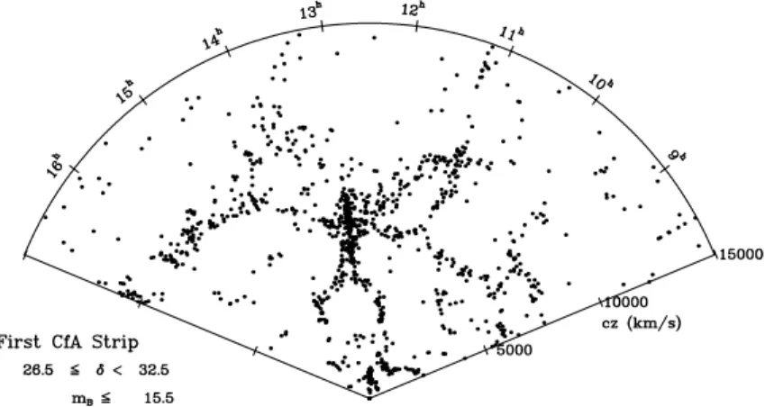
Figure 1.4: The second CfA survey. Image credit: The Smithsonian Astro-physical Observatory (de Lapparent et al.,1986).
The year 1986 marks an important step in the discovery and study of the large-scale structure of the Universe: Val´erie de Lapparent — a French Ph.D student doing her thesis in Cambridge (Massachusetts) under the supervision of Margaret Geller and John Huchra — published a redshift galaxy catalogue reaching m = 15.5 . The work was part of the CfA (Centre for Astrophysics) Redshift Survey, of which the first part had started in 1977. The map resulting from the second CfA spectroscopic survey is shown in Figure 1.4. The angle is much wider compared to previous surveys and confirms the idea that the distribution of galaxies is not random.
To illustrate the improvement that a few years had allowed in terms of survey’s area, we show in Figure 1.5 (Thompson and Gregory, 2011) a com-parison of the de Lapparent 1986 results with the earlier redshift survey from
Figure 1.5: Left panel: comparison between the second CfA survey (de
Lap-parent et al.,1986) and the Gregory and Thompson original plots (Thompson
and Gregory,2011); right panel: pushing a to di↵erent declination to see the
extent of the CfA Great Wall (Geller and Huchra, 1989) (8.5◦ < δ < 14.5◦,
while the de Lapparent was 26.5◦< δ < 32.5◦).
The slice from de Lapparent et al. (1986) can be seen as the passage to a new era, the era of large scale surveys. More than hints of structures could be clearly seen, enhancing certainty to the void-filament-sheet-cluster panorama of the large-scale structures. In the following years the map was further improved by completing the sampling in the area, which led to the detection of the CfA Great Wall, the largest sheet of galaxies ever detected until that time (see right plot of Figure 1.5, from Geller and Huchra (1989)). To complete this review of the history of the large-scale structure, I will cite and represent some of the most significative surveys of the following years, with no claim of completeness.
The joined CfA2 and SSRS2 (a magnitude-limited survey covering the re-gion around the south Galactic Pole) covered more that 30 % of the sky (da
Costa et al., 1994). The LCRS (Las Campanas Redshift Survey) is also an
important example, since it made use of an improvement in the technology to measure redshifts: fiber-fed multi-object spectrographs and wide-filed tele-scopes allowed to sample a five times larger volume (Shectman et al.,1996).
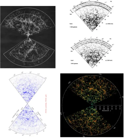
Jumping to most recent times, I cannot avoid mentioning the two largest redshift surveys completed until now: the 2dF Galaxy Redshift Survey and the Sloan Digital Sky Survey. All these most recent surveys are shown in Figure 1.6, allowing to observe the improvements from the first to the last.
Figure 1.6: From left to right, upper row: CfA-SSRS2 (da Costa et al.,1994) joint map, the LCRS (Shectman et al., 1996); lower row: the 2dF survey (last release, image credit 2dF Galaxy Redshift Survey) and the SDSS results (image credit: Sloan Digital Sky Survey).
After having presented the discovery of voids and of the Universe at large scales, the next Section briefly sums up the history of Cosmology.
1.2
An abridged history of Cosmology
Cosmology became a modern science when scientists started measuring the expansion of the Universe. Historically, this happened exactly after the aware-ness that there were other galaxies outside ours. While studying the story of
the large-scale structure, I jumped from Slipher’s work (in 1917) and the claim that the “nebulae” are in fact other galaxies to the first surveys of 1976.
Among the two, I skipped an important event that constitutes the first pillar of nowadays Cosmology: the discovery of the expansion of the Universe through the redshift-distance relation. The astronomer Edwin Hubble is the most known for the discovery of the expansion of the Universe. Nevertheless, as pointed out by Peacock (2013), Vesto Melvin Slipher had already mea-sured the expansion of the Universe before him and advanced the perceptive hypothesis that galaxies recede in all directions — his redshift measures were used by Hubble to reach the conclusion that the Universe is expanding. To the interested reader, I add details about his research in Appendix A.
Furthermore, the idea of expanding Universe had also been introduced before Hubble by another scientist, the Belgian abbey Georges Lemaˆıtre. In 1927, Lemaˆıtre had published “Un univers homog`ene de masse constance et de rayon croissant, rendant compte de la vitesse radiale des n´ebuleuses extra-galactiques” (Lemaˆıtre, 1927), in which — based on Slipher’s velocity mea-surements and on Hubble 1926’s distances (obtained using Leavitt’s relation) — Lemaˆıtre had in fact obtained the expansion rate of the Universe.
Livio(2011) discovered the reason for which Lemaˆıtre’s results were
unno-ticed by the scientific community and the Belgian astrophysicist did not have the deserved recognition; details about this interesting anecdote can be found in Appendix A.
After this brief reminder about the discovery of the expansion of the Uni-verse I introduce the pillars of modern Cosmology.
1.2.1
The pillars of Cosmology
In this Section I introduce the three pillars of Cosmology: the redshift-distance relation, the cosmological principle and the Friedmann-Lemaitre-Robertson-Walker metric.
The redshift-distance relation (known as the Hubble5 law) is one of the
basis of Cosmology. To illustrate the relation we remind the definition of red-shift. The observed shift of a galaxy’s spectrum through the identification of spectral absorption lines allows the calculation of the relative motion between source and observer on the basis of the Doppler e↵ect:
z = λo− λe λe
(1.1)
where λe is the emission wavelength and λo the observed wavelength. There
are three possible cases:
• If z < 0, the source is approaching the observer, this will result in a so-called blueshift (all spectral lines are displaced towards shorter wave-lengths).
• If z = 0, the source would not be moving either towards or away from the observer.
• If z > 0, the source is moving away from the observer. This will result in a redshift (all spectral lines are displaced towards longer wavelengths). A linear relationship can be established between a galaxy’s speed of recession v and the distance of the galaxy from the observer. This relationship has been confirmed by the Hubble Space Telescope. As previously discussed, most of the redshifts used in the 1929 paper from Edwin Hubble to obtain the relation were measured by Vesto Melvin Slipher, and a robust measurement was not reached until unexpectedly recent times (Peacock,2013). The law states:
v ' H0d = cz (1.2)
where c is the speed of light and H0 is the Hubble constant6. I anticipate that
H0 corresponds (as will be shown) to the value of H (the so-called Hubble
5We discussed in Appendix A the role of Edwin Hubble in the discovery, the perceptive
hypothesis by Slipher, the use of his data and the earlier discovery by Lemaˆıtre.
6For completeness, I show that equation 1.2 is a linear approximation that can be
ob-tained from the results in Section 1.2.3. Expanding a(to) in a power series we have:
parameter) in Friedmann’s equations at the time of observation. The mea-surement of the H0 is thus a measurement of the expansion of the Universe.
Pillar II: The cosmological principle:
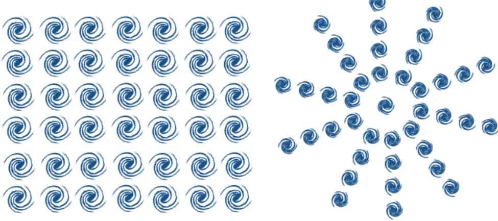
The second pillar of Cosmology is the cosmological principle which states isotropy (invariance in rotation) and homogeneity (invariance in transla-tion) of the Universe on large scales (larger than 100-200 Mpc). This leads to the absence of a privileged position or direction in the cosmos. To better understand the di↵erence between homogeneity and isotropy, we illustrate in Figure 1.7 two cases: a case of isotropy without homogeneity and a case of homogeneity without isotropy.
The application of the cosmological principle significantly limits the great variety of possible cosmological models. The cosmological principle is an as-sumption, since it has not been proved. On large scales however isotropy has been confirmed by many factors, such as:
• the distribution of clusters and superclusters of galaxies • the distribution of radiosources
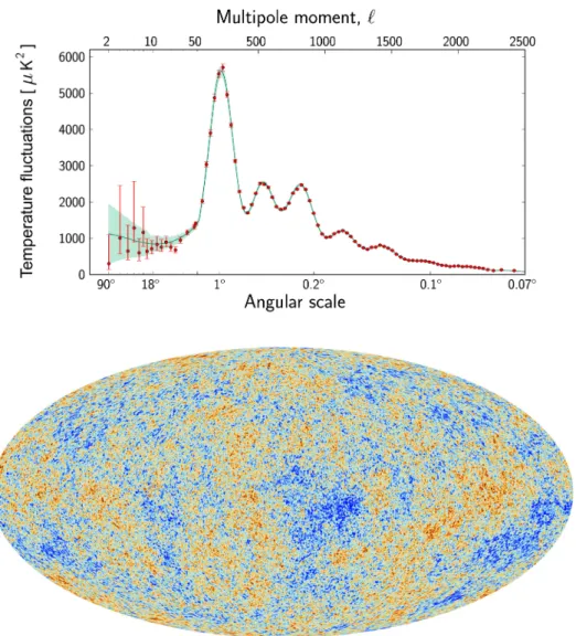
• the uniformity of the background radiation — particularly the Cos-mic Microwave Background radiation (CMB) which describes a strongly isotropic Universe at the time of the emission of the radiation, or the background X-radiation between 2 and 20 keV produced by unresolved sources up to distances of thousands of Mpc.
Although isotropy is not proved, by increasing the number of samples of cos-mological objects, isotropy rises. According to the Copernican principle, there is no reason to consider our position privileged, hence there must be isotropy in each point of the Universe. This strongly implies homogeneity.
considering equation 1.25 and multiplying on both sides by c, we obtain: cz= ˙a(te)
a(te)
c(to− te) + .... (1.4)
where it is possible to identify the Hubble law, with c(to− te) being the distance and ˙a(t
e)
a(te)
Figure 1.7: Left: illustration of homogeneity without isotropy, the image is invariant under translation, but would variate under rotation (the vertical and horizontal directions are preferred; if rotated of a certain angle, the two preferred directions would change, thus the image would change under rota-tion). Right: isotropy without homogeneity (translating the image would change it, but the image is invariant under rotation).
Since the Universe is expanding, it has reached the present low-density state from an initial hot and dense state, in a homogeneous and isotropic way. The model that predicts an initial hot and dense state is the Big Bang model. The homogeneity and isotropy of the Universe at large scales is a fun-damental assumption to work with cosmic voids, as explained in the next Chapter.
Pillar III: The Friedmann-Lemaitre-Robertson-Walker Metric
In the years between 1920 and 1930, four scientists worked independently on the model of an expanding Universe. Alexandre Friedmann was the first to look for exact solutions of the theory of General Relativity and published in 1922 a theory of expansion. Independently, in 1927, Georges Lemaˆıtre (as discussed in the previous section) wrote a paper establishing the expansion of the Universe. Furthermore, Howard Percy Robertson and Arthur Geo↵rey Walker autonomously developed a metric able to describe a homogeneous and isotropic Universe. Assuming the cosmological principle, it is thus possible to define the Friedmann-Lemaˆıtre-Robertson-Walker model for the expansion of the Universe. This model studies the Universe as a whole to understand its
evolution thanks to the assumption of homogeneity and isotropy that greatly simplifies the study.
To describe the Universe, we set a system of coordinates in space-time: three space coordinates (xα where α = 1, 2, 3) and a temporal coordinate
(t) which indicates the time, measured by an observer that is moving with the point. Generally, the geometrical properties of the coordinate system are determined by the metric tensor gµν. This approach allows to include the
e↵ects of gravity in the metric, which means that the motion of particles will be simply described as a motion in a distorted space-time. The interval ds between two events in space-time is defined by the most general expression:
ds2=X
µ,ν
gµνdxµdxν (1.5)
µ and ν have values from 0 to 3, where indices 1, 2 and 3 represent spatial coordinates and 0 is referred to the time-coordinate. When assuming the cos-mological principle, the metric gµν will take a simple form. To reach this form,
the coordinate system is chosen so that the space-time slices are homogeneous and isotropic at fixed t. This is equivalent to impose g0i = 0, such that the
slicing in time is orthogonal to the spatial part. The spatial grid is comov-ing7, so that an observer moving with it measures zero velocity for the cosmic
fluid (Lyth and Liddle, 2009): this guarantees isotropy also in an expanding Universe. Furthermore, we define
• The parameter t, called proper cosmological time (or cosmic time), is the time measured by an observer who sees the Universe evolving in a uniform expansion around him. To impose homogeneity, we set the proper8 time interval between slices as position independent, thus we
impose g00 = −1.
7The comoving distance is the distance between two points measured with a grid that
expands. If the Universe is expanding the physical distance between points will increase, but the comoving distance is defined as remaining constant. More details can be found in Section 1.2.3.
8Here the adjective proper defines the time measured by an observer that is at rest
• The scale factor a(t), which takes into account distances stretching over time, is normalized to a(H−1
0 ) = 1 at the present time. The scale factor
is extremely important in Cosmology, since it represents the relation be-tween the physical distance and the comoving distance bebe-tween objects. It is thus proportional to the distance between points and, if inserted into the metric for the spatial coordinates, it allows to preserve homo-geneity and isotropy during expansion. With the addition of this factor in the metric, the cosmological principle is preserved on a surface of constant t, but it is no longer a static Universe. We note that the scale factor can be related to redshift in an intuitive way: from 1.1, we can obtain:
z + 1 = λo λe
The expansion of the Universe can be thought as a proportional rela-tion between the observed and the emitted wavelengths, where the scale factor is the proportionality coefficient :
λe= a(te)λo
This is just a first intuitive description, a more complete derivation will be given in Section 1.2.3.
Taking into account all the above considerations, if the Universe is flat, the metric would be:
gµν = 0 B B B B @ −1 0 0 0 0 a2(t) 0 0 0 0 a2(t) 0 0 0 0 a2(t) 1 C C C C A
This is the Friedmann-Lemaˆıtre-Robertson-Walker metric. We made the as-sumption of a flat Universe. If you want to consider curvature, the interval ds can be written as:
ds2= −c2dt2+ a2(t)⇥dr2+ S2(r)d⌦2⇤
where the value of function Sk depends on the curvature of the Universe.
The spatial part of the metric is the spatial metric for a Universe with uni-form and constant curvature k of radius R0. The curvature constant k is
dimensionless and can take the values: −1 (a Universe with constant nega-tive curvature), 0 (a Universe that is spatially flat) and +1 (a Universe with constant positive curvature).
Depending on the values of the constant k, the function Sk(r) can take
di↵erent values: R sinh(r/R) if k = −1, r if k = 0 and R sin(r/R) if k = +1. In this way three di↵erent metrics can be obtained for a Universe in isotropic expansion or contraction:
• k = −1 −! The Universe is negatively curved and the metric is ds2= −c2dt2+ a2(t)⇥dr2+ R2sinh2(r/R)d⌦2⇤
• k = 0 −! The Universe is spatially flat and the metric is ds2= −c2dt2+ a2(t) [dr2+ r2d⌦2]
• k = +1 −! The spatial curvature is positive and the metric is ds2= −c2dt2+ a2(t)⇥dr2+ R2sin2(r/R)d⌦2⇤
Another form9 of the Friedmann-Lemaˆıtre-Robertson-Walker metric is:
ds2= −c2dt2+ a2(t) " dx2 1 − kx2 R2 0 + x2d⌦2 # (1.7)
where we have switched from radial coordinate r to x = Sk(r) (Ryden,
2003).
The Friedmann-Lemaˆıtre-Robertson-Walker model describes the expan-sion of the Universe under the hypothesis of the cosmological principle (namely isotropy and homogeneity). To correctly describe the Universe under the ap-proximation of the cosmological principle, the metric must be a solution of Einstein’s equation of General Relativity. The metric can indeed be related 9The difference between the two formulas is that when r is the radial coordinate, the
radial distances would be Euclidean, while angular distance are not. When x is the radial coordinate we have the contrary, so here we are only making a coordinate’s change.
to the energy and matter content of the Universe. This is the subject of the next section.
1.2.2
Friedmann equations
In order to explain the dynamic of the Universe, it is necessary to deter-mine the evolution of the scale factor. This can be done by establishing the relationship between the description of the metric of an homogeneous and isotropic space and the mass-energy contained in the Universe. This relation-ship is given by Einstein’s field equations which describe the dynamics of the Universe by determining the evolution of the scale factor a(t). If Gµν is the
Einstein tensor, Tµ
ν the stress-energy tensor (also called energy-momentum
tensor), Rµν the Ricci curvature tensor and R, the scalar curvature, defined
by R = gµνR
µν, then Einstein’s equations can be written:
Gµν ⌘ Rµν−
1
2Rgµν = 8πGTµν (1.8)
This set of ten equations describes the fundamental interaction of gravity as a result of space-time being curved by matter and energy. It gives the relationship between space-time geometry (represented by the metric and the Ricci tensor and scalar) and the energy and pressure at a point in space-time (related to the stress-energy tensor). Einstein’s equations will eventually require the calculation of the tensor components of the equation. First we consider the left side of 1.8. The Ricci tensor Rµν can be expressed through
the Christoffel symbols Γi
jk (Dodelson,2003) in the following way:
Rµν = Γαµν,α− Γαµα,ν+ Γβαα Γβµν − ΓαβνΓβµα (1.9)
where the commas indicate the derivatives with respect to the coordinate. The Christoffel symbols are linked to the metric gµν by the relationship:
Γµαβ = gµν 2 ∂gαν ∂xβ + ∂βν ∂xα − ∂gαβ ∂xν
expression of Γµαβ, we obtain the Christoffel symbols and, consequently, the
Ricci tensor and Ricci scalar. This allows the calculation of the Einstein tensor, which can then be written:
G00= 3 ✓ ˙a a ◆2 +3k a2 (1.10) G11= G22= G33= −2 ¨ a a− ✓ ˙a a ◆2 − k a2 (1.11) Gothers = 0 (1.12)
The stress-energy tensor in the right-hand side of equation 1.8 is extremely difficult to manage, indeed its form can be very complicated, especially in the case of inhomogeneity in the spatial energy distribution. A significant sim-plification can be obtained assuming a homogeneous Universe. In fact, in Cosmology, since many of the components of the Universe can be approxi-mately described as perfect fluids, the stress-energy tensor to be considered is the one representing a perfect fluid — a fluid that is isotropic, with negligible viscosity and heat conduction. Considering this particular case, Tµ
ν can be
written in the following way:
Tµ
ν = (ρ + P )UµUν+ P gµν
where ρ is the energy density of the fluid, P its pressure and Uµ its
four-velocity, with the normalization UµUν=1. According to Robertson-Walker’s
metric, the pressure P must be isotropic. Hence it can be written (with P and ρ only depending on time):
Tµ ν = 0 B B B B @ −ρ 0 0 0 0 P 0 0 0 0 P 0 0 0 0 P 1 C C C C A
Combining this expression of the stress-energy tensor with the Robertson-Walker metric 1.6 we can obtain Friedmann’s equation (Friedmann,1922;
Ryden,2003): H2=✓ ˙a a ◆2 = 8πG 3c2 X i ρi− kc2 R2 0a2 (1.13)
where R0 is the radius of curvature of the Universe and the summation is
extended to all kinds of energy present in the Universe (which are weighted in di↵erent ways by the evolution of the scale factor with time). We have used H = ( ˙a/a), anticipating a result that will be shown in Section 1.2.3.
This equation is valid for any Universe which follows the Friedmann-Lemaˆıtre-Robertson-Walker metric and whose expansion or contraction is ruled by General Relativity. In fact a Universe that follows Friedmann’s equa-tion is an isotropic and homogeneous soluequa-tion of Einstein’s equaequa-tions.
In a flat Universe (k=0), Friedmann’s equation becomes a very simple expression. For any given value of the Hubble parameter, we can define the critical energy density as:
ρc =
3H2c2
8πG (1.14)
If the energy density is greater than ρc, the Universe is positively curved
(k = +1). If the energy density is smaller than ρc, the Universe has a negative
curvature (k = −1). We can then introduce the density parameter as the ratio of the total energy density and the critical energy density:
⌦tot(t) =
P
iρi
ρc
(1.15)
The density parameter binds the total energy density to the geometry of the Universe: ⌦tot 8 > < > : > 1 −! k = +1 = 1 −! k = 0 < 1 −! k = −1 Friedmann’s equation can then be written:
1 − ⌦tot(t) = −
kc2
R2
0(a(t))2(H(t))2
We can define the curvature component: ⌦k(t) = − kc2 R2 0(a(t))2(H(t))2 (1.16)
Considering the present time, we have
⌦k0= 1 − ⌦0= −
kc2
R2 0H02
,
where it can be seen that the curvature of the Universe depends on the total energy density.
Knowing ⌦0, the sign of the curvature k can be found.
Friedmann’s equation has got two variables: a and ρ. Another relationship is therefore needed that includes both of them as functions of time. The principle of energy conservation will allow us to find this relationship. It is expressed by the first law of thermodynamics:
dQ = dE + PdV
We consider a sphere of comoving radius rswhich expands as a result of the
expansion of the Universe. If the Universe is perfectly homogeneous, for each comoving volume filled with any fluid, the expansion will be adiabatic. This means that the net heat flux dQ will be zero. The first law of thermodynamics can be applied to any fluid contained in a comoving volume; because of the cosmological principle, for each volume dV, dQ should be zero. The first law of thermodynamics can then be written: ˙E + P ˙V = 0. But we also have: E(t) = V (t)ρ(t), hence we obtain the flux equation
˙ρ + 3˙a
a(ρ + P ) = 0 (1.17)
Combining this equation with Friedmann’s equation we can derive the ac-celeration equation(Ryden,2003) which gives the variation of acceleration with time: ¨ a a = − 4πG 3c2 X i (ρi+ 3Pi) (1.18)
For positive pressure, if the energy density is greater than zero this equa-tion gives a negative acceleraequa-tion, which means that the relative speed of two points decreases. If we consider as an additional variable P (the pressure of the matter that fills the Universe), we end up with three equations with three unknowns. However, these three equations are not independent, since the acceleration equation is obtained from Friedmann’s equation.
We shall therefore introduce an equation of state to combine the pressure and the energy density of the matter that fills the Universe. Since the Universe is very diluted, it can be described as a perfect fluid. Under this assumption, the pressure and the energy density are bound through the equation of state parameter ω, which varies depending on the component being considered.
The relationship is: P = ωρ. Considering the relation for each component is a way of describing how the content of the Universe a↵ects its evolution. This will be briefly reviewed in Section 1.3.1.
1.2.3
Distances
In the last Section I introduced the standard cosmological model and its three pillars: the redshift-velocity relation, the cosmological principle and the Friedmann-Lemaˆıtre-Roberston-Walker metric. Finally I described Fried-mann’s equations.
Another important point in Cosmology is the definition of distances. In the measurement of distances, there is a practical and conceptual issue: how can we define the distance between two points in an expanding Universe? The truth is that many di↵erent kinds of distances can be defined.
I will review the definitions and physical meanings of the following dis-tances: comoving distance (line of sight and comoving), proper distance, Hubble distance, angular diameter distance and luminosity distance (an useful reference isHogg (1999)).
Line of sight comoving distance
The Universe is expanding, distances between objects are a↵ected by the expansion. It is then useful to consider a measure of distance that remains
una↵ected by the expansion: the comoving distance. As anticipated in Section 1.2.1, one can consider a grid that expands with the Universe. If we define points in such comoving grid, we are using a comoving coordinate system. The distance defined in this system is the comoving distance.
The comoving distance to an object at redshift z = a(t)−1− 1 is:
χ(a) = Z t0
t(a)
cdt0
a(t0) (1.19)
This distance is between us and another object (as given by the formula), or between objects at di↵erent redshift (and thus at a di↵erent time).
Transverse comoving distance
On the contrary, the transverse comoving distance is between objects at the same z. It is equivalent to the proper motion distance (Hogg,1999) dM (which
is given by the ratio of the actual transverse velocity to its proper motion, in radians per unit time (Weinberg,1972)). If the Universe is flat, the transverse comoving distance is equal to the line of sight comoving distance10 χ.
Proper distance
I now consider the proper distance. In an expanding Universe, the distance between two points increases with time. I thus define the proper distance dp(t)
as the length of the spatial geodesic11 between two points at a fixed value of
the scale factor, that is at constant cosmic time.
This distance thus changes over time due to the expansion of the Universe. More precisely, as defined by (Davis and Lineweaver, 2004), at a particular time t it is the distance that we can measure along the line of sight using a series of infinitesimal comoving rulers. An observer is placed near each ruler 10This explains why sometimes we only generally refer to the comoving distance without
further specification.
11In fact, light travels along geodesics. These are curves with geodesic curvature equal
to zero, where the geodesic curvature is a property of curves which reflects the deviance of the curve from following the shortest arc length distance along each infinitesimal segment of its length. In simplest terms, a geodesic is a curve that locally describes the shortest trajectory between points in a particular space. In the case of photons it must be ds = 0.
and measures its distance to the nearest observer; the proper distance is the sum of all distances. One would thus need synchronized comoving observers to measure proper distance.
To give a simplified expression of dp(t), we consider a fixed time (dt = 0);
from equation 1.6, since the angles are constant over the spatial geodetic (d⌦=0), we obtain ds = a(t)dr (considering a flat Universe). The proper distance can be obtained integrating over the comoving radial coordinate r:
dp(t) = a(t)
Z r
0
dr = a(t)r (1.20)
However the proper distance can also be defined in a di↵erent way. Con-sidering Friedmann’s equation in the case of a Universe composed of matter, radiation and a cosmological constant, we have:
H2 H2 0 = ⌦r,0 a4 + ⌦m,0 a3 + ⌦Λ,0+ 1 − ⌦0 a2
By considering the definition of the Hubble parameter H = ˙a(t)/a and inte-grating, it is possible to obtain (Ryden,2003):
dp(to) = c H0 Z 1 a(te) da a(t0)2(⌦ r,0a−4+ ⌦m,0a−3+ ⌦Λ,0+ ⌦k,0a−2)1/2 (1.21)
This distance is defined at a particular moment of time and, as the Universe is expanding, it is not measurable.
The definition of proper distance allows us to obtain a relationship between the scale factor and Hubble’s parameter. Using the proper distance we can reformulate the redshift-distance relation:
vp(t) = ˙dp(t) = ˙a(t)r =
˙a(t)
a(t)dp(t) = H(t)dp(t)
which gives the relationship between the scale factor and Hubble’s parameter:
H = 1 a da dt = ˙a a (1.22)
This definition is extremely important in Cosmology, this is the reason why we formulate it here. If we evaluate it now, it gives us H0, the Hubble’s constant.
Hubble distance
We define the Hubble distance:
dH(t0) =
c H0
(1.23)
as the critical distance such that two points at a distance greater than dH(t0)
will have vp> c.
The Hubble distance is not a distance that can be defined between any two objects, since it is the distance between us and the objects with super-luminar speed. There is some confusion related to these objects in an expanding Universe (Davis and Lineweaver, 2004): the super-luminous speed of objects refers to their relative motion inside an expanding Universe and therefore does not violate the law limiting the speed of massive objects at the speed of light. The redshift-distance relation thus gives super-luminar speed for objects. This is perfectly allowed in the framework of General Relativity, since faster than light motion occurs outside the observer’s inertial frame. Galaxies receding from us super-luminally are at rest with respect to the cosmological frame
(Davis and Lineweaver,2004).
With H0 obtained from the Planck mission (Planck Collaboration,2013),
and using the approximate redshift-distance relation, we have dH(t0) = 4455
Mpc. Galaxies farther than this distance are moving away from us at super-luminar speeds, along with the photons they emit.
We use the given definitions to find the relationship between the redshift z of a distant object and the scale factor at the moment of the emission of the light, a(te). In the case of a distant galaxy, the light emitted at time te
is observed at time to. During its path the light travels along a null geodesic,
with ds = 0 and with constant angles θ and ϕ. Hence, along the null geodesic, we have: c2dt2 = a(t)2dr2 and so ca−1(t)dt = dr. Integrating between t
to and considering only one wavelength λe, we have c Z to te dt a(t) = Z r 0 dr = r
The forthcoming wavelength, emitted at the time te+λce, will be observed at
time to+ λco and will get us to a similar integral with the same second term
r, therefore: Z to te dt a(t) = Z to+λoc te+λec dt a(t)
Subtracting the integral between te+ λce and to from each side of this latter
equation, we have: Z to te dt a(t)− Z to te+λec dt a(t) = Z to+λoc te+λec dt a(t)− Z to te+λec dt a(t) Z te+λec te dt a(t) = Z to+λoc to dt a(t)
We can compare the time between the emission and observation for the two wave crests with the age of the Universe. We obtain a rough approximation of the age of the Universe t0 using Hubble’s law:
t0 = r v = r rH0 = H−1 0 ' (14.0 ± 1.4)Gyrs
Since t0>> λ/c, we can assume that between two wave crests (regardless
of whether we are considering emission or observation) the Universe has not expanded by a significant amount. Hence we can say that a(t) has remained constant during that time. Thus the integrals give:
λe
a(te)
= λo a(to)
(1.24)
and finally, since the redshift is defined as
z = λo− λe λ
we obtain: 1 + z = a(to) a(te) = 1 a(te) (1.25)
where the equation has been normalized with a(to) = ao = 1. This equation
gives the relationship between the redshift z of a distant object and the scale factor at the moment of the emission of the light a(te). It shows that the
redshift for a distant object depends only on the ratio of the scale factors at the times of emission and observation and not on the way in which the light passed between a(te) and a(to).
The distances we have introduced so far are distances that we cannot measure easily. A more directly measurable distance will be presented in the next section.
Angular diameter distance
A direct way to measure distances in Astronomy is through the angle12
sub-tended by an object of known physical lenght l (Dodelson, 2003), assuming for simplicity that this object is disposed perpendicularly to the view line. We obtain the angular diameter distance:
dA⌘
l?
δθ (1.26)
The object size l? and its proper diameter r are related through l?= a(te)rδθ
(this can be shown using FLRW at a fixed time, in a flat Universe, con-sidering the distance ds between the two sides of the object). Therefore, δθ = l?/(a(te)r) (Peebles, 1993;Weinberg,1972).
Thus, substituting δθ in 1.26, the angular diameter distance can be written as: dA= l?a(te)r l? = a(te)r = a(t0) 1 + zr = r 1 + z = DM 1 + z (1.27)
where DM is the transverse comoving distance, equal to the line-of-sight
comoving distance χ if the Universe is flat. The generalisation for a non-flat 12Assuming a small angle.
Universe gives:
dA=
Sk(r)
1 + z
The angular diameter distance has a maximum for a precise value of z, denoted by zmax. In a model with ⌦m,0 = 0.3 and ⌦Λ,0 = 0.7, zmax becomes
1.6, which corresponds to the angular distance dA,max = 1800 Mpc. This is
intuitively strange, because objects at redshift higher than zmax will appear
to have smaller dA, they will have a large angular size. We can explain this
considering that when the light of the object was emitted, the Universe was much smaller (since it was in the past and the Universe is expanding), the object thus occupied a larger fraction of the Universe’s size.
We will discuss this more extensively in Section 2.1. Before concluding the description of the angular diameter distance, we point out that some confusion might arise for the definitions used of the angular distance: some references call dAthe angular diameter distance, while others use the same symbol for the
comoving angular diameter distance dAcom (such as Weinberg et al. (2012)).
To avoid confusion, we use di↵erent symbols and note that:
dAcom= adA=
dA
1 + z (1.28)
The luminosity distance
Another intuitive way to measure distance is through the use of luminosity. If we have an object of known luminosity, it is possible to establish at which distance it is by the fading of its brightness. Measuring the energy flux f received on Earth and knowing the intrinsic luminosity of the object we can define a function called luminosity distance:
dL= ✓ L 4πf ◆1/2 (1.29)
This function would correspond to the proper distance if the Universe were static and Euclidean. In reality, the expansion of the Universe results in a diminution of the photon energy flux by a factor (1 + z)−2. Let us consider
is a(te). This photon would be observed now, when a(t) = a(to) = 1. Then,
because of wavelength stretching, E0 = Ee/(1 + z).
Moreover we can consider the case of two photons emitted in the same direction and separated by a temporal gap δte. At the beginning, their proper
distance is cδte and at time to, it will be cδte(1 + z). This means that the
time interval between the emission of the two photons increases, as is shown by the equation:
δto= δte(1 + z)
Therefore the frequency of the detection decreases.
Finally, in an expanding Universe governed by the Friedmann-Lemaˆıtre-Robertson-Walker model, the relationship between flux and luminosity is:
f = L
4πSk(r)2(1 + z)2
Hence the luminosity distance is dL= Sk(r)(1 + z). The luminosity distance
of an object with redshift z depends both on the geometry of the Universe and on its dynamics.
The latest observational data13 seem to indicate a flat geometry for our
Universe. We recall that the function Sk(r) takes the following values:
Sk(r) 8 > < > : sin(r) () k = +1 r () k = 0 sinh(r) () k = −1
Since k = 0, the luminosity distance can then be written (Ryden,2003):
dL= r(1 + z) = dp(t0)(1 + z) (1.30)
In a non-flat Universe, we have:
dL= Sk(r)(1 + z) = dp(t0)(1 + z) (1.31)
13BOOMERANG (de Bernardis et al.,2000) and the Planck satellite (Planck
Moreover, when z << 1, we have: dL' c H0 z ✓ 1 +1 − q0 2 z ◆ (1.32)
where we have used the deceleration parameter14(Peacock,1999).
Comparing distances
Using the definitions of dL and dA (equations 1.30 and 1.27 respectively), we
obtain the following relation (Weinberg,1972)15
dL= (1 + z)2dA
In the case of a flat Universe and assuming z −! 0 (i. e. at low redshift), the following relations between distances can be established. As a start, the luminosity distance is a good approximation of the proper distance at the present time. Indeed, dp(t0) ' dL ' (c/H0)z.
Moreover, as k = 0, dA(1 + z) = dL/(1 + z) = dp(to), then
dA =
dp(to)
1 + z = dp(te)
Furthermore, if z << 1, the angular diameter distance can be approximated 14The deceleration parameter is defined as
q0= −✓ ¨a ˙a2 ◆ t=t0 = − ✓ ¨ a aH2 ◆ t=t0
The deceleration parameter is adimensional and its value is negative if the expansion of the Universe is accelerating. It will be positive if the expansion is decelerating. It was called the “deceleration parameter” because it was introduced at a time when the Universe was believed to be dominated by matter and therefore undergoing a decelerated expansion. The deceleration parameter allows to approximate the scale factor:
a(t) ' a(t0) + da dt 6 6 6 6t =t0 (t − t0) + 1 2 d2a dt2 6 6 6 6t =t0 (t − t0)2= 1 + H0(t − t0) − 1 2q0H 2 0(t − t0)2 (1.33) 15Note that this relation, written in terms of the comoving angular diameter distance,
using the deceleration parameter: dA ' c H0z(1 − 3 + q0 2 z) Thus as z −! 0 we have: dA' dL' dp(t0) ' c H0 z (1.34)
This can be understood thinking that at small distances the Universe seems Euclidean, even though the space-time is curved. Having introduced the ba-sis of Cosmology and its history, we now describe the most recent model of Cosmology.
1.3
Recent developments in Cosmology
The Cosmological Constant
In 1917, two years after the publication in Annalen Der Physik of the article on General Relativity, Einstein considered applying his equations to the Universe as a whole. Since he had no experimental evidence about the expansion of the Universe and was unaware of the existence of the cosmic background radiation, Einstein was persuaded that the Universe was static. He imagined that much of the radiation in the Universe was provided by stars and that the main contribution to the energy density of the Universe came from non-relativistic matter. He therefore considered the approximation of a Universe without pressure (that is, more precisely, with positive energy density and negligible pressure).
However, he realised that a Universe that contained nothing but matter could not be static, so he inserted a factor ⇤ in his equations, which he called the cosmological constant, so that the equations would describe a static Universe filled with matter that was in accordance with his particular beliefs.
With the introduction of ⇤, the Friedmann equation becomes: ✓ ˙a a ◆2 = 8πG 3c2 ρ − kc2 R2 0a2 +⇤ 3
the fluid equation does not change and the acceleration equation becomes:
¨ a a = − 4πG 3c2 (ρ + 3P ) + ⇤ 3
It must be noted that adding ⇤ to the Friedmann equation is equivalent to adding to the Universe a component with negative pressure:
PΛ = −ρΛ = −
c2
8πG⇤
In order to have a static Universe, both ˙a and ¨a must be zero. Such solu-tions exist for a closed Universe, k = 1, and positive cosmological constant. Even then, the resulting model proposed by Einstein was unstable because the attractive force of ρ was in unstable equilibrium with the repulsive force of ⇤. When the expansion of the Universe was discovered, Einstein, faced with experimental evidence, abandoned both the idea of a cosmological constant and his belief in a static Universe, calling the introduction of ⇤ his “biggest blunder”. After having been reconsidered many other times, when the current value for H0 was too small compared to the age of observed objects, the
cos-mological constant has finally been reintroduced on the basis of observational data that indicate that the expansion of the Universe is, indeed, accelerating.
2011: a Cosmology Nobel Prize
The observational data that led to reconsidering the cosmological constant16
were obtained from a phenomenon exhibited by stars with very particular properties that can be used for the establishment of their distance, Type Ia supernovae (explosions of stars in binary systems that can be used as markers of the cosmic expansion). More details are given in Section 2.1.
16The case for observations favouring a cosmological model with large cosmological