The development of convective instability during SESAME, 1979

by

Frank Parker Colby, Jr. B.S., University of Michigan

(1976)

M.S., Massa-chusetts Institute of Technology (1979)

Submitted to the Department of Meteorology and Physical Oceanography

in Partial Fulfillment of the Requirements of the Degree of

DOCTORATE OF PHILOSOPHY at the

MASSACHUSETTS INSTITUTE OF TECHNOLOGY February, 1983

c Mas-s-a=chuset.ts Institute of Technology, 1983

Signature of Aut.ho-r

Certified by

Accepted by

Department of Meteorology and Physical Oceanography. 6 January 1983

Frede Snders, Thesis Supervisor

Ronald G. Prinn, Chairman, Departmental Committee on Graduate Students

Undgreh

MAR 22 1983

DEVELOPMENT OF CONVECTIVE INSTABILITY DURING SESAME, 1979 by

FRANK PARKER COLBY, JR. Submitted to the Department of Meteorology and Physical Oceanography

on 25 January 1979 in partial fulfillment of the requirements for the Degree of Doctorate in Philosophy

ABSTRACT

Convection in t-he Central United States is assumed to require the presence of convective instability and a triggering

mechanism to release the instability. Often, a stable layer

caps the PBL, preventing or delaying the release of convective

instability. The development of both convective instability and convective inhibition (from the stable layer) is studied with data from three cases from the SESAME field project of

1979. The cases are: 19-20 April, 9-10 May. 6-7 June. The data are analyzed and both convective instability and inhibition are quantified.

A one-dimensional thermodynamic model which includes

radiation, a surface energy balance, and routines to predict soil and boundary layer characteristics is used as a tool to understand the imp-ortant physical factors involved in the development o-f convective instability and inhibition.

The results show that some convective instability was present before dawn in all three cases. The boundary layer heating during the day added to the initial instability. Soil

moisture, clouds, and changes in atmospheric structure above the PBL were all important Pactors controlling the PBL

evolution.

The modelled convective instability grew during the day as a result oF the boundary layer heating. Increased soil moisture

sometimes exerted a positive influence on the growth of

instability, but in other cases limited the growth by keeping the PBL from heating and deepening. Clouds gene-rally reduced. the convective instability growth, but in the June case,

clouds had the opposite effect. The influence of changes above the PBL was stronger on the reduction o- convective inhibition than on the growtn of convective instability. For these cases, the inPluence on the growth of convective instability from changes above the PBL was stronger than the presence of clouds or the increase of soil moisture, but all o these Factors were able to modify the development of convective instability and inhibition.

The results of the modelling and the observations show that the convection occurred where and when the inhibition was

reduced to low values. The convection began when the available forcing was sufficient to overcome the remaining inhibition. Therefore, the forecasting of convective outbreaks requires the ability to measure and predict the convective inhibition within the larger region of cbnvective instability.

Thesis Supervisor: Dr. Frederick Sanders Title: Professor of Meteorology

TABLE OF CONTENTS ITEM PAGE Abstract ... Table of Contents ... List of Figures ... L ist of Tables ... ... ... 1. Introduc-tion ... 2. Model 2.1 Introduction ... 2.2 Atmospheric Structure... 2.3 Conceptual Model Run .... 2.4 Radiation ...

A. Incident Radiation . B. IR Emission ... 2.5 Radiation Data Comparison 2.6 Surface Energy Balance .. A. Sensible and Latent

B. Soil Heat Flux ... 2.7 Ground Variables ... 2. - Boundary Layer Variables 2.9 PBL Temperature and Moist 2.10 Initialization Procedure 2.11 Sensitivity Tests ... A. TBAR Test ... B. VS Test ... C. WMAX and GWB Test .. D. GWO Test ... 2.12 Comparison Runs ... 2.13 Model Comparison Summary Tables for Chapter 2 ... Figures for Chapter 2 ...

es ...• ... • Hea ure ... • ... . .. ° •

3. Case St-udy I: 19 April 3.1 Introduction ... 3.2 Synoptic Analysis . 3.3 Mesoscale Analysis 3.4. Soundings ... 3.5 Hybrid Modelling .. 3.6 Summary ... lables for Chapter 3 ... Figures for Chapter 3

14 15 27 28 29 30 30 32 34 36 36 38 38 40 42 42 44 46 46 48 50 51 54 57 61 74 74 75 76 80 98 104 111

4. Case Study II: 9 May 4. 1 Introduction ... 4.2 Synoptic Analisis. ... 4. 3 Mesoscale Analysis ... 4.4 Soundings ... 4.5 21 GMT Modelling ... ... 4. 6 Summary for 21 GMT Modelling

4. 7 23 GMT Modelling ... 4.8 Summary for 23 GMT Modelling Tables for Chapter 4 ... Figures for Chapter 4 ... 5. Case Study III: 6 June

5. 1 Introduction ... 5.2 Synoptic Analysis 5. 3 Mesoscale Analysis 5.4 Soundings ... 5. 5 Hybrid Modelling .. 5. 6 Summary ... Tables for Chapter 5 ... Figures for Chapter 5 6. Conclusions ... .. Appendices 7. 1 Derivation 7.2 Derivation 7.3 Derivation 7.4 Derivation 7.5 Derivation of Radiation Parameterization ... of Ekman Layer Similarity Equations of Soil Heat Flux Parameterization of Ground Variable Equations .... of Inversion Equations ... References ... ... ... Acknowledgements ... ... 290 295 298 300 304 305 309 145 145 146 151 155 165 168 172 177 183 225 225 226 230 237 243 247 250 280

LIST OF FIGURES

2. 1 Schematic diagram of model atmosphere. 61

Q.2 .Comparison of model net radiation and soil fluxes with observations and modelling by Wetzei (1978) for O'Neill

day number 2. 62

2.3 Comparison of model IR cooling rates with calculations

of Rogers and Walshaw (1966). 62

2. 4 Comparison of model IR cooling rates with calculations of Brooks. (1950), Elsasser (1942), and ECMWF (1979). 63 2.5 Model IR cooling rates only for cloud layer of variable

coverages. 64

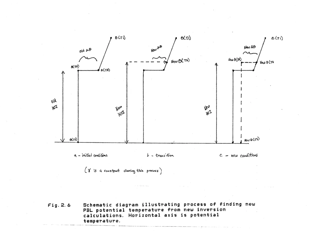
2.6 Schematic diagram illustrating process of finding new PBL potential temperature from new inversion

calculations. 65

2. 7 Schematic diagram showing process of initialization of

A~ from initial sounding. 66

2.8 Sounding plotted on a pseudoadiabatic diagram from

O'Neill, Nebraska at 1200 GMT. 67

2. 9 Time variation of pressure level of PBL top for standard

model run. 67

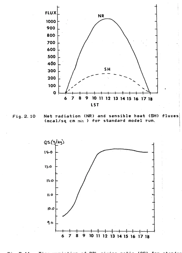
2. 10 Net radiation and sensible heat fluxes for standard

model run. 68

2. 11 Time variation of PBL mixing ratio for standard model

run. 68

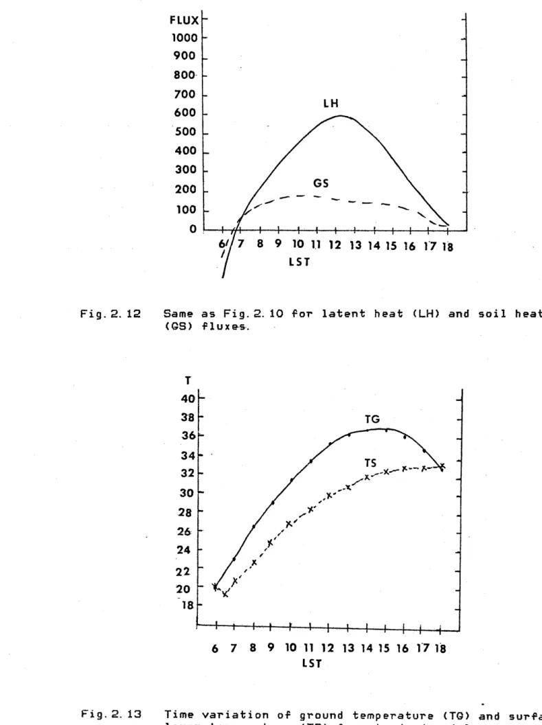
2. 12 Latent heat and soil heat fluxes for standard model

run. 69

2. 13 Time variation of ground temperature and surface layer

temperature for standard model run. 69

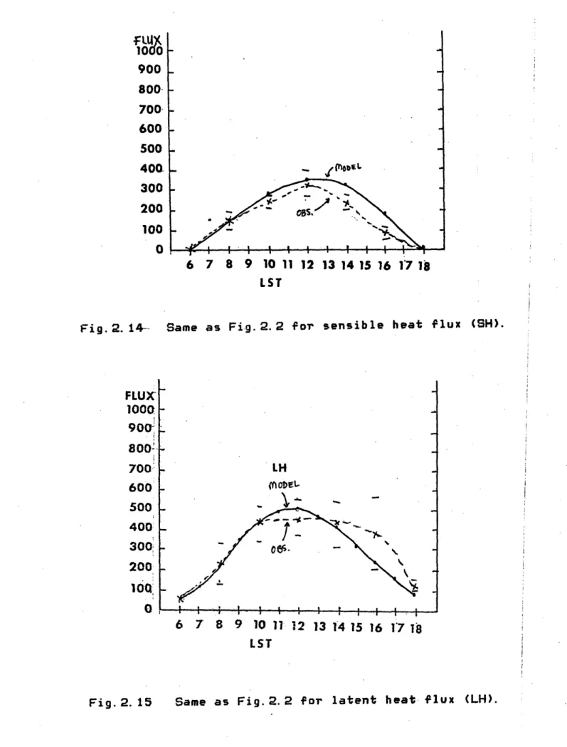
2.14 Comparison of model sensible heat flux with

observations and modelling by Wetzel (1978) for O'Neill

day number 2. 70

2. 15 Comparison of model latent heat flux with observations

for O'Neill day number 2. 70

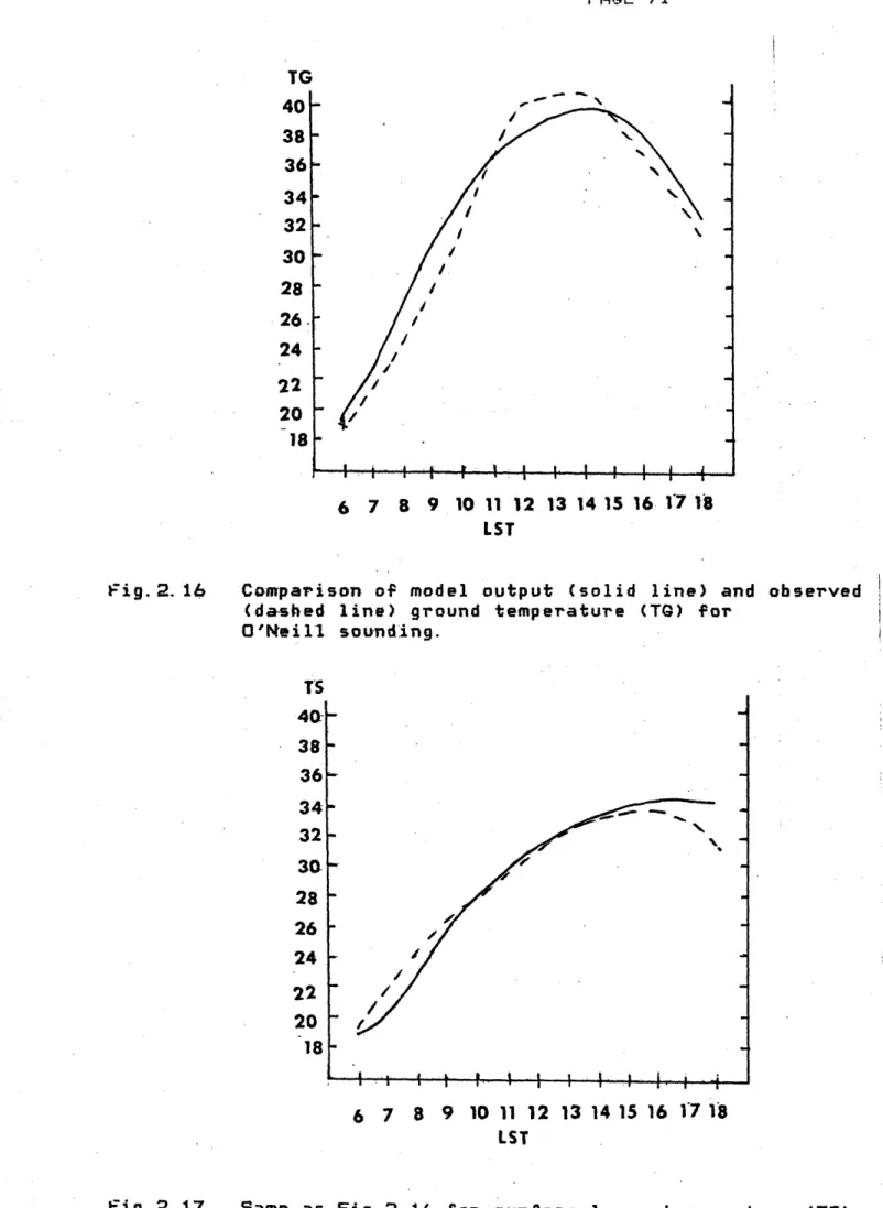
2.16 Comparison of model output and observed ground

2. 17 Comparison of.model output and observed surface layer

temperature for O'Neill sounding. 71

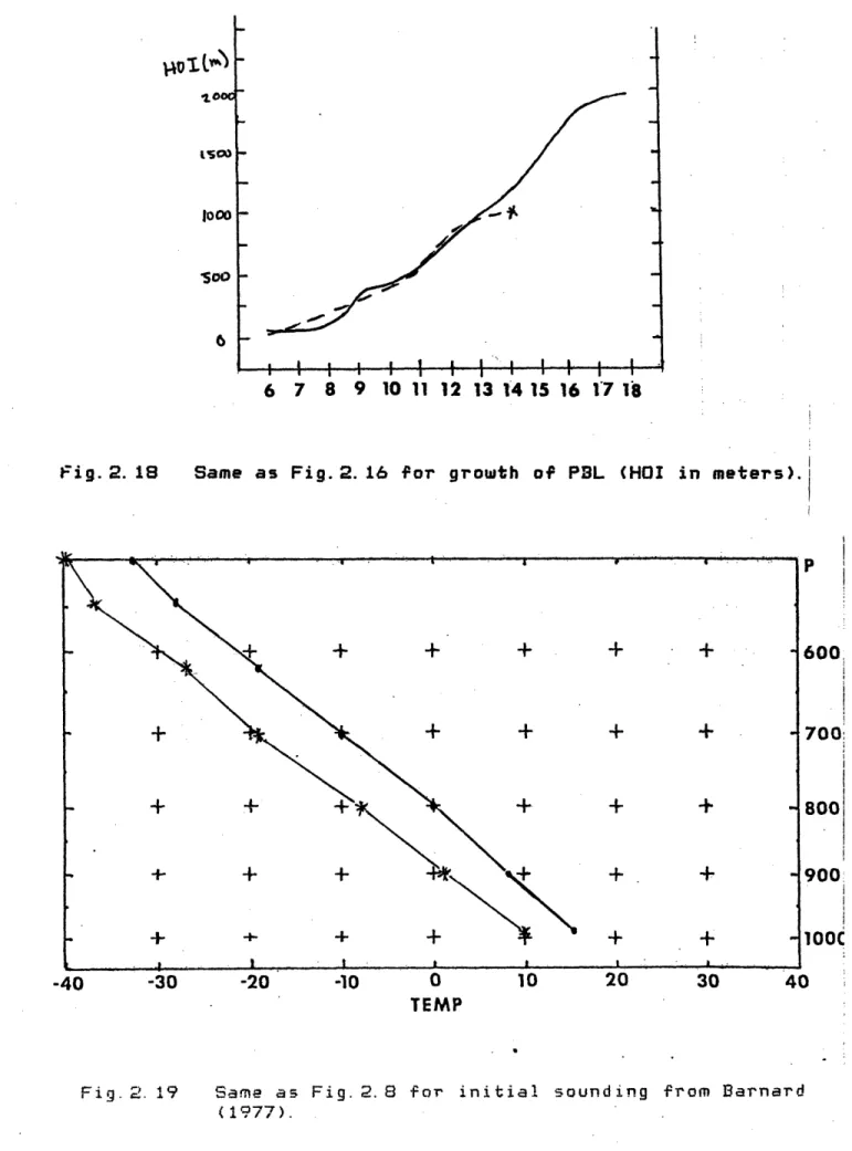
2. 18 Comparison of model output and observed growth of PBL

for O'Neill sounding. 72

2. 19 Sounding plotted on a pseudoadiabatic diagram from,

initial sounding from Barnard (1977). 72

2.20 Comparison of Barnard's (1977) model output with

present model output for PBL moisture at 0700 LST. 73 2.21 Comparison of Barnard's (1977) model output with

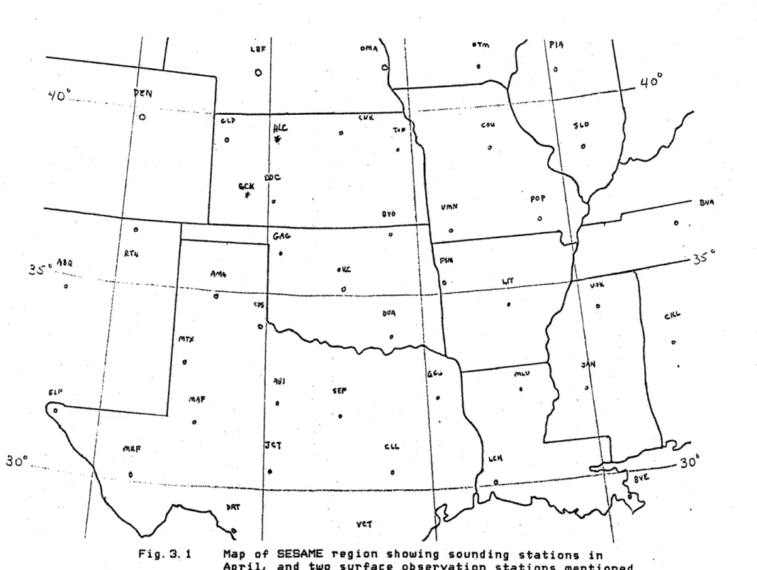
present model output for PBL moisture at 1000 LST. 73 3. 1 Map of SESAME region showing sounding stations in April, and two surface observation stations mentioned later in

the text. 111

3.2 500 mb analysis for 12 GMT, 19 April. 112

3.3 500 mb analysis-for 00 GMT, 20 April. 113

3.4 Synoptic-scale analysis for 12 GMT, 19 April. 114 3.5 Synoptic-scale analysis for 00 GMT, 20 April. 115 3.6 Photo.of low-elevation angle radar screen display at

Garden City, Kansas, 2102 GMT, 19 April. 116 3.7 Photo of low-elevation angle radar screen display at

Garden City, Kansas, 2122 GMT, 19 April. 116 3.8 Photo of low-elevation angle radar screen display at

Garden City, Kansas, 2140 GMT, 19 April. 117 3.9 Photo of low-elevation angle radar screen display at

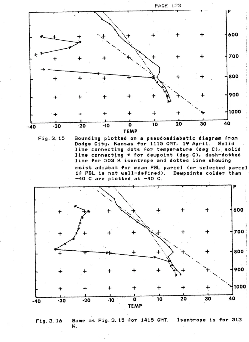
Garden City, Kansas, 2200 GMT, 19 April. 117 3. 10 Mesoscale surface analysis for 12 GMT, 19 April. 118 3. 11 Mesoscale surface analysis for 16 GMT, 19 April. 119 3. 12 Visible satellite photo for 1601 OMT, 19 April. 120 3. 13 Mesoscale surface analysis for 21 GMT, 19 April. 121 3. 14 Mesoscale surface analysis for 22 GMT, 19 April. 122 3. 15 Sounding plotted on a pseudoadiabatic diagram from

Dodge City, Kansas for 1115 GMI, 19 April. 123 3. 16 Sounding plotted on a pseudoadiabatic diagram from

Dodge City, Kansas for 1415 GMT, 19 April. 123 3. 17 Sounding plotted on a pseudoadiabatic diagram from

Dodge City, Kansas for 1715 GMT, 19 April. 124 3. 18 Sounding plotted on a pseudoadiabatic diagram from

Dodge City, Kansas for 2015 GMT, 19 April. 124 3. 19 Sounding plotted on a pseudoadiabatic diagram from

Goodland, Kansas for 1124 GMT, 19 April. 125 3. 20 _{Sounding plotted on a pseudoadiabatic diagram from}

Goodlandi, Kansas for 2007 GMT, 19 April. 125 3. 21 _{Sounding plotted on a pseudoadiabatic diagram from}

model output for 20 GMT from GLD initial sounding. 126 3. 22 Sounding plotted on a pseudoadiabatic diagram from

Concordia, Kansas for 1108 GMT, 19 April. 126 3. 23 _{Sounding plotted om a pseudoadiabatic diagram from}

Concordia, Kansas for 2008 GMT, 19 April. 127 3. 24 Sounding plotted on a pseudoadiabatic diagram from

model output for 20 GMT from CNK initial sounding. 127 3. 25 _{Change in surface potential temperature and dewpoint 12}

GMT to 22 GMT, 19 April. ₁₂₈

3.26 Sounding plotted on a pseudoadiabatic diagram for

initial h.gbrid sounding at 11 GMT, 19 April. 129 3.27 Map of rainfall in Kansas on 18 April. 130 3.28 Time variation of model output for HYB sounding, 19

April, 50-50 soil parameters with no extra factors. 131 3. 29 _{Time variation of model output for HYB sounding, 19}

April, 50-50 soil parameters with morning clouds

imposed. 132

3. 30 _{Time variation of model output For CNK sounding, 19} April, 70-80 soil parameters with no clouds. 133 3. 31 Time variation of model output for CNK sounding, 19

April, 70-80 soil parameters with "all day" clouds. 134 3. 32 Portion of sounding data from Dodge Citu, Kansas

plotted on a pseudoadiabatic diagram for ii GMT and 14

GMT, 19 April. 135

3. 33 Time -variation of model output for HYB sounding, 19 April, 50-50 soil parameters with inversion changes

imposed. 136 3.34 Time variation of model output for. HYB sounding, 19

April, 50-50. soil parameters with DDC and inversion

changes imposed. 13"7

3.35- Time vari'ation oF model output for HYB sounding, 19 April, 50-50 soil parameters with GLD and inversion

changes imposed. 138

3.36 Sounding plotted on a pseudoadiabatic diagram for model output for 21 GMT from HYB initial sounding with GLD

and inversion changes imposed 139

3.37 Time variation of model output for HYB sounding, 19 April, 50-50 soil parameters with DDC and inversion

changes and morning clouds imposed. .140

3.38 Time variation of model output for HYB sounding, 19 April, 50-50 soil parameters with GLD and inversion

changes and morninrg clouds imposed. 141

3.39 Sounding plotted on a pseudoadiabatic diagram for model output for 21 GMT from HYB initial sounding with GLD and inversion changes and morning clouds imposed. 142 3.40 Sounding plotted on a pseudoadiabatic diagram for model

output for 21 GMT from HYB initial sounding with

modified GLD- and inversion changes and morning clouds

imposed. 142

3.41 Mesoscale analysis of convective instability and convective inhibition at 17 GMT, with 21 GMT radar

echoes superimposed. 143

3.42 Mesoscale analysis of convective instability and convective inhibition at 20 GMT, with 22 GMT radar

echoes superimposed. 144

4. 1 Severe weather events during period 12 GMT, 9 May to 12

GMT, 10 May 1979. 183

4.2 Synoptic-scale 500 mb analysis for 12 GMT, 9 May. 184 4. 3 Synoptic-scale 500 mb analysis for 00 GMT, 10 May. 185 4. 4 Synoptic-scale surface analysis for 12 GMT, 9 May. 186 4. 5 Synoptic-scale surface analysis for 00 GMT, 10 May. 187 4.6 Locations of radiosonde launch- sites for May. 188 4.7 Mesoscale 500 mb analysis -For 11 GhT, 9 May. 189

4.8 Mesoscale 500 mb analysis 4.9 Change in temperature and

12 to 20 GMT, 9 Mau.

4.10 Change in temperature and 20 to 23 GMT, 9 May.

4. 11 Mesoscale 700 mb analysis 4. 12 Mesoscale 700 mb analysis 4.13 Change in temperature and

12 to 20 GMT, 9 May.

4.14 Change in temperature and 20 to 23 GMT, 9 May. for 20 GMT, 9 May. mixing ratio at 500 mixing ratio at 500 for 11 GMT, 9 May. for 20 GMt, 9 May. mixing ratio at 700 mixing ratio at 700 190 mb from 191 mb Prom 192 193 194 mb from 195 mb from 196

4. 15 Mesoscale surface analysis for 12 GMT) 9 May. 19 4. 16 Mesoscale surface analysis for 18 GMT,. 9 May. 19 4.17 Mesoscale surface analysis for 21 GMT, 9 May. 19 4. 18 Change in potential temperture and dewpoint from 12 to

21 GM-T,. 9 .-May. 20

4. 19 Mesoscale surface analysis for 23 GMT, 9 May. 20 4.20 Photograph of lowu-elevation angle display from radar

screen at -Amarillo, Texas at 2242, 2247, and 2254 GMT,

9 May. 20

4.21 Sounding plotted on a pseudoadiabatic diagram from

Shamrockr Texas for 1143 GMT, 9 May. 2C

4.22 Sounding plotted on a pseudoadiabatic diagram from

Shamrock,. Texas for 1705 GMT, 9 May. 2C

4.23 Sounding plotted on a pseudoadiabatic diagram from

Amarillo, Texas for 2300 GMT, 9 May. 2C

4.24 Sounding plotted on a pseudoadiabatic diagram from Childress, Texas for 2006 GMT, 9 May. 20 4.25 Depth of nearly dry adiabatic layer between 319 and 31

K isentropes, 11 GMT, 9 May. 2C

4.26 Depth of nearly dry adiabatic layer between 319 and 31

K isentropes, 20 GMT, 9 May. 2C

4.27 Sounding plotted on a pseudoadiabatic diagram from Oklahoma City., Oklahoma for 2000 GMT, 9 May. 21

7 8 '9 0 )oi 2 )4 5

6

8

4.28 Sounding plotted on a pseudoadiabatic diagram from

MAYHYB hybrid sounding for 1100 GMT, 9 May. 211 4.29 Time. variation of model output for MAYHYB initial

sounding, 9 May, 5-70 soil parameters, with no extra

factors modelled (P). 212

4.30 Time variation of model output for MAYHYB initial sounding, 9 May, 5-70 soil parameters, with morning

-clouds imposed (C). 213

4.31 Time va-riation of model output for MAYHYB initial sounding, 9 May, 5-70 soil parameters, with imposed

changes (H). 214

4.32 Time variation of model output for MAYHYB initial sounding, 9 May, 5-70 soil parameters, with both

morning clouds and imposed changes (HC). 215 4.33 Sounding plotted on a pseudoadiabatic diagram from

model output at 2L00 GMT, 9 May from MAYHYB initial sounding, 5-70 soil parameters, and no extra factors

modelled (P). 216

4.34 Sounding plotted on a pseudoadiabatic diagram from model output at 2100 GMT, 9 May from MAYHYB initial

sounding, 5-70 soil parameters, with both clouds and

imposed changes (HC). 217

4.35 Comparison between 5-70 HC model run and surface

observatiGns ta-ken from analyses. 218

4.36 Sounding--plotted on a pseudoadiabatic diagram from

Amarillo, Texas at 1700 GMT, 9 May. 219

4.37 Mesoscale analysis of convective instability and convective inhibition at 17 GMT with 21 GMT radar

echoes superimposed. 220

4.38 Time variation of model output for MAYHYB initial sounding, 9 May, 5-70 soil parameters, with clouds, imposed changes, and surface moisture advection (GCH).

221 4.39 Sounding plotted on a pseudoadiabatic diagram from

model output at 2300 GMT, 9 May from MAYHYB initial sounding, 5-70 soil parameters, with clouds, imposed changes, and surface moisture advection (OCH). 222 4.40 Sounding plotted on a pseudoadiabatic diagram from

model output at 2300 GMT, 9 May from MAYHYB initial sounding, 5-70 soil parameters, with clouds, imposed changes, surface moisture advection, and modified for

surface temperature advection (OCH modified). 4.41 Mesoscale analysis .of convective instability and

convective inhibition at 20 GMT with 23 GMT radar echoes superimposed.

5.1 Synoptic-scale 500 mb analysis for 12 GMT, 6 June. 5.2 Synoptic-scale 500 mb analysis for 00 GMT, 7 June. 5.3 Synoptic-scale surface analysis for 12 GMT, 6 June. 5.4 Synoptic-scale surface analysis for 00 GMT, 7 June. 5.5 Sounding network for June 6-7 Case..

5.6 Mesoscale 500 mb analysis for 15 GMT, 6 June. 5.7 Mesoscale 500 mb analysis for 18 GMT, 6 June. 5.8 Mesoscale 700 mb analysis for 15 GMT, 6 June. 5.9 Mesoscale 700 mb analysis for 18 GMT, 6 June. 5. 10 Mesoscale surface analysis for 12 GMT, 6 June. 5.11 Mesoscale surface analysis for 15 GMT, 6 June. 5. 12 Mesoscale s-u-rface analysis for 18 GMT, 6 June. 5. 13 Mesosca-l--e-surfac-e analysis for 19 GMT, 6 June. 5. 14 Change of potential temperature and dewpoint betwe

and 19 GMT, 6 June.

5. 15 Sounding plotted on a pseudoadiabatic diagram Oklahoma City-, Oklahoma for 12 GMT, 6 June. 5. 16 Sounding plotted on a pseudoadiabatic diagram

Hennesse, Oklahoma for 1312 GMT, 6 June. 5. 17 Sounding plotted on a pseudoadiabatic diagram

Elmore City, Oklahoma for 15 GMT, 6 June. 5. 18 Sounding plotted on a pseudoadiabatic diagram

Elmore City, Oklahoma for 18 GMT 6 June. 5. 19 Sounding plotted on a pseudoadiabatic diagram

Sill, Oklahoma for 15 GMT, 6 June.

5.20 Sounding plotted on a pseudoadiabatic diagram Sill, Oklahoma for 1 GMT, 6 June.

223 224 250 251 252 253 254 255 255 256 256 257 258 259 260 een 12 261 262 263 from 264 from 265 from Fort 266 from Fort 267 fror from

5.21 Sounding plotted on a pseudoadiabatic diagram from

Clinton Sherman AFB, Oklahoma for 18 GMT, 6 June. 268 5.22 Sounding plotted on a pseudoadiabati diagram from

Wichita Falls, Texas for 17 GMT, 6 June. 269 5. 23 Sounding plotted on a psuedoadiabatic diagram for.

JUNHY3, 12 GMT, 6 June. 270

5.24 Rainfall for Oklahoma for 5 June in inches. 271 5.25 Time variation of model output for JUNHYB sounding, 6

June, 30-60 soil parameters, with no clouds or imposed

changes aloft (plain). 272

5.26 Time variation of model output for JUNHYB sounding, 6 June, 30-60 soil parameters, with clouds. 273 5.27 Time variation of model output for JUNHYB sounding, 6

June, 30-60 soil parameters, with imposed changes

aloft. 274

5.28 Time variation of model output for JUNHYB sounding, 6 June, 30-60 soil parameters, with clouds and imposed

changes aloft. 275

5. 29 Comparison -of TS and CS values from 30-60 model run with clouds and imposed changes aloft with values taken

from Elmore City, Fort Sill, and Chickasha, Oklahoma

sound ing s. 276

5.30 Sounding plotted on a pseudoadiabatic diagram for model output at 15 GMT from JUNHYB initial sounding, 30-60 soil parameters, with clouds and imposed changes aloft.

277 5. 31 Sounding plotted on a pseudoadiabatic diagram for model

output at 18 GMT from JUNHYB initial sounding, 30-60 soil parameters, with clouds and imposed changes aloft.

278 5.32 Sounding plotted on a pseudoadiabatic diagram for model

output at 19 GMT from JUNHYB initial sounding, 30-60 soil parameters, with clouds and imposed changes aloft.

278 5.33 Mesoscale analysis of convective instability and

convective inhibition at 18 GMT with 19 GMI radar

List of Tables

2.1 Schedule of model calculations. 57

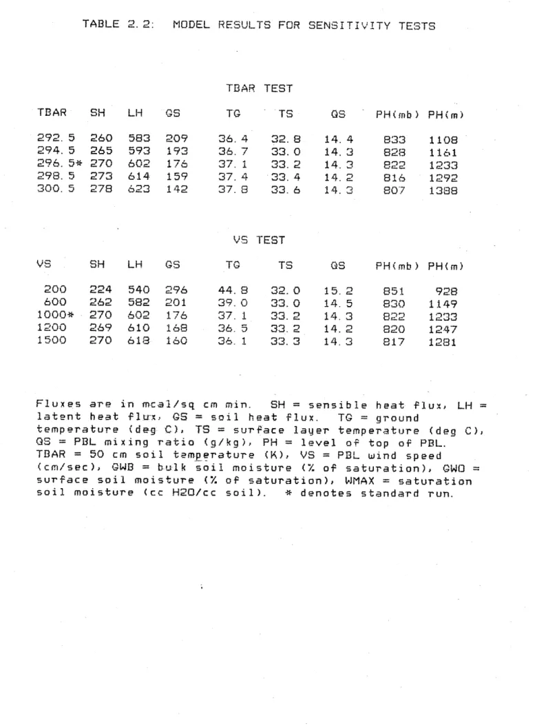
2.2 Model results for sensitivitu tests. 59

2.3 Model results for sensitivity tests (continued). 60

3. 1 Advection calculation for April case. 104

3.2 Model results at 21 GMT, 19 April. 105

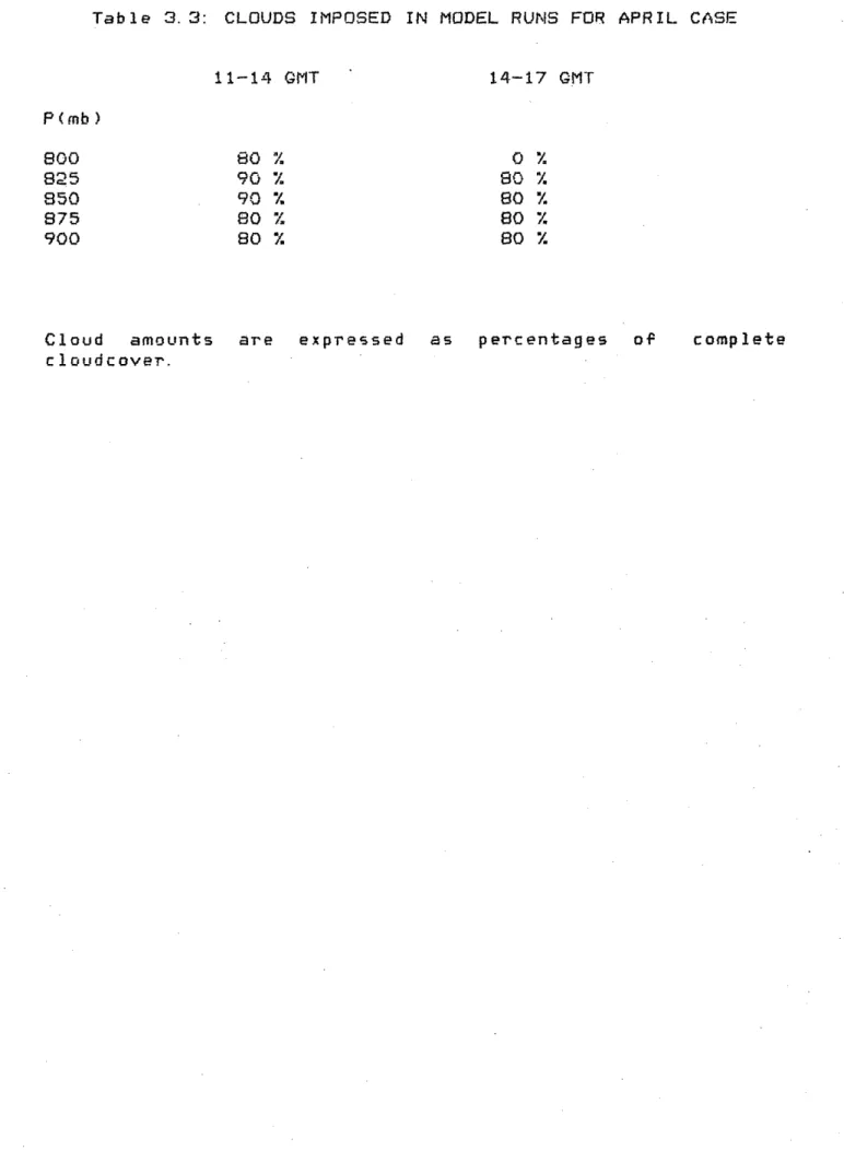
3.3 Clouds imposed in model runs for April case. 106 3.4 Imposed changes from Dodge City, Kansas including

inversion changes, for April 19. 107

3.5 Imposed changes from Goodland, Kansas including

inversion changes, for April 19. 108

3.6 Model results at 21 GMT, 19 April. 109

3.7 Sensitivity values for 21 GMT, 19 April model runs. 110

4. 1 Model results at 21 GMT, 9 May. 177

4.2 Clouds imp-os-ed in model runs for May case. 178 4.3 Imposed changes on model runs for May case. 178 4.4 Sensitiviztq values for 21 GMT, 9 May model runs. 179

4. 5 Model results at 23 GMT, 9 May. 180

4. 6 Model results at 23 GMT, 9 May, continued. 181 4.7 Sensitivity values for 23 GMT, 9 May model runs. 182 5. 1 Clouds imposed in model runs for June case. 247 5.2 Imposed changes on model runs for June case. 247

5. 3 Model results at 19 GMT, 6 June. 248

5. 4 Sensitivity values for 23 GMT, 6 June model runs. 249 5. 5 Negative area for 30-60 model run with imposed changes

INTRODUCTION

The term "convection" is used in meteorology to

•distinguish overturning motion in the atmosphere from laminar flows. As such, it includes a very broad class of atmospheric motion , which contains both buoyant and non-buoyant motion. For the purpose of this thesis, convection will be much more narrowly defined and will be used to denote only buoyant

overturning in the-atmosphere. The intent is to include only convection associated with severe weather in the central

section of the United.States. Although most severe weather is due to buoyant overturning, the association is not strict. Carbone (1982) reported on a case of nearly neutral

stratification which produced heavy rain and tornadoes.

Convecti-on in the- central U. S. in the spring is assumed to require the ...ol-lowing: un-stable thermal vertical

stra.tif-ication and an initiating (trigger) mechanism. The expected sequence is approximately as follows: Through large scale or mesoscale motion and/or heating and cooling

mechanisms, a section of the atmosphere becomes convectively unstable. This means that air parcels from the planetary boundary layer (PBL), if lifted sufficiently, would become positively buoyant, and would continue to rise in the

atmosphere. This requires abundant moisture, as the latent heat of condensation released in the parcel is needed to

maintain the parcel's buouancy. (The atmospheric lapse rate is almost always more stable than the dry adiabatic lapse rate over any appreciable layer.) There exists a stable layer above the PBL which separates the potentiallybuoyant air from the rest of the atmosphere. In the central U.S. this stable layer is very often characterized by a temperature inversion. Therefore, for convection to begin, a combination of heating and external dynamic forcing (trigger mechanisms) must act to

lift the potentially buoyant air through the stable layer where it will actually be buoyant. In a sense, this expected

sequence of events is incorrect. Actually, no parcels are lifted "through" the stable layer. What really happens is that a part o-f the PBL is destabilized by heating and/or adiabatic cooling of the inversion. This destabilization

occurs on a small spat-ial scale, much smaller than the scale of the observational -etwork. Hence, the appearance of the convection "breaking through" the stable layer is due to differences in s-cales.

Initiation of this type of convection has been studied for many years with varying emphases. Early work generally focussed on the problems of forecasting this type of weather. Convection is small scale in both space and time, which

presents very real forecasting and observational diffi-culties. Work by Fawbush et al. (195i) sought to characterize large

Their aids included vertical wind shear, low level temperature and moisture advection, and mid-level vorticity patterns.

Darkow et al.(1958) found a convincing statistical correlation between a. particular surface temperature pattern and the

occurrence of tornadoes. They showed that severe weather often occurred to the east and near the axis of a

tongue-shaped warm region. Other work sought to look at vertical stratification, with the development of various

indices to quantify instability or potential instability in the atmosphere. Thus, the Showalter Index (Showalter, 1953), the Lifted Index (Galway, 1956), and the Total Totals Index

(Miller, 1972) were spawned as forecast aides. This type of analysis continues to the present, with such work as Carlson

et al. (198) an-d- Moore (unpublished) in which new ways of quantifying vertical stratification have been developed which try to take into account more details in the structure. For instance, the-Shoimalter Index simply compares the temperature of air at 850 .rb when lifted adiabatically to 500 mb, with the ambient temperature at 500 mb. Carlson et al. (1980) developed an index called Lid Strength Index (LSI) which includes in addition to the Shawalter type of buoyancy, a measure of the

strength of the inversion which caps the PBL. This index would show a difference between places which have equal amounts of parcel b-uoyancy but have differing amounts of resistance to initiating the overturning motion.

Much work has focussed on determining what triggering mechanisms are operating i.n various situations. The result

has been the identification of several mechanisms, including ageostrophic frontogenetical convergence, gravity wave

triggering, sea breeze convergence, and outflow boundary convergence. As described by Koch and McCarthy (1982) the last of three groups of convection on 8 June 1974 seemed to be forced by frontogenetical motion along a cold front. In this instance the convergence and deformation along the

pre-existing front provided the vertical motion to set off the convection.

Work by Uccellini (1975) and later by Miller and Sanders (1930) implicated gravity wave forcing for severe

thunderstorms. Uccellini studied data from 18 May 1971 while Miller and Sander-s !o-k-ed at the so-called super-outbreak of tornadoes on 3 :April 1974. Both identified wave packets which

seemed to have coherent surface signatures through a large section of the east and central United States. They

correlated these packets with tornado occurrence and radar echo activity, and showed that the packets seemed to initiate or enhance convective activity as they moved across the

country. Koch and McCarthy (1982) also implicated gravity waves in the formation of the second convective outbreak in

their study of the 8 June 1974 case. In all of these examples the gravity wave packets triggered convergence in the PBL

which provided the lifting required to trigger the convection.

Sea breeze circulations have been shown to be important in triggering and organizing convection, particularly in-Florida. Cooper et al. (1932) showed clearlu that peninsula scale convergence due to the daily sea breeze triggered late morning convection. Coastlines are not the only places where sea breeze type circulations can be important. Sun and Ogura (1979) modelled a sea breeze type circulation using data from Oklahoma on 8 June 1966. A very strong temperature gradient formed in the vicinity of Norman, Oklahoma, and a convergence line emerged along this gradient in much the same way as a sea breeze. This "inland sea breeze" was a factor in the

triggering of the convection in this case.

Outflow- from other storms can act to trigger more

convection, through lifting in the manner of a density current bodily pushing the lighter air up. Maddox et al. (1980)

examined several cases in which tornadic thunderstorms intensified when they were in the vicinity of thermal boundaries. They theorized that convergence and cyclonic vorticity were enhanced along the boundaries, although they could not show this clearly. Matthews (1981) discussed a case where the outflow from a large convective storm triggered an arc cloud formation in which small convective cells were

Florida convection, showed that outflow contributed to convergence on a storm scale which was responsible for new cell growth. A particular case from 1973 in Florida was analyzed by Holle and Maier (1980). They showed that a tornado formed along an intersection of outflows from old cells, with convergence on the order of 10**-3 1/s.

In comparison to the work on dynamic forcing, the

creation of the convective instability has received much less attention in the published literature. The mechanisms

generally quoted or referred to are differential advection (warm low level, cold upper level) and boundary layer heating (BLH). Of the two,- more work on advection has been done. Modahl (1979) studied National Hail Research Experiment data from 1972 - 1974, for the occurrence of hail. He showed that two factors were most important: increased southerly winds to increase moist-u-re and heat in the PBL, and easterly winds to sustain the storms (and perhaps to give upslope triggering). Carlson e al. (1980) attempted to correlate convective

outbreaks with the strength of the capping inversion and the amount of potential instability (as discussed with the LSI above). For the case of 10 April 1979, they found good correlation between their fields of LSI and the convection. Davis and Scoggins (1981) used data from Atmospheric

Variability Experiment IV (AVE IV, 24-25 April 1975) to examine the creation of convective instability, wind shear,

and vertical motion. They considered all sources of convective instability except BLH. Interestingly, they discovered that all of the other sources (eg. large scale motions) contributed less than the residual, especially in the

surface - 850 mb layer. This implies that BLH, part of the residual, could have been the dominant term.

Some studies of convection in mountains suggested that low level advection of moisture was important (as above in Modahl, 1979), but some included BLH as a factor too.

Caracena et al. (1979) discussed the Big Thompson Storm in

which low level moisture was crucial to the storms sustenance, and upslope winds provided the lifting. Raymond and Wilkening (1980) examined dry convection over an isolated mountain, and found that the mountain was a large source of heat which

helped drive an upslope circulation. Although their case was dry, they speculated that an adequate moisture supply would certainly have led to thunderstorm formation over the

mountain. Cotton et al. (1982) studied a quasi-steady

thunderstorm which formed in the mountains in Colorado on 19 July 1977. They concluded that a combination of BLH, low

level moisture advection, and upslope winds initiated the convection.

These studies of convection in mountains have seemed to be more complete than those over the plains, although the BLH

contribution was still not clearly delineated. A study by Ogura et al.(1982) analyzed a convective system on 9-10 May 1.979 in the central United States. Their results suggested that BLH, inland sea breeze circulation and perhaps symmetric instability were responsible for the convection, a combination of thermodynamic and dynamic factors

The above discussion shows that initiation of convection by dynamic forcing occurs in many waus, sometimes many ways in the same place, within a few hours (Koch and McCarthy, 1982). It is apparent that the thermodynamic contribution to the convection se-quence has not been well quantified. One can speculate as to the reasons for the lack of work in this area: complex interactions between radiation, surface

characteristics, and boundary layer characteristics, plus large spatial variation in the physical constants (such as soil composition, albedo, vegetation, etc.). The problem is certainly difficult from the theoretical standpoint.

Additionally, some of the factors are not well observed, such as soil temperature and moisture.

The intent of this thesis is to quantify the relationship between BLH and the development of convective instability. The approach used is a combined observational and modelling

study of convective outbreaks occurring in three case studies

from

(SESAME). The cases of 19-20 April; 9-10 May, and 6 June 1979 are examined to determine the role of BLH in the creation of convective instability. For this purpose, convective

instability will be measured by the PBL lifted index (PLI). The PBL air is taken as a parcel with the mean potential

temperature and mixing ratio of the PBL.. The parcel is.lifted adiabatically to 500 mb, and its temperature is compared with the ambient 500 mb temperature. When lifted, unstable air will be warmer than the ambient atmosphere. The PLI is

positive for instability unlike the operational Lifted Index (Galway, -1956).

The PLI is- not the same thing as the surface lifted index (SLI, from Sanders, personal communication) in which parcels are defined by the surface observations. The PLI measures a mean PBL convective instability, above any superadiabatic

layers which may be present. For a clear, well-mixed PBL, the PLI can be as much as 4 degrees C lower than the SLI (Fort Sill, Oklahoma sounding at 1800 GMT, 6 June 1979, Fig.5.20), although generally the difference is closer to 2 degrees C. This difference raises an interesting question: which parcel really measures the cloud-scale convective instability which

is responsible for the initiation of convection? Cloud

modellers generally need very large perturbations to initiate convection, even with unstable soundings. On the other hand, it is difficult to envision that parcels can rise from the

surface layer through the entire turbulent PBL without dilution. Observations at the top of the clear PBL do not

show such large perturbations. I suspect that the answer is that parcels with characteristics in between the two extremes (mean PBL and surface layer), are more representative of the cloud-scale convective instability, being the result of

diluted surface layer parcels. Without attempting to settle this question, I shall use the mean PBL parcel definition to measure convective instability in this thesis.

The role of the stable layer is studied as well to

determine how much inhibition exists immediately prior to the convection. The inhibition is quantified by integrating the "negative area" on a pseudoadiabatic diagram.. This negative area is the region between the parcel's path on the chart, and the ambient sounding while the parcel is negatively buoyant. The energy equal to this area is found by calculating the work done by the negative buoyancy force per unit mass, =

S

well which must be surpassed for the parcel to realize its convective instability. If a PBL parcel were to rise through this negative area) it must have sufficient kinetic energy per unit mass, or an updraft velocity equal to (2*Negative

area)**1/2.

various physical paramenters have on the BLH. The model is one dimensional, and is designed to. model only effects of solar radiation on BLH. Incident radiation on the surface is divided into soil heat, sensible heat and latent heat fluxes. The effect of soil moisture plays a prominent, role in this part.- The. fluxes into the PBL drive turbulent entrainment at the top of the (assumed) well-mixed PBL , and the temperature height and moisture content of the PBL are computed. Above the PBL, atmospheric changes are inferred from observed sounding data and imposed on the model.

The term PBL will be used extensively throughout the rest of this thesis. It is not a well-defined term for the

atmosphere. As used in the following, it will refer to the part of the atmosp-hee which obtains most of its

characteristics. rom its proximity to the ground. Physically, this will meant-hat part of the atmosphere which is heated during the day by the fluxes from the ground surface. On an adiabatic chart,- the- well-mixed PBL will be identifiable by a dry adiabatic temperature lapse rate and a nearly constant mixing ratio (q) in the air nearest the ground.

In each of the three cases studied, the conditions prior to convection are analysed, and the location of the outbreak pinpointed. The model is then run using initial data from nearby soundings and varying the important parameters.

Various combinations of physical factors are applied and the effects on convective instability are determined. The

physical factors which are varied are ground wetness, presence of clouds, and changes in the atmosphere above te PBL. The factors are tried separately to determine individual

importance. Then combinations are tried, with the last runs including all of the relevant factors. If one of these last runs can reproduce the observed surface temperature and PBL moisture content, it will be regarded as a "correct" run in the sense that the included effects are modeled correctly. The model is described in detail in chapter 2. The three case studies follow in chapters 3,4,and 5. The last chapter,

THE MODEL

2.1: Introduction

One of the tools -used in this research is a

one-dimensional boundary layer model. The model is primarily used to determine and illustrate the role of -boundary layer heating (BLH) in the time evolution of soundings. It is run with and without various physical effects to quantify their importance in generating convective instability and/or

removing convective inhibition. The model is.also used to determine the vertical structure of the atmosphere at times and locations which did not have real sounding data (i.e. between stations and/or between sounding times). Although SESAME case stud-u days- were characterized by 3 hourly.

soundings on a rid spacing no larger than the normal synoptic grid and often sig.nificantly smaller, the convection often broke out "between" soundings in some way (time or space or both). Because of this, it was not possible to make

statements about the vertical structure of the atmosphere without some kind of supplementary information.

The convection primarily studied in this thesis occurred after much of the BLH took place. This means that the PBL

bottom of the PBL could be represented by known structure functions. Although strong horizontal thermal gradients were present by the outbreak time, the initial thermal gradients throughout most of the SESAME area, tended to be small, so that the initial conditions at any point could be specified with some certainty. The model then used these initial

conditions and predicted the thermal changes due to BLH for the rest of the model run.

2. 2: Atmospheric Structure

The PBL is assumed to be well-mixed in heat and moisture. A surface la-uer of five mb depth is assumed to exist. This is an ad hoc representation of the real structure, but the

surface layer is not of crucial importance in affecting the stability of the atmosphere. The PBL. above the surface layer is characterized by its potential temperature (well-mixed in heat = constant G ), its moisture (well-mixed in moisture = constant q) and its height in meters. The PBL is capped by an inversion which has a strength ( A& ) and a depth. The

initial inversion depth is taken from the input sounding. The top of the inversion is held constant until the PBL.grows

enough to absorb all of the inversion layer. The bottom of the inversion rises as the PBL grows by entraining air from the inversion layer into the PBL. The structure above the PBL is taken directly from the data in the original sounding. The

assumed structure is illustrated in Fig. 1.

2. 3: Conceptual Model Run

Detailed later are the various parameterizations used to effect changes in the initial atmospheric structure. They are

outlined here. Table 2.1 contains a schedule of the operations in the order actually used by the computer.

Radiative transfer is computed first. The incoming radiation at the top of the atmosphere is a function of time

of day and geographic location. Radiation is absorbed by water vapor, COV and liquid water (clouds). Some is

scattered, some is reflected. The atmosphere and the ground emit infrared radiation, and the net radiation is calculated for each laye-r in the atmosphere and the ground surface. .The net absorbed radiation in the ground is partitioned into.three parts: 1) soil heat flux, 2) sensible heat flux to the

atmosphere, and 3) Latent heat flux to the atmosphere. The soil temperature and moisture are changed to reflect the new surface energy balance. The PBL height and inversion strength change due to surface temperature changes and virtual sensible heat flux. The air temperature in the PBL is determined from the PBL characteristics, and the moisture (q) of the PBL is determined by a budget calculation for the PBL. The last changes made to the sounding are imposed changes above the

PBL. These can be derived trom known data (such as three hourly SESAME soundings) or predicted on the basis of current analysis. The model can be stopped and restarted to allow different imposed rates of change or changes in cloud cover. When a whole stable lay-er is absorbed by the PBL, a new stable layer is incorporated from the next higher level in the

sounding.

2.4: Radiation

The radiation parameterization is taken from Katayama (1972) and is a routine originally designed for use in the UCLA GCM. The model is described in brief here, and more

details are available in Appendix 7.1. The incident radiation and IR emission ar-e calculated separately. The net flux

divergence gives a mean temperature change for each model layer. The model incorporates an exponential fit to the data for specific humiditq to allow simple integration of water content. CO is included in a fixed form based on experimental data of Yamamoto (I952), and its contribution is then a

constant.

A. Incident Radiation

The influx of radiation is computed by starting with the solar constant and modifying it for albedo at the top of the

atmosphere. Scattered and absorbable radiation are computed separately, the fraction being assumed constant (35% available for absorption, 65% scattered to the ground). The scattered part of the incident radiation is corrected for multiple reflection between the atmosphere and the ground.

GL

.WDSt

SZT*

-

Z

where

So = solar constant = f(day of year) -- units of mcal/sqcm min

XT = zenith angle for time of day and location (radians)

cS = scattering albedo for atmosphere--if clouds are present they determine the scattering aledo

= albedo of ground surface = f(hour angle)

If a cloud layer is present, its presence is felt by both scattered and abs-orbable components. If the cloud is thick enough, and covers enough sky, incident radiation can be shut off. The model allows for variable amounts of cloud in each atmospheric layer expressed as a percentage. Only one layer of cloud is allowed, but it may be composed of one or several atmospheric layers of various percentage coverage. The model does not include any feedback mechanism to the cloud amounts,

hence these must be manipulated manually whenever the model run is stoppped and restarted. Atmospheric absorption by water vapor is calculated, using the sounding data for

specific humidity. Albedo at the surface is parameterized by a method from Wetzel (1978) w-hich allows for the change in

albedo depending on sun angle. The radiation which finally is absorbed in the soil becomes one component of the surface

energy balance. The absorbed part of the incident radiation at the ground is

GLW

.391 So., IT -

ABS

(.)

where ABS(i) = absorption in atmospheric layer i Total absorption at the ground is then

B. IR Emission

The equation of radiative transfer is solved subject to the boundary co-d4-itions .that downward infra-red (IR) flux at the top of the atmosphere is zero, and the upward IR flux at the earth's surface is t-he black body radiation at the surface temperature. We-ighted transmission functions are used,

corrected for the pressure dependence of absorption by defining an effective amount of an absorber. The total transmission function is assumed to be the product of the

individual ones for CO and H O. The following expressions for upward and downward fluxes at a particular height z are

* * * * IR = 7B - rB tn(u - u , T

)

" = mean total transmission function for effective absorber u# at temperature T

TC =-critical temperature which divides-the region of weak temperature dependence of T to that of strong

dependence of T

The weak region is 210 to 320 K for water vapor. So letting Tc = 220 K, the weak dependence region need only have a mean

temperature specified = T . Similarly, the upward flux is

7B

IR _u = irB _z + f g((u _{z- U, T) d('B)} T -- _(W'5) -B

z and the net upward flux

IR = IR - IRd *()

The only diff-iculty is determining the proper

transmission function near the particular level, where tau varies exponerrtially. The model uses an interpolation factor which is an empirical function of pressure, mixing ratio and

layer thickness. This allows proper calculation of tau

without a fine vertical mesh. The mean transmission functions are defined by empirical formulae at T,= 220 K and T = 260 K. Temperature dependence of tau for CO, is neglected, so a mean tau for CO is used based on pressure and amount of COi. The

distribution of CO,at each pressure level is a constant. The empirical functions for both absorbers were fit to data from Yamamoto (1952). For thick clouds, the top and bottom are assumed to radiate black body radiation at their respective temperatures, with no net flux inside.

2.5: Radiation Data Comparison

All of the expressions used for transmission coefficients and atmospheric absorption were derived from empirical data. After the model was assembled, it was run on sounding data to a) allow comparison with radiation measurements, b) allow

comparison with other more complex models, and c) allow variation of parameters such as aibedo and cloud amount to

ensure reasonable behavior.

Data for radiation measurements taken at O'Neill,

Nebraska in August and reported in Lettau and Davidson (1957), were available in Wetzel (1978). Fig.2.2 shows the

observations plotted over the radiation calculations from the model. The agreement is quite good, with a slight over

forecast near 1200 LST of about eight percent.

Three models were compared with the Katayama radiation routine. Rogers and Walshaw (1966) has been regarded as a classic parameterization for many years, so the IR

calculations were compared with it first. Fig. 2.3 shows the comparison for a sounding taken from Rogers and Walshaw. Notice that the agreement is very close. On Fig.2.4, three calculations are compared with the mod.el for an equatorial

sounding from London (1952). Although differences exist above 8 km, below that level, the present model is nearly in the middle of the scatter of the rest of the calculations. A

comparison is also made with a one-dimensional model.from Wetzel (1978). Wetzel's parameterization was run on the

O'Neill data, and the comparison is shown for net radiation on Fig.2.2. Again, the agreement is quite satisfactory.

The radiation model's cloud routine was tested for

qualitative behavior for thin and thick clouds. The results for the IR cooling- only appear on Fig.2. 5. For a very thick cloud, the top -f th-e cloud cools rapidly, while the bottom warms strongly. The cooling occurs because the flux for the top of the cloud only co-mes from relatively cool layers aloft, while no contribution comes through the thick clouds below. The cloud top radi-ates strongly to all layers above, so it has a net flux divergence. The opposite is true on the bottom of the cloud, which gives a net warming effect. The clear and partly cloudy cases deviate from the extreme in the expected way, with both the warming and cooling peaks losing intensity. Notice, however, that the sensitivity of the warming peak is much greater than that for the cooling peak. The partly cloud

condition still gives a strong cooling at cloud top, but very little warming below. Presumably, as the cloud barrier is removed, all of the cloud tends to radiate strongly to the lagers above. Not shown is the absorption of incident

radiation which greatly reduces the extreme values of cooling, giving net cooling at the cloud top of much lower magnitude.

2. 6: Surfa-ce Energy Balance

The surface energy balance at the surface- has the form

NR = SH + LH + GS (7)

where NR is the net radiation incident on the surface, SH is the sensible heat flux upward from the surface, LH is the latent heat flux upward from the surface and GS is the soil heat flux downward into the ground which heats the soil. Fig.2.1 illust-rates the various fluxes and their directions. NR is already known via the radiation routine. The rest are parameterized as follows.

A. Sensible and Latent Heat Fluxes

The sensible heat flux and latent heat flux (SH,LH) are parameterized using Monin-Obukhov similarity theory for the PBL. The fluxes depend upon the gradients in the surface layer, the depth of the boundary layer, and the incident

radiation . The theory assumes that the structure of

temperature and moisture .in the PBL have focrms which can be described by universal structurTe functions when scaled

equations are used. There are actually two structures

involved, since the PBL contains at least two distinct layers: the surface layer and the well-mixed layer. If the functions are required to be matched at their common boundary, the

following form results:

where

z = height above the ground zo = roughness length

h = t-he .d-pth of the boundary layer L = Monir/bukhov length

ft fl = uni-versa-! functions

The form of the temperature function is taken from Arya (1975). Details are in Appendix 7.2.

For stable boundarg layers, much scatter results when data are compared with theory . However, the present model is used only for unstable, well-mixed conditions. These

conditions give quite good agreement between theory and observations (Businger, et al., 1971). Furthermore, the

moisture function, f., is not well defined in the literature, and is usually assumed to be the same as the temperature

structure function. For-a well-mixed PBL this is likely a decent assumption, since both @ and q are nearly constant with height.

B. Soil Heat Flux

The soil heat flux (GS) is parameterized after Bhumralker (1975). Assuming vertical heat flux only, and that the

variation of surface soil temperature from an average

temperature is sinusoidal, one can solve the heat conduction equation to give eventually an expression for the soil heat

flux (see Appendix 7.2 for details). Evaluated at the surface,

LC

C V

I

_

T

T BA

)

where c = volumetric heat capacity of the soil TG = ground temperature

TBAR = some suitable average ground temperature

I1

S=-fre"uency of oscillation (= 2%/ 1 day)

2. 7: Ground Variables

Two parameters are crucial to the calculation of all of the components of radiation: TG and q(ground). These are parameterized by "force-restore": methods from Bhumralker

in Appendix 7.3. _{To find TO the heat conduction equation is} solved for a lager between 50 cm and 1 cm below ground

surface. This gives a prediction equation for TO

where

t 3

k

The soil moisture is found by assuming that surface soil moisture responds to three main processes: precipitation, evaporation, and flux from below. The bulk soil moisture

(GWB) is assumed to be constant over the period. According to DeardorffP (1977) the bulk soil moisture changes over a time scale of a few weeks, so GWB can certainly be assumed constant for a 12 hour period with little loss of accuracy. The

surface soil maisture is changed according to:

where

GWB = % bulk soil saturation (top 50 cm)

GW = " soil saturation

di = depth of diurnal cycle (=10 cm)

X = latent heat of evaporation 9s = density of H20 = 1 gm/cc WMAX = field capacity soil moisture

' = period of cycle

c Jc, are non dimensional constants

Deardorff's values for c and c 2were computed from data of Jackson (1973), measurements taken over bar-e soil near

Phoenix, Arizona in March.

.5 Cw t 7/o

Notice the middle value of c is a linear interpolation between the two extreme values.

2.8: Boundaru Laer Variables

The depth of the boundary layer (h) and strength of the inversion (A4) are predicted according to Zeman and Tennekes (1977). Their method assumes that the PBL depth changes due to turbulent entrainment of air above the inversion into the PBL. No allowance is made for the late afternoon collapse of the PBL, since the convective outbreaks occurred prior to this time. The energy comes from the virtual SH flux at the

surface, and the change of depth with time depends upon the strength of the inversion. They use the turbulent kinetic energy budget to develop a simple set of equations to describe this process. The equations which result are:

w = 9 h

*lr T

where

TS = surface temperature (top of surface layer) h = height of inversion

g = acceleration of gravity w. = convective velocity scale

VSH = virtual sensible heat flux at ground

and,

Wbv

S

where T = temperature gradient above the inversion W = Brunt-Vaisala frequency in the air above the

inversion \SH C - Cd bh c wZ T 5 t S 1+ gh AG

where VSHk = heat flux at the inversion (C 0 to give entrainment from above)

c&,cf ,c are dimenrsionless coefficients which are (from Zeman, 1975)

c. = O. 50 c& = O. 024 c = 3. 55 (1&)

In the case where 6 = O0 , no inversion exists and the

atmosphere presents no barrier to inversion rise. In this case, the model assumes a very small value fort8 A since the inversion must rise at a rapid but finite rate due to the turbulent entrainment. Finally,

These equations will allow the calculation of the necessary PBL characteristics. See Appendix 7.4 ?or a discussion of

their derivation.

2.9: PBL Temperature and Moisture

The final calculation to be performed is that for PBL values of T( i) and Q. These are found using the simple assumed structure in the PBL, and a budget for

0

calculated, so the amount of entrainment is known. This entrainment comes from the inversion layer, so the new depth of the inversion layer can be found. Using the new value for

Ae,

the lapse rate of potential temperature in the inversion, the potential temp-era-t-ure -of the PBL can be calculated. This then gives the new TS value, and the hydrostatic pressure level of the inversion hattom. Since the pressure depth of the surface layer is fixed,-- the height of the surface layer can be

computed hydrostatically. The process is illustrated schematically in Fig. 2.6.

2.10: Initialization Procedure

The model requires the initial sounding to have a specific form, to allow the model procedures to operate reasonably. In particular, a thin surface layer and a

well-mixed PBL above are both assumed. Realistically, the atmosphere is uniikely to possess either of these layers until later in the morning, especially in the presence of clouds. Nevertheless, the initial sounding must be forced to conform

immediately to the model requirements to prevent model collapse.

The initial sounding i down to near the surface. SESAME tapes at 25mb levels The first data point above-taken at a pr-essure level w mb (ie. 875mb or 950-Gb).

layers. So if this first d within 10 mb of the surface

s input as available from 400 mb. The data is available from the

! plus the surface-observation. the surface on the tapes is always hich is an integral multiple of 25 The model cannot handle very thin ata point above the ground is

pressure. it is rejected.

The surface observation is used to determine initial TS and GS in the model. These values are set at the top of the surface layer, 5mb above the ground. The ground temperature is initialized to be 0. 1 deg C higher than the surface

temperature to produce positive SH flux. The moisture for the PBL is set equal to the surface value. The PBL depth is

initialized at 90 m, measured from the ground. The atmosphere above 90 m, up to the first data point, is the first stable

layer. If this first stable layer is neutral, the stability is set to a minimal value to allow finite but fsst growth.

The delta theta for the first iteration is derived by

extending the first data point down to the 90 m level, and calculating its potential temperature. This process is shown on Fig. 2. 7. This operation creates an isothermal layer above the initial PBL, and the characteristics of this new layer are used to determine the value for T , the lapse rate in the stab.le air used in the model.

This initialization procedure seems like a major

modification to the sounding, but the actual changes are small enough to be barely detectable when plotted on a

pseudoadiabatic chart. These changes allow the mixed layer

model to work properyi. In addition: results from a study by Whiteman (1982) suggest that a small mixed layer appears

within 15 minutes of ground illumination, so the errors

associated with this initialization procedure should be small. For a typical sounding, the change in the dry static energy of

the adjusted portion of the sounding is less than 0. 1%.

2. 11: Sensitivity Tests

There are a number of constants used in this model, many of which are not easily evaluated. A number of sensitivity tests are performed to insure that these arbitrary constants are not controlling the results. The sounding used for this purpose is taken from a PBL Field project at O'Neill, Nebraska

on 13 August 1953. (This is the same sounding which has

already been mentioned in the radiation comparison discussion above. ) The sounding appears in Fig. 2.8. The standard run against which the others are compared uses the following values for the various constants: GWB = 90%, WMAX = 0.80 cc H20/cc soil, TBAR = 296.5 K, and VS = 1000 cm/s. In addition, initial GW (GWO) is varied, using 55% as the standard value. The results of the standard run appear in Figs.2.9 through 2.13. No clouds or other changes above the PBL are imposed in this or any of the other sensitivity runs.

The standard run is characterized by strong heating under moderately moist soil c.onditi6ns. The temperature of the

ground (Fig. 2. 13 rises rapidly during the day, peaking at 1400 local solar time (LST). The incident solar radiation (Fig. 2.10) is strongest at 1200 and begins to fall off

afterwards. The lag between the radiation peak and the ground temperature peak is due to the finite time required for the soil to heat. The soil is not in thermal equilibrium with the

incident radiation at noon, and so continues to heat under the decreasing but still strong radiation. The PBL moisture

(Fig. 2. 11) rises rapidly until near midday, in response to the latent heat flux (Fig. 2. 12). The LH flux in this run is

sufficient to strongly moisten the PBL. The air above the surface up to about 825 mb is very stable, and the PBL grows silowly, reaching 9325 mb very late in the run. The ground

temperature reaches 314 K, while the surface air temperature TS reaches 308 K shortly after. The moisture at this time is nearly 14 g/kg.

A. TBAR Test

TBAR is the diurnal average soil temperature, assumed constant with depth. At a depth equal to the L.imit of the diurnal variation (about 50 cm), TBAR = T(soil) independent of time. So TBAR can be regarded as a 50 cm soil temperature, assumed constant for the --iodel run. It is varied +/- 4 K from

the standard of 296.5 K. The results appear in Table 2.2. The timing of the peak values does not change over the range of TBARs, only the values themselves do. The fluxes show the greatest response, particularly the soil heat flux (almost +/-20%). Since -one of the two factors in the soil heat flux is the quantity TG-TBAR, the model's response to the change in TBAR is expected. Furthermore, the ground temperature

responds noticeably, showing a response of +/- 2 to 4%. The other parameters show little response, particularly the value for QS which hardly changes at all (+/- 0. 1 g/kg). TBAR does not have a great effect on the model output.

B. VS Test