FOR
IN-PIPE
WIRELESS
SENSOR
NETWORKS
George
Kokossalalus
S .M. Civil and Environmental Engineering Massachusetts Institute of Technology (2000)
Diploma of Civil Engineering
National Technical University of Athens (1998)
I
LIBRARIES
I
Submitted to the Department of Civil
and
Environmental Engineering
in partial fulfillment of the requirements
for the degree of
DOCTOR OF SCIENCE IN CIVIL
AND
ENVIRONMENTAL
ENGINEERING
//at
theebruary 2006
Institute of Technology.
Signature of Author.
.v..O......
t of Civil and Environmental Engineering January 15,2006
->
/
...
...
-
Certified by..
.,.
/ Eduardo KauselProfessor of ivil and Environmetal Engineering
4
Thesis SupervisorY - -
Accepted by..
...
.
,,
.-
...
Andrew J. Whittle Chairman, Departmental Committee for Graduate Students
ACOUSTIC
DATA COMMUNICATION
S Y S T E M
F O RIN-PIPE
George Kokossalakis
Submitted to the Department of Civil and Environmental Engineering on January 15, 2006 in partial fulfillment of the requirements for the degree of
Doctor of Science in Civil and Environmental Engineering.
ABSTRACT
Sustainability of ageing infrastructure is one of the greatest current civil engineering challenges, especially in the case of pipelines, where no direct access is available. Being simultaneously massive and distributed, their normal operation is critical for the health and prosperity of the community. In current practice, the condition of pipelines is assessed by non-destructive inspection techniques. Nonetheless, frequent pipeline failures warrant the continuous assessment of their condition, in order to schedule the maintenance activities accordingly, and assure their safe operation. Continuous monitoring necessitates the deployment of autonomous wireless sensor networks (WSN). This thesis proposes solutions for the communication and power units of a WSN for monitoring underground water pipelines.
Regarding the communication unit, it is proposed to use the pipeline as an acoustic waveguide for the transmission of appropriately modulated acoustic waves that encapsulate the digital data, since radio frequency transmission is not feasible underground. The confined acoustic channel imposes severe distortion on the propagating signal. In order to compensate for the dispersion and ambient noise, the proposed communication system employs an elaborate set of signal processing steps, such as Reed- Solomon Encoding, Barker Code Synchronization, Adaptive Equalization, Bandpass Filtering, Stacking and application of Inverse Transfer Function techniques. The robust performance of the proposed system is evaluated and verified by means of numerical simulations and scaled laboratory experiments. The bandwidth vs. power relationship is identified as the major trade-off for its design, since the in-pipe acoustic channel is bandwidth limited, while the WSN application is power limited. Excessive bandwidth use would impose severe distortion on the propagating signal, while power limitations restrict the use of bandwidth efficient digital communication techniques.
In order to address the power availability, a miniature power harvesting system, extracting energy from the flow of water inside the pipeline, is proposed, composed of a generator and a turbine combination. A hybrid design presenting the high efficiency of Gorlov's helical turbine and the high startup torque of Savonius turbine is provided. The resulting power harvesting system is capable of sustaining a continuous 1 watt of power under normal water pipeline operating conditions.
Thesis Supervisor: Eduardo Kausel
Acknowledgements
This work would not have been accomplished, without the collaboration of many individuals.
I am first indebted to my thesis supervisor, Prof. Eduardo Kausel, who supported my work and provided superior intellectual challenges. I have learned enormously from him and gained insight to numerous problems that I have encountered throughout this challenging experience. This work would not have been accomplished without his support, without the energy that he dedicated, both as a mentor and as a friend.
I would also like to thank Prof. Andrew J. Whittle for his constant encouragement and financial support. I am also thankful to Dr. Kevin S. Amaratunga, Prof. Jerome J. Connor, and Dr. John Germaine for their advice and willingness to assist in numerous tasks that arose throughout my doctoral the educational process. I am obliged to Dr. Ruaidhri M. O'Connor for his guidance and support in both my research and personal issues over the past 3 years.
I also feel that I owe a big thank you to the administrative staff of the Department, and especially to Cynthia Stewart, Pat Dixon, Anthee Travers, Joannie McCusker, Jeanette Marchoclu, Steven Rudolph, James Riefstahl and Alice Kalemluarian.
I am especially grateful to my close friends from Greece and MIT, who I will not name because I am afraid of not mentioning somebody important to me; however they are all written deeply in my heart. I would especially like to thank my friends in the US for the unforgettable experiences we have lived together, and for making my life at MIT enjoyable and my effort less tiring. I great thank you goes to my close friends in Greece for thinking of me and waiting patiently every holidays to welcome me back home. To my parents and sister I owe the most. This work would not have been possible without their continuous support and love. This thesis is dedicated to them, who have been the main source of my strength throughout this challenging period of my life.
Finally, I would like to thank my wife Dominic, who has been continuously there for me, supporting my efforts, and helping me overpass obstacles that I wouldn't have managed to, if I were on my own.
This work has been completed under the financial support of the Cambridge-MIT Initiative (CMI) under the grant 080P-IR FT, "New Technologies for Condition Assessment and Monitoring of Ageing Infrastructure". I am grateful for their support throughout my doctoral studies.
To my parents and sister who are always there for me.. .
Table of contents
...
CHAPTER 1
... ...
CHAPTER 2
...
.
.
.
...
STATE OF THE ART IN UNDERWATER ACOUSTIC COMMUNICATION
...
39...
2.1 INTRODUCTION 3 9
...
2.2 OPEN SEA ACOUSTIC COMMUNICATION 40
... 2.2.1 Signal Distortion 40 ... 2.2.2 Communication techniques 42 ... 2.2.3 Hardware 44 ... .
2.3 OPEN SEA
vs
IN-PIPE C O ~ I C A T I O N 48...
2.4 IN-PIPE ACOUSTIC APPLICATIONS 50
...
2.5 REFERENCES 5 2
CHAPTER 3
...
.
.
...
...
...
WAVE PROPAGATION IN PIPELINE WAVEGUIDES 57
...
3.1 INTRODUCTION 57
...
3.2 STATE OF THE ART FOR
w
PIPE WAVE PROPAGATION 58...
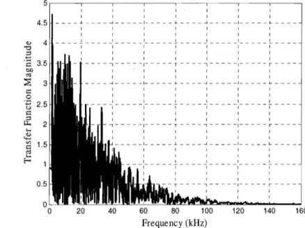
3 . 3 PIPELINE WAVEGUIDE SIMULATIONS 6 0
...
3.4 RIGID PIPE APPROXIMATION 62
...
3.4.1. Dynamic equations for a fluid 63
...
3.4.2. Hannonic point source in an unboundedfluid medium 65
... 3.4.3. Centered line source in a rigid cylindrical pipe: wave solution 67
...
3.4.4. Pipe with rigid walls: Source expansion into modes 70
...
3.4.5. Pipe with rigid walls: Off-center point source 73
...
3.4.6. Simulations 75
...
3.5 FLEXIBLE PPE EMBEDDED IN SOIL 9 3
...
3.5.1. Off-center source in a layered flexible pipe 94
3.5.2. Estimation of p* ... 95
...
3.5.3. Fluid cylinder subjected to external pressure 96
3.5.4. Fluid cylinder via stifiess matrix method ... 97
...
3.5.5. Graf addition theorem 102
... 3.5.6. Simulations 102 ... 3.6 CONCLUSIONS 112 ... 3.7 REFERENCES 114
CHAPTER 4
...
...
DIGITAL COMMUNICATIONS
....
...
..
...
...
117 ...4.1 INTRODUCTION 117
...
4.2 DIGITAL
vs
.
ANALOG COMMUNICATION 118...
4.3 DIGITAL COMMUNICATION SYSTEM COMPONENTS 121
...
4.4 MATHEMATICAL MODELS FOR COMMUNICATION CHANNELS 122
...
4.4.1. Additive White Gaussian Noise 123
...
4.4.2. Linear Time Invariant Filter 124
4.4.3. Linear Time Variant Filter ... 125 ...
4.5 DIGITAL COMMUNICATION TECHNIQUES 126
...
4.5.1. Formatting 126
...
4.5.2. Encoding 128
...
4.5.3. Mapping & Modulation 138
...
4.5.4. Equalization 148
...
4.5.5. Synchronization 155
...
4.6 TRADE-OFFS OF DIGITAL COMMUNICATION SYSTEMS 159
...
4.7 ADVANCED COMMUNICATION ISSUES 165
...
4.8 REFERENCES 167
CHAPTER 5
...
.
.
...
.
.
...
PROPOSED COMMUNICATION SYSTEM
... ...
169 ...5.1 INTRODUCTION 169
...
5.2 OPERATIONAL LAY OUT 170
... 5.3 SOFTWARE IMPLEMENTATION 172 ... 5.3.1 Message Formatting 172 ... 5.3.2 Encoding 174 ... 5.3.3 Modulation 175 ... 5.3.4 Synchronization 178 ...
5.3.5 Inverse Transfer Function 180
... 5.3.6 Stacking 183 ... 5.3.7 Bandpass Filtering 185 ... 5.3.8 Equalization 186 ...
5.4
HARD
WARE IMPLEMENTATION 187...
5.4.1 Microprocessor 188
...
5.4.2 Analog to Digital Converter 189
... 5.4.3 Signal Amplifier 190 ... 5.4.4 Transducers 190 ... 5.4.5 Power unit 193 ... 5.4.6 Installation 199 ... 5.5 REFERENCES 2 0 2 CHAPTER 6
... ...
SIMULATIONS... ...
2 0 56.2.1 Frequency Shifi Keying ... 207
6.2.2 Amplitude Ship Keying ... 211
6.2.3 Quadrature Amplitude Modulation ... 214
6.3 ENCODING ... 217
6.4 STACKING ... 221
6.5 ADAPTIVE EQUALIZER ... 2 2 8 6.5.1 Linear Equalizer ... 229
6.5.2 Decision Feedback Equalizer ... 234
... 6.5.3 Equalization of ASK and QAM signals 236 ... 6.5.4 Effect of pipeline waveguide on equalization process 240 ... 6.5.5 Equalization of higher data rate signals 244 ... 6.6 EFFECT OF AMBIENT NOISE 2 4 8 ... 6.7 CONCLUSIONS 2 5 1 ... 6.8 REFERENCES 255
...
CHAPTER 7 LABORATORY EXPERIMENTS...
.
.
...
2 5 7 ... 7.1 INTRODUCTION 2 5 7 ... 7.2 EXPERIMENTAL LAYOUT 2 5 8 7.3 HARDWARE ... 263 ... 7.4 RESULTS 2 6 9 ... 7.4.1 Straight Pipe 269 ... 7.4.2 Bent Pipe 277 ... 7.4.3 Branch Pipe 283 ... 7.5 REFERENCES 290 CHAPTER 8...
...
CONCLUSIONS 291List of Figures
Figure 1.1: In-pipe acoustic data communication
...
24Figure 1.2: Pipe bursts in Santa Monica and Boston [I], [2] . . .
.
. . ..
. . .. .
. . ..
. . 2 6 Figure 1.3: Examples of Pipeline Defects: root intrusion, and cross section blockage, [4].
... 2 9 Figure 1.4: Typical locations of fracture type of burst pipes, ([3] from Jones, 1983).
... .30Figure 1.5: Acoustic Emission ...
...
... ... ... 3 2 Figure 1.6: Components of an integrated wireless sensor node ... 33Figure 1.7: Typical Wireless Sensor Network Architecture . . .
. .
..
. ..
. . .. .
.. .
. . ..
. . ..
. . 3 5 Figure 2.1 : Volumetric absorption including all known relaxation processes, [4], [5] ..
.42Figure 2.2: Typical Transmitter - Receiver system.. .. . . ... . .. .. . .. . . .
..
. .. . . .. . . ..
. ..
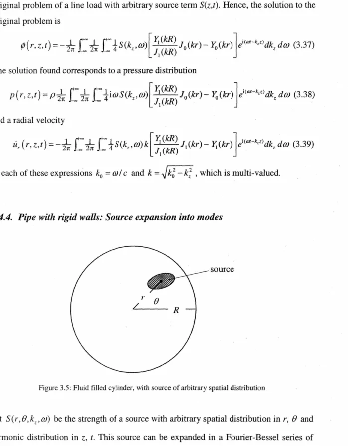
.. . . ... . .. .45Figure 2.3: Open - Sea acoustic modem (photo courtesy of Link Quest) ... 47
Figure 2.4: Published experimental performance of underwater acoustic telemetry systems. The channels vary from deep and vertical to shallow and horizontal. In general, the high rate or high range results are for deep channels while the cluster of low range, low rate results are for shallow channels. Modems developed by the research community are represented with diamonds while stars denote commercially available systems. The range x rate bound represents an estimate of the existing performance envelope. [2] ... 47
Figure 3.1 : Modes of Propagation inside hollow fluid filled elastic cylinders: Longitudinal waves ( L ) , Helical or Torsional waves (T), and Flexural waves (F).. 58
Figure 3 -2: Parametric Analyses to identify the effect of the transmission channel to the propagating signal . . .
. .
..
. . ..
..
. . .. . .
. . .. . .
..
,. .
. . ..
. ..
. . ..
. .. . .
. ..
. . , . . . ..
. .. .
. . . . 6 1 Figure 3.3: Azimuthally distributed modes of propagation Regions of uniform phase: (a) along the cross section, [31], (b) along the pipe length ... 63Figure 3.4: Bessel Functions of the (a) first Jn and (b) second Yn lund, [32] ... 68
Figure 3.5: Fluid filled cylinder, with source of arbitrary spatial distribution ... 70
Figure 3.6: Off-center source in pipe with rigid walls ... 73
Figure 3.7: Excitation Waveforms . . .
.
. . .. .
. . ..
. . .. . . .
..
. . ..
. ..
. ..
..
. . . 7 7 Figure 3.8: Frequency Spectrum (a) Single squared sinusoidal pulse, (b) Tapered group of sinusoidal waves...
....
... 77Figure 3.9: Attenuation vs. Distance; Pressure Time Bstory and Frequency Response Spectrum for R = 0.5m, a = r = Om,
f,
= 5kHz, and (a)z
= lOm, (b)z
= loom, and (c)z
= 500m ... 78Figure 3.10: Attenuation vs. Frequency; Pressure Time mstory and Frequency Response Spectrum for R = 0.5m, a = r = Om,
z
= 10m, and (a) f, = IkHz, (b)f, = 5kHz, and (c) fo = 20kHz ... 79Figure 3.11: Transfer Function for a pipeline with R = 0.5m, at a distance
z
= lorn, for the n = 0 solution containing the first 50 modes ... 80Figure 3.12: Transfer Function for a pipeline with R = lm, at a distance
z
= lorn, for the n = 0 solution containing the first 50 modes ... ....
81Figure 3.13: Dispersion Curves for n = 0 and (a) R = 0.15m, (b) R = 0.5m and (c) R = l m ... 83
Figure 3.15: Effect of pipeline radus; Pressure Time Histories for
z
= 10m, a = r = R, fo...
= 5kHz and (a) R = 0.15m7 (b) R = 0.5m and (c) R = l m 85 Figure 3.16: Effect of pipeline radius; Pressure Time Histories for
z
= 10m, a = r = R, fo= 5kHz and (a) R = 0.15m, (b) R = 0.5m and (c) R = l m [Close up of Figure 3.151
...
85 Figure 3.17: Pipe Radius vs. modes of propagation; Pressure Time Histories forz =
10m, a = r = R, f o = 1.5lcHz and(a) R=0.15m7 (b) R=0.5m and (c) R = l m...
86 Figure 3.18: Effect of damping; Pressure Time Histories forz
= 10m, R = 0.5m, a = r =R, fo = 5kHz, and (a) < = 0.5%, (b) < = 1% and (c)
r=
5% ... 88 Figure 3.19: Pressure Time History of the direct and scattered signals arriving at thereceiver for fo = 1.5kHz, and R = 0.5m,
z
= lorn, a = r = R, (a)z, =
5m, and (b)zs
= l m or 9m...
90 Figure 3.20: Pressure Time History of the direct and scattered signals arriving at thereceiver for fo = 5kHz, and R = 0.5m,
z
= IOm, a = r = R, (a)z, =
5m, and (b)zS
= l m or 9m...
91 Figure 3.21: Pressure Time =story of the direct and scattered signals arriving at thereceiver for fo = 20kHz, and R = 0.5m, z = 10m, a = r = R, (a) zs = 5m, and (b) t = l m or 9m
...
92...
Figure 3.22: Flexural modes, [34] 9 4
Figure 3.23: Two stage solution for flexible pipe embedded in soil (a) Source and
...
inward pressure p* , (b) Outward traction p* 9 5
...
Figure 3.24: Graf addition theorem.. 102
Figure 3.25: Attenuation vs. Distance; Pressure Time History and Frequency Response Spectrum for R = 0.5m, a = r = R, fo = IkHz, Cs = 0.2 kmlsec, t = 2cm, and (a)
z
=...
lOm, (b)
z
= 100m 104Figure 3.26: Pressure Time History and Frequency Response Spectrum for the tapered sinusoidal waveform excitation and R = 0.5m, a = r = R,
z
= 10m,fo = 1.5kHz,
C, =...
0.2 km/sec, and t = 2cm 105
Figure 3.27: Attenuation vs. Frequency; Pressure Time History and Frequency Response Spectrum for R = 0.5m7 a = r = R,
z
= 10m, Cs = 0.2 W s e c , t = 2cm, and (a)fo =...
2kHz, (b) fo = 5kHz and (c) fo = 20kHz 106
Figure 3.28: Pressure Time History and Frequency Response Spectrum for z = 10m, fo =
...
1 kHz, a = r = R, C S = 0 . 2 W s e c , and(a) R =0.15m, and (b) R = l m 107 Figure 3.29: Effect of soil stiffness; Pressure Time History and Frequency Response
Spectrum for
z
= 10m,fo = 1 kHz, R = 0.5m, a = r = R, t = 2cm, and soil acoustic...
wave velocity (a) C, = 0 (No soil), and (b) Cs = 2 km/sec 109 Figure 3.30: Radiation Damping (Pressure Time History for n = 0, z = 10m, fo = 1 kHz,
...
R = a = r = 0.5m, and C, = 0, 0.2, and 2 km/sec) 110
Figure 3.31: Effect of pipeline thickness; Pressure Time Kstory for
z
= 10m, fo = 1 kHz, R = 0.5m, a = r = R, Cs = 0.2 km/sec and pipe wall thickness (a) t = 5mm, and (b) t-
- 1Ocm ... 11 1 Figure 3.32: Effect of pipeline material; Pressure Time History and Frequency Response
Spectrum for PVC pipe with
z
= 10m, fo = 1 kHz, R = 0.5m, a = r = R, Cs = 0.2 ...kmlsec 1 12
...
Figure 4.1 : Morse code, [I]. 1 18
...
Figure 4.3. Traditional components of a digital communication system. [2]
...
122Figure 4.4. Additive Noise Model ... 123
Figure 4.5. Linear time invariant filter model ... 125
Figure 4.6. Linear time variant filter model ... 125
Figure 4.7. Common Signal Processing Steps of a Digital Communication System .... 126
Figure 4.8. 5-Bit Baudot Code, [I] ... 127
Figure 4.9: 7-Bit American Standard Code for Information Interchange (ASCII). [4] . 127 Figure 4.10. Linear Block Codes ... 134
Figure 4.11. Pulse coded modulation waveforms. [4] ... 141
Figure 4.12. ASK signal constellation
...
143Figure 4.13. ASK waveform
...
144... Figure 4.14. PSK Signal Constellations 145 ... Figure 4.15. PSK waveform 145 Figure 4.16. QAM signal constellations ... 146
Figure 4.17. QAM waveforms ... 146
... Figure 4.18. FSK representation in the frequency plane 147 ... Figure 4.19. FSK waveform 147 ... Figure 4.20. Linear Adaptive Equalizer 150 ... Figure 4.2 1 : Transversal filter detail 150
...
Figure 4.22. Decision Feedback Equalizer 151...
Figure 4.23. Phase Locked Loop 156 Figure 4.24: Bit error probability PB versus Signal to noise ratio per bit E O o for coherently detected M-ary signaling: (a) orthogonal signaling, (b) Multiple phase...
signaling. [4] 161 Figure 4.25: Bandwidth efficiency q, in bit/s/Hz as a function of SNR per bit, for -5 ... constant symbol error probability of 10 , [3] 163 Figure 4.26: Bandwidth of digital data, [4]. (a) Half Power, (b) Noise equivalent, (c)
Null to Null, (d) 99% of Power, (e) Bounded Power Spectral Density at 35 and 50 dB...
164... Figure 5.1 : Operational diagram of proposed digital communication system 170 ... Figure 5.2. Transmitter and receiver hardware diagram 171 Figure 5.3: 7-Bit American Standard Code for Information Interchange (ASCII), [I]
.
173 Figure 5.4: Bandwidth efficiency q, in bit/s/Hz as a function of SNR per bit. for constant 5.
... symbol error probability of 10- [2] 177 Figure 5.5. Example of signal with Barker Code illustrating silent time t ... 179Figure 5.6: Azimuthally distributed modes of propagation Regions of uniform phase along the cross section for the first mode of each of the first 4 orders ... 184
Figure 5.7: Beam Patterns (a) Omnidirectional. (b) Hemispherical. (c) Toroidal. and (d) Conical. [9] ... 192
Figure 5.8. Volumetric absorption including all known relaxation processes. [12] ... 195
Figure 5.9. Power harvesting system from the flow of water inside the pipeline ... 197
Figure 5.10: (a) Gorlov's Helical Turbine. (b) Savonius Turbine. [17]. (c) Hybrid Design ... 198
...
Figure 5.1 1: Examples of Pipeline Robot Configurations. [18] 200
Figure 6.1 : Amplitude and Frequency Response of Transmitted Signal for FSK
...
Figure 6.2: Pressure Time History and Frequency Response of Received Signal from a pipeline waveguide with R = a = r = 0.5m7
z =
10m for FSK modulation at data rates (a) lkbps, (b) 4kbps and (c) 7kbps ... 209 Figure 6.3: Synchronization with Barker Code, Matched Filter Response (a) Theoretical,...
and (b) Actual.. 2 10
Figure 6.4: Amplitude and Frequency Response of Transmitted Signal for ASK
modulation at data rates (a) lkbps, (b) 4kbps and (c) 7kbps ... .212 Figure 6.5: Pressure Time History and Frequency Response of Received Signal from a
pipeline waveguide with R = a = r = OSm, = 1Om for ASK modulation at data
...
rates (a) lkbps, (b) 4kbps and (c) 7kbps 2 1 3
Figure 6.6: Signal Constellations for ASK modulated signals (a) lkbps, (b) 4kbps, and (c) 7kbps
...
214 Figure 6.7: Amplitude and Phase of Transmitted Signal for QAM at data rates (a) lkbps, (b) 4kbps, and (c) 7kbps ... 215 Figure 6.8: Pressure Time fistory and Signal Constellation of Received Signal from apipeline waveguide with R = a = r = 0.5m,
z =
1Om for QAM at data rates (a)...
1 kbps, (b) 4kbps, and (c) 7kbps 2 1 6
Figure 6.9: Amplitude and Frequency Spectrum of Transmitted signals for FSK
modulation of encoded messages at data rates (a) lkbps, (b) 4kbps, and (c) 7kbps.
...
219 Figure 6.10: Pressure Time History and Frequency Response of Received Signal from apipeline waveguide with R = a = r = 0.5m,
z
= 10m for FSK modulation of encoded ... messages at data rates (a) 1 kbps, (b) 4kbps, and (c) 7kbps 220 Figure 6.11: Pressure Time &story and Frequency Response of Received Signal at thebottom of a pipeline waveguide with R = a = r = 0.5m,
z
= lorn for FSK modulation...
of encoded messages at data rates (a) lkbps, (b) 4kbps and (c) 7kbps 222 Figure 6.12: Stacked Signal by addition of received signals at crown and bottom of pipe.
Pressure Time fistory and Frequency Response for FSK modulation at data rates (a) lkbps, (b) 4kbps and (c) 7kbps
...
223 Figure 6.13: Stacked Signal by subtraction of received signals at crown and bottom ofpipe. Pressure Time fistory and Frequency Response for FSK modulation at data
...
rates (a) lkbps, (b) 4kbps and (c) 7kbps 2 2 3
Figure 6.14: Transfer Functions of the first four orders of modes for a pipeline
waveguide with R = 0.5m and
z
= 10m...
226 Figure 6.15: Pressure Time &stories and Frequency Response of FSK modulated signalat 0.4kbps data rate for a pipeline waveguide with R = a = r = 0.5m,
z
= 10m (a) Transmitted signal, (b) Received signal at the crown, and (c) Stacked signal...
generated by addition of top and bottom recorded signals 228
Figure 6.16: Example Pressure time history and Frequency response of (a) inadequate length and (b) poorly trained Linear Adaptive Equalizer using the LMS filter tap
...
weight adaptation algorithm for FSK modulated signals at lkbps data rate .23 1 Figure 6.17: Pressure time history and Frequency response of Linear Equalizer using the
LMS filter tap weight adaptation algorithm for FSK modulated at data rates (a)
...
Figure 6.18: Pressure time history and Frequency response of Linear Equalizer using the RLS filter tap weight adaptation algorithm for FSK modulated signals at data rates (a) 1 kbps, (b) 4kbps and (c) 7kbps ... 2 3 3 Figure 6.19: Pressure time history and Frequency response of DFE using the LMS filter
tap weight adaptation algorithm for FSK modulated signals at data rates (a) lkbps,
...
(b) 4kbps and (c) 7kbps 235
Figure 6.20: Pressure time history and Frequency response of DFE using the RLS filter tap weight adaptation algorithm for FSK modulated signals at data rates (a) lkbps,
...
(b) 4kbps and (c) 7kbps 235
Figure 6.21: Pressure time history, Frequency Response, and Signal Constellation of DFE using the LMS filter tap weight adaptation algorithm for ASK modulated
... signals at data rates (a) 1 kbps, (b) 4kbps, and (c) 7kbps ,237 Figure 6.22: Pressure Time History and Signal Constellation of received and equalized
signals with DFE using the LMS filter tap weight adaptation algorithm for QAM
...
modulated signals at data rates (a) lkbps, (b) 4kbps, and (c) 7kbps 239 Figure 6.23: Pressure Time History and Frequency Response of Received Signal for
FSK modulation at 4kbps data rate for propagation distance
z
= 10m and pipeline ...radius (a) R = 0.15m, and (b) R = l m 241
Figure 6.24: Pressure time history and Frequency response of DFE using the LMS filter tap weight adaptation algorithm for FSK modulated signals at 4kbps data rate, for a propagation distance of
z
= 10m in a pipe with radius (a) R = 0.15m and (b) R = l m... 242 Figure 6.25: Pressure Time a s t o r y and Frequency Response of Received Signal for
FSK modulation at 4kbps data rate for pipeline radius R = 0.5m and propagation ...
distance (a) = loom, and (b)
z
= 500m 243Figure 6.26: Pressure time history and Frequency response of DFE using the LMS filter tap weight adaptation algorithm for FSK modulated signals at 4kbps data rate inside a R = 0.5m pipeline for a propagation distance of (a) t = loom, and (b)
z =
500m2 4 4 ...
...
Figure 6.27: Formatting and encoding of textual message 245
Figure 6.28: Amplitude and Phase of Transmitted Signal for QAM at data rates (a) 12kbps, and (b) 2 1 kbps ... 2 4 6 Figure 6.29: Pressure Time &story and Signal Constellation of Received Signal and
equalized signals with DFE using the RLS adaptation algorithm for QAM at data rates (a) 12kbps, and (b) 2lkbps inside a pipeline waveguide with R = a = r = 0.5m,
z
= lorn.. ... .247 Figure 6.30: Effect of Ambient noise on transmitted signal; Pressure Time History andFrequency response for FSK modulated signal at 4kbps data rate for SNR equal to ...
(a) lOdB, (b) 2dB, and (c) OdB 249
Figure 6.31: Effect of Ambient noise on transmitted signal; Pressure Time History and Frequency response for FSK modulated signal at 4kbps data rate for SNR equal to
...
(a) IOdB, (b) 2dB, and (c) OdB 250
Figure 7.1: Laboratory Experiment Pipeline layout (a) Straight, (b) Bend, (c) Branch 259 Figure 7.2: Simulated Pressure Time Histories single pulse transmitted inside a (a) 4"
.. diameter, 10m long PVC pipe, and (b) l m diameter, lOOm long cast iron pipe. 262 Figure 7.3 : Schematic Diagram of Laboratory Experiment Hardware Configuration . .263
Figure 7.4: (a) Speaker and (b) Microphone used as transmitter and receiver and
...
corresponding frequency response, [I] 2 6 5
...
Figure 7.5: Speaker Amplifier 2 6 6
...
Figure 7.6: Microphone supporting circuit and preamplifier 2 6 7
Figure 7.7: Pressure Time History and Frequency Response of Laboratory Experiment for 30 ft propagation distance in straight pipe of FSK modulated signals at data
...
rates (a) lkbps, (b) 4kbps, and (c) 7kbps 2 7 0
Figure 7.8: Transfer Functions of the 30 feet straight pipe laboratory experiment for the first 9 orders of modes
...
271 Figure 7.9: Pressure Time &story and Frequency Response of Stacked signal generatedby subtraction of the crown and bottom recordings for the 7kbps FSK modulated signal in a 30ft straight pipe
...
272 Figure 7.10: Pressure Time History and Frequency Response of equalized signal with aDFE utilizing the RLS adaptation algorithm for FSK modulated signals at data rates (a) lkbps, (b) 4kbps, and (c) 7kbps
...
273 Figure 7.11 : Pressure Time History and Frequency Response of 7kbps FSK transmittedsignal for simulated laboratory experiment of air filled 30 feet long and 0.05m in radius PVC pipe
...
274 Figure 7.12: Pressure Time mstory and Frequency Response of received and DFE...
equalized FSK 7kbps signal for propagation distance 10 feet 275
Figure 7.13: Pressure Time History and Frequency Response of (a) received, (b) stacked by subtraction, and (c) DFE equalized, 7kbps ASK modulated signal for 30 ft propagation distance in straight pipe
...
276 Figure 7.14: Pressure Time mstory and Signal Constellation of (a) received, (b) stackedby subtraction, and (c) DFE equalized, 7kbps QAM modulated signal for 30 ft propagation distance in straight pipe ... 277 Figure 7.15: Pressure Time fistory and Frequency Response of a 30ft bent pipe
Laboratory Experiment for FSK modulated signals at data rates (a) lkbps, (b) ...
4kbps, and (c) 7kbps 2 7 8
Figure 7.16: Qualitative explanation of transmission loss near to the frequency at which
...
the wavelength equals twice the pipe diameter, [2] 279
Figure 7.17: Pressure Time History and Frequency Response of Stacked signal generated by subtraction of the crown and bottom recordings for the 7kbps FSK modulated signal propagating inside a 30ft bend pipe
...
280 Figure 7.18: Pressure Time &story and Frequency Response of equalized signal with aDFE utilizing the RLS adaptation algorithm for FSK modulated signals at data rates
...
(a) 1 kbps, (b) 4kbps, and (c) 7kbps. 2 8 1
Figure 7.19: Pressure Time &story and Frequency Response of (a) received, and (b) DFE equalized, 7kbps ASK modulated signal for 30 ft propagation distance in a bent pipe
...
282 Figure 7.20: Pressure Time libstory and Signal Constellation of (a) received, and (b)DFE equalized, 7kbps QAM modulated signal for 30 ft propagation distance in a ...
bent pipe.. .282
...
Figure 7.22: Pressure Time History and Frequency Response of Laboratory Experiment for 30 ft propagation distance in branched pipe of FSK modulated signals at data rates (a) lkbps, (b) 4kbps, and (c) 7kbps
...
284 Figure 7.23: Pressure Time &story and Frequency Response of branch pipe receivedsignal from 30ft branched pipe Laboratory Experiment for FSK modulated signals
...
at data rates (a) lkbps, (b) 4kbps, and (c) 7kbps 285
Figure 7.24: Pressure Time History and Frequency Response of Stacked signal generated by subtraction of the crown and bottom recordings for the 7kbps FSK modulated signal in a 30ft branched pipe
...
287 Figure 7.25: Pressure Time History and Frequency Response of equalized signal with aDFE utilizing the RLS adaptation algorithm for FSK modulated signals at data rates (a) lkbps, (b) 4kbps, and (c) 7kbps. ... 2 8 8 Figure 7.26: Pressure Time History and Frequency Response of (a) received, (b) stacked
by subtraction, and (c) DFE equalized, 7kbps ASK modulated signal for 30 ft propagation distance in a branched pipe ... .288 Figure 7.27: Pressure Time =story and Signal Constellation of (a) received, (b) stacked
by subtraction, and (c) DFE equalized, 7kbps QAM modulated signal for 30 ft propagation distance in a branched pipe ... 289
List of Tables
Table 4.1 : Barker Codes ... 159 Table 5.1 : Barker Codes ... 180 Table 6.1 : Error Performance before and after decoding of Crown, Bottom and Stacked
signals for FSK modulation ... 2 2 4 Table 6.2. Bit error rates following the signal processing blocks of the receiver ... 253 Table 7.1 : Acoustic wave velocity and density of Water, Cast Iron, Air, and PVC
...
261Chapter 1
Introduction
1.1
Thesis Objectives
Digital communication systems are nowadays used in every aspect of human life and operations. Cell phones, television broadcasts, global positioning systems, internet, to name a few, are examples of applications employing digital communication techniques. In essence, any operation requiring data exchange of some sort utilizes digital systems, due to their inherent reliability and effectiveness. Digital data can be reproduced accurately very easily even after severe distortion while there exist an abundance of error correction algorithms that preserve the robustness of the communication system even under extreme events. In parallel with the emergence of digital communication systems, monitoring is currently a very active area with an enormous number of potential applications, ranging from wildlife to instrumentation and operation to infrastructure monitoring. Especially the latter one has become the center of attention in many due to sustainability and homeland security concerns.
Within the context of monitoring infrastructure, the scope of this thesis is to implement and evaluate an acoustic digital data communication system for use with in- pipe wireless sensor networks. The term wireless at this point it is used to express a tetherless connection rather than the commonly used radio frequency communication. The proposed communication system uses appropriately modulated acoustic waves, in the place of electromagnetic waves, since pipelines are typically laid underground and radio frequency transmission is not feasible.
More explicitly, the objective of this research work is to prototype the communication unit of a monitoring sensor system, as shown in Figure 1.6. The proposed communication system is based on the exchange of acoustic signals between stationary nodes in a sensor network, through the water flowing in the pipeline. The pipe will be used as an acoustic wave guide, while underwater acoustic transducers will both generate
and record appropriately formed and modulated acoustic signals to carry data, see Figure 1.1. Once generated, these waves will propagate through the water inside the pipe and can be detected by a receiver at the remote location. The target distance of this data communication system is in the order of 300 to 500 m, while the bit rate is on the order of
lkbps.
Source
/-
Receiver Figure 1.1 : In-pipe acoustic data communicationDuring propagation the acoustic wave undergoes several distorting phenomena, which alter its shape, amplitude, frequency or phase characteristics. Two are the major signal distortion mechanisms of the in-pipe waveguide, namely ambient noise and dispersion. Ambient noise refers to the addition of a random signal of specific mean value and variance. Dispersion corresponds to a number of phenomena, such as multipath propagation, that cause signal reverberation and time spreading, as well as phase and frequency shift. The delayed arrivals of the propagating signal may overlap destructively causing severe signal attenuation, or signal fading. Channels presenting such behavior are referred to as fading channels.
In such a confined environment, as the inside of a pipeline, high dispersion and attenuation of the signal is anticipated, mainly because high frequency signals will excite many modes of vibration, which successively propagate at different speeds. Furthermore, there is loss of signal into the surrounding medium as well as reverberation of waves at points of discontinuity, such as pipe joints and bends. Thus, in order to achieve reliable transmission, the data communication system should employ dispersion compensation and error correction algorithms. Ideally, such a system should operate under the additional restriction of limited power supply.
Under the aforementioned considerations along with any additional environmental limitations and digital communication technique restrictions the current thesis constitutes
essentially a feasibility analysis on the idea of acoustic communication using a water pipeline as the transmission channel. The conclusion of the research is expected to propose and evaluate the performance of a communication system that addresses all the issues mentioned above and discussed in detail in the Chapters to follow. It will be seen that the successful completion of this research work involves resolution of several c:onflicting issues.
1.2
Motivation
The basic concepts related to the motivation supporting the objectives of this thesis can be expressed in four basic steps; (a) the primal problem that needs to be addressed is pipeline monitoring, (b) the proposed solution is to deploy wireless sensors in a network arrangement inside the pipelines, (c) the problem in deploying wireless sensor networks is that wireless communication in terms of radio frequency is not feasible underground, while the availability and long term sustainability of power is scarce, (d) this thesis addresses these two problems with emphasis on the former one. Four major questions directly arise; why study pipeline problems, why use monitoring; why install sensors inside the pipeline, and why do we need wireless communication. Justification to these questions is provided in the following paragraphs.
Why pipelines?
One of the greatest challenges that the science of civil engineering is facing nowadays is to preserve the safe operation of ageing infrastructure. This challenge is further aggravated for underground networks such as pipelines, where no direct access is feasible. Being simultaneously massive and distributed, their normal operation is critical for the health and prosperity of the community, while providing water, oil, gas, and steam supply, as well as sewage removal, they affect the functioning of whole cities.
The vast majority of this infrastructure was constructed more that 50 years ago, when both the long-term performance of the materials used was hardly known, and the methods applied were not technologically advanced enough, to ensure material production and on site construction uniformity. As a result, not only nowadays is there
clear evidence that this infrastructure is highly deteriorated - since pIpe bursts are frequent - but also the fragility of old pipelines constitutes a major problem in congested urban environments. This is supported by the recent pipeline bursts in Santa Monica and Boston presented in Figure 1.2.
Figure 1.2: Pipe bursts in Santa Monica and Boston [1], [2]
Due to the nature of this infrastructure, it is practically impossible to monitor its
current. state in detail. Nonetheless, the financial and the societal cost of associated
failures is usually enormous: floods, large surface settlements, waste water leakage, cease of clean water supply, even loss of human life are only some of their catastrophic
consequences. Even further, the recent terrorist attacks indicate the potential of using
these facilities as means for mass destruction.
The proposed wireless sensor monitoring system will be deployed to fresh water pipelines; despite their critical importance for the public health and quality of life, fresh water networks are among the oldest infrastructures currently in use, with very frequent
failures and enormous associated replacement and maintenance cost. Based on this
reasoning water pipelines were selected among other infrastructure for the deployment of
the proposed wireless sensor network. However, the outcome of this thesis can be
projected and extended to applications related to other pipeline networks.
Why monitoring?
The quick answer to this question is that continuous monitoring of water pipeline networks is necessary because inspection is not enough. All of the aforementioned issues suggest that it is critical for these networks to be continuously assessed, to predict their long term behavior, to extend their remaining life, to schedule the maintenance activities accordingly, and assure their safe operation. In current practice, the condition of pipelines is assessed by inspection techniques, as discussed in a subsequent paragraph. Nonetheless, the processes, events or conditions that lead to catastrophic failures of pipelines frequently occur in between two scheduled inspections, rendering the constant monitoring of critical pipelines necessary. This monitoring capability can be provided through careful selection of the system installation combined with the recent advances in wireless sensing, which leads to the two final questions.
Why inside?
The installation of monitoring system inside the pipeline provides a number of advantages. First of all the proximity of the sensors to the failure, or failure prone, location of the pipe provides enhanced detection capabilities, since the received signals are distorted less by the propagation path. More explicitly, the monitoring system is expected to record acoustic, pressure, optical, pH and so forth data and decide on the presence of a potential failure event. The proximity of the sensors to the failure area guaranties smaller propagation distances of the recorded parameters, which consequently means less interaction with the surrounding media resulting in clean received signals. The less disturbed signals indicate the increased event detection resolution of the monitoring system.
The proposed installation of the monitoring system inside the pipeline is also not restricted by landscape limitations. External placement of the monitoring system requires the presence of access points, with sufficient space for the installation of the system, as well as sufficient clearance for the insertion of sensors that require contact with the water. While water pipelines are laid mainly under roads, they may also encounter buildings, other utilities, or locations of interest where it is impossible to access the external surface of the pipe by excavating. Elimination of the use of access points allows installation of
the monitoring systems anywhere it is necessary regardless of landscape restrictions. In addition, elimination of the use of access points eliminates excavation and pipe drilling operations resulting in significant reduction of the total monitoring cost.
Why wireless?
One of the objectives of this work is to prototype components for wireless sensing, currently one of the most active research areas with exponential market growth potentials in the near future. The wireless sensor connectivity makes the initial installation and deployment of the network easier, due to its inherent ad hoc properties. The sensors can be located anywhere in the pipeline without any prior installation specific study, while the interconnectivity with the neighboring sensors is automatic. Moreover, in conjunction with the aforementioned internal location of the monitoring system, wireless communication enables the installation of additional sensors inside the pipeline network anywhere it is required, such as critical, failure prone areas or locations of increased importance. The denser deployment of sensor nodes provides higher resolution and therefore increased reliability of the monitoring system. In case the data exchange among the sensor nodes is achieved through wired connections, such ad hoc deployment is impossible, while a wire failure results in failure of the whole monitoring system. Wireless connectivity provides some level of redundancy of the communication system, since single sensor node failures do not result in failure of the complete system, while communication can be maintained through several transmission paths.
1.3
Pipeline failures and Inspection methods
The urban underground terrain is congested with several complex networks of pipelines serving the fresh water, gas and steam supply, sewage removal, and so forth. The increasing frequency of pipe failures indicates the high level of deterioration of the underground pipeline network infrastructure. As indicated in the literature, [3], there exists no single mechanism of failure. In pipe water temperature and internal pressure variations, traffic loading, frost heaving, nearby construction, expansive soils, obstacles, and intrusion of tree roots are some of the failure mechanisms commonly reported during
inspections or following pipeline bursts. Figure 1.3 illustrates root intrusions and cross section blockage identified during regular inspections as examples of pipeline defects. All
of the aforementioned failure mechanisms affect the structural integrity of the pipeline
which eventually leads to failure. In addition, the affect of the failure mechanism can be aggravated by the presence of corrosion or defects at the pipe wall. The corrosion mechanism of the pipe wall is usually material dependent, with cast iron pipes suffering mostly from graphitization, while pre-cast concrete pipes suffering from wire oxidization
and breakage. On the other hand defects include manufacturing or installation
imperfections such as slag. voids or sand inclusions, and uneven bedding or pipe
misalignment, respectively.
Figure 1.3: Examples of Pipeline Defects: root intrusion, and cross section blockage, [4]
At this point it is necessari to define pipeline failure, since it can be segregated
into several levels from an operational to a catastrophic point of view. With respect to the former, failure is defined as insufficient or ceased fluid supply inside the pipe. Such conditions can be generated by obstacles and leak points, which obstruct or divert the normal .flow inside the pipe. While obstacles can be composed by roots intrusions or residue deposits, leaks are initiated by holes or cracks at the pipe wall or joints and potentially lead to major events such as bursts. Such events are considered at the other end of the failure spectrum, since they correspond to localized catastrophic failure of the pipe, disruption of the normal operation of significant portion of the pipeline network and frequently severe damage to nearby properties. A list of typical failure mechanisms and crack patterns leading to catastrophic failure of pipelines is provided in Figure 1.4.
Figure 1.4: Typical locations of fracture type of burst pipes, ([3] from Jones, 1983)
Leaks are usually identified by customer feedback, periodical inspections and surface occurrence of water. However, only large leaks can get detected, while there is a large number of leaks that remain unnoticed for an extended period of time causing potentially severe environmental damage and resulting in significant cost in resources.
Moreover, even when a leak is identified, locating the exact leak point involves usually a painstaking process, especially in large diameter pipelines with low pressure, and low noise frequency. Moreover, identifying and locating leaks in rural area pipelines becomes increasingly complicated due to the remote locations, great lengths and uneven terrain they are laid, while their exact position is sometimes uncertain.
There exist several studies that attempt to establish a policy and provide a systematic method for the assessment of pipelines, [5]. However, currently utility companies and the pipeline industry carry out sporadic inspections in order to assess and maintain their pipeline networks. The inspection methods currently employed to detect pipeline defects such as cracks and obstacles, are essentially non destructive evaluation techniques adapted specifically for the type and material of the investigated pipeline. Such methods include acoustic emission, flow monitoring, ground penetrating radar, hydrogen gas tracing, and pressure transients identification for identifying leak locations, impact echo, visual inspection, laser profilometry, thermal imaging, eddy current and ultrasound techniques for corrosion and crack detection.
Figure 1.5 illustrates the operation of the acoustic emission method extensively used for locating leaks in water pipelines. According to this technique a pair of hydrophones installed in the pipeline is passively listening for sounds emitted from crack generation and leak orifices. Cross correlation of the recorded signals provides useful data regarding the presence and location of the leak, i.e. the distance from each hydrophone. However, large leaks or low pressure pipelines may emit sounds of very low amplitude, which diffuses within the ambient noise level, reducing consequently the effectiveness of this method. Even though acoustic emission is cited here due to its extensive applicability to water pipelines, further discussion of the aforementioned inspection methods is beyond the scope of this text. Moreover, the acoustic communication system proposed in this thesis provides the potential of applying the acoustic emission method continuously with no additional hardware requirements.
I
Hydrophone #'Crack
-
Leak PointI-
Hydrophone #*Figure 1.5: Acoustic Emission
Even though there exist a large number of techniques to identify and locate cracks corrosion points and leaks that potentially lead to pipeline failures, they all correspond to inspection techniques frequently requiring interruption of the normal operation of the pipeline while they are very demanding in human resources. The two latter characteristics increase significantly their application cost. The intermittent nature of inspection methods prevents the early detection of failure events, which usually occur in between of two scheduled inspections, indicating the necessity for the implementation of a continuous and automated monitoring system, such as the one introduced in this research study.
1.4
Wireless sensor networks
"Sensors will be to this decade what microprocessors were to the 1980's and the Internet was to the 1990's" says Paul Saffo of the Institute for the Future. In the past, engineers and scientists built mathematical models to estimate the behavior of processes, by approximating or estimating their response under various conditions, usually resulting in inaccuracies, errors or very conservative designs. With the use of sensors in the information age, we are capable of identifying the exact response of these processes and extract very accurate conclusions. Combining sensors with the recent advances of wireless networking enabled the design and deployment of wireless sensor networks for a very diverse variety of environments and uses. Harbor Research Inc. (www.harborresearch.com) predicts an exponential growth of the market over the next few years. In terms of dollars, Venture Development Corp. (www.vdc-corp.com) forecasts that the market of wireless sensor networks for monitoring and control in North
America will grow from $235.5 million in 2003 to more than $750 million by 2006. The recent growth of wireless sensing is justified by its major advantages over wired solutions, such as decreased implementation cost, ease of installation, and increased flexibility. Furthermore, the potential of deploying wireless sensor networks for applications with no wired alternative, such as covering dangerous areas or unwired facilities, is another major advantage. The capabilities of wireless sensors consist of distributed sensing and processing of the information by many independent sensor units. All the sensor units compose a network that assess the condition of the area, process, or infrastructure under monitoring, and decide on the required action.
Any sensor system is composed by four interconnected modules, Figure 1.6. Apart from the sensor devices (i.e. the component Sensors), the system comprises a processing, a power and a communication unit. These four individual components are briefly described in the ensuing:
Figure 1.6: Components of an integrated wireless sensor node
(i) The sensor part comprises the sensors and actuators required by the specific application, and the analog signal conditioning unit (amplifiers or analog filters).
(ii) The processing section is responsible for handling the analog to digital conversion of the information, and the digital signal processing and storage of +
',
sensor inputs. Moreover, it is capable to decide on potential action, or communication with other sensor systems in the network or the central base station.
(iii) The power module provides the power supply that is necessary for the operation of all the components. This power is stored in a battery or capacitor. The sensor system however, is usually required to operate for long periods of time, and despite its power efficiency and minimal energy requirements, the replacement of batteries is often necessary due to their finite capacity. Including a power harvesting system in the power unit is an alternative to battery replacement, and the surrounding environment of the wireless sensor network has frequently sufficient amounts of energy for its operation, in the form of light, flow, vibration, temperature and so on. A power harvesting system will capture adequate quantities of this energy and convert it to electrical, resulting in the recharge of the energy storage component of the sensor system.
(iv) Finally, the communication unit is responsible for the transmission and reception of data from neighboring sensor modules. The typical mean of communication for wireless sensors is radio frequency signals. However, the notion of wireless can easily be extended to everything that lacks the wired connection. Therefore, depending on the environment, other wireless connections may be used, such as acoustic, vibration, ultrasound, bubbles, and so forth.
These sensor nodes are usually arranged in a network pattern, within which the data gets transmitted from sensor node to sensor node sometimes with the assistance of data repeaters, towards a centralized base station as shown in Figure 1.7. Data is processed both locally as well as at the base station. It is very frequent to employ centralized nodes with increased duties of cross correlating data from several nodes for robust event identification. The processing capabilities of each node allow the reduction of data volume transmitted resulting in more power efficient operation schemes, since usually the transmitter consumes the most power. The complete concept of sensor nodes architecture is linked inherently to power efficient methods, employing low power
components and processing algorithms. The reduction of the total power consumption
extends the uninterrupted, and without human intervention, service life of the sensor
node. An extensive list of references is provided in [6]-[9].
Data Analysis
-:8
.~!
.:.::::::J
~'.J
Repeater ~ ... (Router - Centralized Node) "Sensor Node
Figure 1.7: Typical Wireless Sensor Network Architecture
1.5 Thesis Outline
This thesis builds step by step the concepts required for the implementation and
evaluation of a digital communication system for the in-pipe wireless sensor networks.
An effort to provide a consistent notation throughout the text is made, which can be
J
summarized as follows; italic formatting is used to denote scalars in equations or within the text as well as it is generally used to provide emphasis, or provide designation at a
definition or a concept; vectors are denoted with bold formatting, while matrices are
denoted with bold and underlined formatting; finally the hat pointer /\ above a specific quantity indicates that the value is estimated.
The systematic approach for the implementation of the in-pipe acoustic communication system reflects the outline of this thesis, thus including step by step analysis of the in-pipe waveguide, the digital communication system as well as their interaction. Following the introduction of Chapter 1, Chapter 2 presents the state of the art of underwater communication systems, mainly developed for ocean applications, along with the restrictions imposed by the confined pipeline environment. Thereafter, in- pipe wave propagation is stu&ed in Chapter 3, which presents the theoretical development and parametric analysis of the pipeline waveguide with the assistance of computerized simulations. The effect of the geometry, materials, environment, and signal characteristics are examined as a first step to identify potential obstacles to the reliable transmission of digital data associated with the channel imposed signal distortion. Chapter 4 serves as an introduction to digital communication systems. It presents a brief description of the available signal processing, error correction and dispersion compensation techniques, along with their restrictions and limitations associated with the implementation of the proposed in-pipe communication system, which is presented in Chapter 5. In this chapter the issues introduced in the preceding chapters are addressed one by one justifying the selection of the proposed digital communication components. This section presents both the software and hardware required for the implementation of the communication system, and provides guidelines for the installation and material selection of the components. Chapter 6 evaluates the performance of the communication system introduced in Chapter 5, through a series of computerized simulations. Gradual introduction of each of the signal processing techniques implemented assesses their effectiveness in performing their intended task, i.e. eliminating part of the signal distortion imposed by a specific phenomenon. Finally, Chapter 7 verifies the performance of the acoustic communication system initially identified in Chapter 6 with the assistance of laboratory experiments, specifically scaled to represent accurately the field conditions. Furthermore, the effect of pipe bends and branches is studied, while it introduces all the parameters examined in Chapters 3 and 6.
The objective of this text is not to provide an exhaustive analysis of the aforementioned topics but to introduce a non expert reader into these concepts and allow
himlher to understand the discussions related to this research. References are provided along with each topic introduced in the present work for further study.
With this research study, the design and deployment of a wireless sensor network to fresh water pipelines is illustrated, yet the same components can be readily applied for the continuous monitoring of other facilities: the wireless monitoring and controlling of buildings, bridges, tunnels, containers, environmental parameters, processes, events, traffic are only some examples where the proposed robust generic wireless sensor platform is applicable. Beyond ageing infrastructure monitoring, wireless sensor networks can be also used as an invaluable assistant to homeland security, facilitating the detection of biological agents, explosive or radioactive materials, traclung packages, etc .
The outcome of this research work proves that it is possible to deploy wireless sensor networks even at areas were radio frequency communication is not feasible.
1.6
References
[I]. Ocean Park Gazette, issue of January 3rd 2003, Web reference: http://www .oceanparkgazette.org/03jan/sinkhole~an 1 .htm
[2]. Pictures are property of OrnothLand website http://users.rcn.corn/omoth/scrapbook. html
[3]. 0' Shea P. J., "Failure Mechanisms for Small Diameter Cast Iron Water Pipes", Doctor of Philosophy Thesis, Department of Civil and Environmental
Engineering, University of Southampton, 2000.
[4]. Photos are courtesy of Everest VIT Ltd., http:Nwww.everestvit.coml
[5]. Farley M. and Trow S., "Losses in Water Distribution Networks: A Practitioner's Guide to Assessment, Monitoring and Control", IWA Publishing, London, UK, 2003.
[6]. Mini R. A.F., Webpage, "Sensor Networks", Electronic Reference Oct. 2005, http://www .research.rutgers.edu/-mini/sensornetworks.html
[7]. Lebeck A.R. Webpage, "Distributed Sensor Networks Reading List", Electronic reference Oct. 2005, http://www.cs.duke.edu/-alvy/courses/sensorsPapers. html
[8]. Jain R. Webpage, "Sensor Networks: References", Electronic reference Oct. 2005, http://www.cse.wustl.edu/-j ainlrefslsns-refs.htm
[9]. Zhou, Y., Webpage, "References on Wireless Sensor Networks", Electronic reference Oct. 2005, http:l/appsrv.cse.cuhk.edu.hk/-yfzhou/sensor.html
Chapter 2
State of the Art in Underwater Acoustic Communication
2.1
Introduction
Over the past decades underwater communication has evolved into a very active research area since it facilitates the needs of many military or more recently commercial operations. Applications that require underwater communication extend, but are not restricted, to communication with submarines, communication between divers, command of autonomous underwater vehicles (AUV), animal traclung, sea bed exploration, pollution monitoring, remote control of off-shore equipment, data collection from deep sea sensors, and so on. These applications of underwater communication rely mostly on the transmission of acoustic waves. The potential of using other types of waves, such as optical or electromagnetic waves, has also been explored, but their applicability is limited because they are only capable of propagating short distances in water due to their very high rates of absorption in this medium. Indeed, the attenuation of electromagnetic waves is on the order of - 4 5 f i d B per lulometer, with f being the frequency in Hertz. Thus, such waves require large antennae and high power transmitters. Still, even with the use of high power transmitters, the usable frequency range is constrained by the absorption factor, which limits the practical bit rate that can be achieved. On the other hand, optical waves are not nearly as much affected by absorption as they are by scattering. To minimize the latter, researchers have employed narrow optical beams from green and blue lasers because these exhibit the lowest rates of absorption in water, and offer a potential of enormous data throughput. Nonetheless, these attempts are currently limited to short transmission distances of at most 200m under ideal conditions.
In contrast to electromagnetic and optical waves, the susceptibility of acoustic waves to absorption and scattering by water is some three orders of magnitude smaller. The use of underwater acoustic waves was recognized very early as a means of communication and detection. Leonardo da Vinci wrote in 1490: "If you cause your ship
to stop, and place the head of a long tube in the water and place the outer extremity to your ear, you will hear ships at a great distance from you" [I]. In the early 1900's acoustic echoes were used as means to determine the distance between objects in the water. The first successful implementation of an underwater acoustic communication system was an underwater telephone developed in 1945 by the Naval Underwater Sound Laboratory for communication with submarines. Nowadays, several military, commercial and research implementations exist that are capable of achieving high data rates at considerable range.
2.2
Open Sea Acoustic Communication
Research and development on underwater acoustic communication has almost exclusively focused to open-sea applications. In addition, the majority, if not all of commercial products are developed to facilitate open-sea operations. The performance requirements of current applications continue to grow steadily as their scope broadens and new needs emerge. The same driving forces that contributed to the evolution of digital communications in the areas of high data rate links, real time data transmission, bidirectional communication, multiple access carriers, and wireless networks, have also ex tended to underwater applications. However, the underwater acoustic channel is band limited and highly reverberant, which poses formidable obstacles to reliable, high speed digital communications, [2], [3]. Moreover, the channel characteristics vary with time and are highly dependent on the location of the transmitter and receiver. In that respect, open sea acoustic channels are characterized as horizontal or vertical and as shallow or deep sea.
2.2.1
Signal DistortionThe two major factors affecting the distortion of an acoustic signal in water are the attenuation and reverberation. Attenuation is the reduction of the signal's magnitude due to energy redistribution along the path between the transmission and the reception points. At this stage, attenuation needs to be defined in contrast to absorption. "Absorption refers to any large number of processes that take energy from a wave and transform it to some other form, such as heat. Attenuation refers to processes of wave
![Figure 1.2: Pipe bursts in Santa Monica and Boston [1], [2]](https://thumb-eu.123doks.com/thumbv2/123doknet/13834578.443532/26.918.144.774.268.506/figure-pipe-bursts-santa-monica-boston.webp)
![Figure 1.3: Examples of Pipeline Defects: root intrusion, and cross section blockage, [4]](https://thumb-eu.123doks.com/thumbv2/123doknet/13834578.443532/29.918.93.737.447.659/figure-examples-pipeline-defects-intrusion-cross-section-blockage.webp)
![Figure 1.4: Typical locations of fracture type of burst pipes, ([3] from Jones, 1983)](https://thumb-eu.123doks.com/thumbv2/123doknet/13834578.443532/30.918.129.761.118.888/figure-typical-locations-fracture-type-burst-pipes-jones.webp)