Implications of three-dimensional chemical transport in hot Jupiter atmospheres: Results from a consistently coupled chemistry-radiation-hydrodynamics model

HAL Id: cea-02548855

https://hal-cea.archives-ouvertes.fr/cea-02548855

Submitted on 21 Apr 2020

HAL is a multi-disciplinary open access

archive for the deposit and dissemination of

sci-entific research documents, whether they are

pub-lished or not. The documents may come from

teaching and research institutions in France or

abroad, or from public or private research centers.

L’archive ouverte pluridisciplinaire HAL, est

destinée au dépôt et à la diffusion de documents

scientifiques de niveau recherche, publiés ou non,

émanant des établissements d’enseignement et de

recherche français ou étrangers, des laboratoires

publics ou privés.

Implications of three-dimensional chemical transport in

hot Jupiter atmospheres: Results from a consistently

coupled chemistry-radiation-hydrodynamics model

Benjamin Drummond, Eric Hébrard, Nathan J. Mayne, Olivia Venot, Robert

J. Ridgway, Quentin Changeat, Shang-Min Tsai, James Manners, Pascal

Tremblin, Nathan Luke Abraham, et al.

To cite this version:

Benjamin Drummond, Eric Hébrard, Nathan J. Mayne, Olivia Venot, Robert J. Ridgway, et al..

Implications of three-dimensional chemical transport in hot Jupiter atmospheres: Results from a

consistently coupled chemistry-radiation-hydrodynamics model. Astronomy and Astrophysics - A&A,

EDP Sciences, 2020, 636, pp.A68. �10.1051/0004-6361/201937153�. �cea-02548855�

Astronomy

_&

Astrophysics

https://doi.org/10.1051/0004-6361/201937153

© ESO 2020

Implications of three-dimensional chemical transport in hot

Jupiter atmospheres: Results from a consistently coupled

chemistry-radiation-hydrodynamics model

Benjamin Drummond

1,2

, Eric Hébrard

1

, Nathan J. Mayne

1

, Olivia Venot

3

, Robert J. Ridgway

1

,

Quentin Changeat

4

_{, Shang-Min Tsai}

5

_{, James Manners}

2,6

_{, Pascal Tremblin}

7

_{, Nathan Luke Abraham}

8,9

_,

David Sing

10

, and Krisztian Kohary

1

1_{Astrophysics Group, University of Exeter, EX4 4QL, Exeter, UK}

e-mail: b.drummond@exeter.ac.uk

2_{Met Office, Fitzroy Road, Exeter, EX1 3PB, UK}

3_{Laboratoire Interuniversitaire des Systèmes Atmosphériques (LISA), UMR CNRS 7583, Université Paris-Est-Créteil,}

Université de Paris, Institut Pierre Simon Laplace, Créteil, France

4_{Department of Physics and Astronomy, University College London, Gower Street, London, WC1E 6BT, UK}

5_{Atmospheric, Oceanic, and Planetary Physics Department, Clarendon Laboratory, University of Oxford, Sherrington Road,}

Oxford OX1 3PU, UK

6_{Global Systems Institute, University of Exeter, Exeter, UK}

7_{Maison de la simulation, CEA, CNRS, Univ. Paris-Sud, UVSQ, Université Paris-Saclay, 91191 Gif-Sur-Yvette, France} 8_{National Centre for Atmospheric Science, Woodhouse, Leeds LS2 9PH, UK}

9_{Department of Chemistry, University of Cambridge, Lensfield Road, Cambridge, CB2 1EW, UK} 10_{Physics and Astronomy, Johns Hopkins University, Baltimore, MD, USA}

Received 20 November 2019 / Accepted 31 January 2020

ABSTRACT

We present results from a set of simulations using a fully coupled three-dimensional (3D) chemistry-radiation-hydrodynamics model and investigate the effect of transport of chemical species by the large-scale atmospheric flow in hot Jupiter atmospheres. We cou-pled a flexible chemical kinetics scheme to the Met Office Unified Model, which enables the study of the interaction of chemistry, radiative transfer, and fluid dynamics. We used a newly-released “reduced” chemical network, comprising 30 chemical species, that was specifically developed for its application in 3D atmosphere models. We simulated the atmospheres of the well-studied hot Jupiters HD 209458b and HD 189733b which both have dayside–nightside temperature contrasts of several hundred Kelvin and superrotating equatorial jets. We find qualitatively quite different chemical structures between the two planets, particularly for methane (CH4), when

advection of chemical species is included. Our results show that consideration of 3D chemical transport is vital in understanding the chemical composition of hot Jupiter atmospheres. Three-dimensional mixing leads to significant changes in the abundances of absorb-ing gas-phase species compared with what would be expected by assumabsorb-ing local chemical equilibrium, or from models includabsorb-ing 1D – and even 2D – chemical mixing. We find that CH4, carbon dioxide (CO2), and ammonia (NH3) are particularly interesting as

3D mixing of these species leads to prominent signatures of out-of-equilibrium chemistry in the transmission and emission spectra, which are detectable with near-future instruments.

Key words. planets and satellites: atmospheres – planets and satellites: composition – planets and satellites: gaseous planets

1. Introduction

Observations of exoplanets, particularly of transiting, tidally– locked hot Jupiters, have yielded the detection of several atmo-spheric species (e.g. Snellen et al. 2008; Wilson et al. 2015;

Sing et al. 2015;Kreidberg et al. 2015), alongside evidence for aerosols (e.g. photochemical hazes or condensate clouds, see for example,Sing et al. 2016). Observations of some hot hydrogen-dominated atmospheres show clear absorption or emission fea-tures of absorbing gas-phase species (e.g.Nikolov et al. 2018); while for other planets, these features appear to be obscured, pos-sibly by the presence of absorbing or scattering clouds and hazes (e.g.,Deming et al. 2013).

Theoretical modelling of hot Jupiter atmospheres has recently shifted its focus to chemical composition, in terms of both the gas-phase chemistry and cloud formation. Dynamical

mixing can alter the local abundances of chemical species in an atmosphere. If the transport of material occurs on a timescale that is faster than the timescale for the atmosphere to reach a state of chemical equilibrium, then advection of chemical species has a strong influence on the local chemical composi-tion. This process of “quenching” was inferred several decades ago in the atmosphere of Jupiter since observed abundances of carbon monoxide (CO) did not agree with predictions based on local chemical equilibrium (e.g.Prinn & Barshay 1977). Vertical quenching, due to vertical mixing, has also been inferred from observations of young Jupiter analogues (e.g.Skemer et al. 2014) and brown dwarfs (see Saumon et al. 2003; Zahnle & Marley 2014, and references therein).

Until recently, studies of the effect of dynamical mixing on the chemical composition have mainly been restricted to the use of vertical diffusion in one-dimensional (1D) atmosphere

models (e.g.Zahnle et al. 2009;Moses et al. 2011;Venot et al. 2012; Rimmer & Helling 2016; Drummond et al. 2016; Tsai et al. 2017), primarily because of the high computational expense of the chemistry calculations, making higher-dimensional sim-ulations challenging. However, for short–period, tidally–locked exoplanets material is also expected to be mixed horizontally between a permanently irradiated dayside and an unirradiated nightside. For hot Jupiters, fast horizontal winds (e.g.Showman & Guillot 2002;Perez-Becker & Showman 2013) acting to redis-tribute heat from the dayside to nightside have been inferred from day–night temperature contrasts and shifting of the ther-mal emission, or ‘hot spot’, from the closest point to the star (e.g.Knutson et al. 2007,2012;Zellem et al. 2014;Wong et al. 2016). These winds have also been observed more directly using high–resolution spectroscopy (e.g.Snellen et al. 2010), indicat-ing “divergindicat-ing” flows from the day to night side (Louden & Wheatley 2015). Observations of the emission as a function of orbital phase, or phase curves, have also been shown to depart from model predictions for the nightside, which has been pro-posed to be caused by horizontal mixing of chemical species (e.g.Stevenson et al. 2010; Knutson et al. 2012; Zellem et al. 2014).

Future facilities, such as the James Webb Space Telescope

(JWST; e.g. Bean et al. 2018) and the Atmospheric

Remote-sensing Infrared Exoplanet Large-survey (ARIEL; e.g. Tinetti

et al. 2018), will provide more accurate phase curves, for an increasing number of targets, alongside the potential for more accurate measurements of chemical abundances (e.g. methane, CH4) from emission and transmission spectra. Combining these

observations with a more complete understanding of the mix-ing processes controllmix-ing the observed abundances, and phase curves, will provide a unique “window” into the atmospheric dynamics of tidally–locked exoplanets.

Cooper & Showman (2006) were the first to investigate the effect of three-dimensional (3D) atmospheric mixing on the composition of hot Jupiter atmospheres using a simplified chemistry scheme (chemical relaxation) and temperature forc-ing within a 3D hydrodynamics code. Focusforc-ing on HD 209458b, the abundance of CO was “relaxed” back to an equilibrium abundance over a timescale chosen to be indicative of the

rel-evant chemical pathways. The results of Cooper & Showman

(2006) indicated that vertical mixing was actually dominant, in terms of controlling the composition in the observable region of the atmosphere, compared to the horizontal mixing.Agúndez et al. (2014a) also investigated the role of vertical and hori-zontal mixing using a more complete chemistry scheme but a highly idealised approach to the dynamics. Their pseudo two-dimensional (2D) model approximated horizontal mixing with a time-varying pressure–temperature profile within a 1D atmo-sphere model, intended to represent a column of atmoatmo-sphere rotating around the equator within the equatorial zonal jet.

Agúndez et al. (2014a) concluded that horizontal mixing was also important in controlling the local chemical composition, finding that the nightside can be “contaminated” by material transported from the hotter dayside.

Recently, Drummond et al. (2018a,b) revisited the chemi-cal relaxation scheme developed byCooper & Showman(2006) and implemented it into a different 3D atmosphere model. The main improvement over the earlier work ofCooper & Showman

(2006) was the coupling of the chemistry scheme to a sophis-ticated radiative transfer scheme (Amundsen et al. 2014,2016). This improvement allows changes in the local composition, due to advection, for instance, to be consistently fed back to the heat-ing rates and the thermal evolution of the atmosphere, as well

as the calculation of synthetic observations (e.g. Lines et al. 2018a). Drummond et al. (2018a,b) found that both horizon-tal and vertical quenching play important roles in determining

the abundance of CH4 in the observable region of the

atmo-sphere for both HD 209458b and HD 189733b. Mendonça

et al. (2018) recently included an updated chemical relaxation scheme, developed in Tsai et al. (2018), in a 3D atmosphere model for the case of WASP–43b. In contrast to the results ofDrummond et al.(2018a,b), who found that chemical gradi-ents are very efficiently removed due to advection, they found that significant horizontal structure in the chemical composi-tion remains. However, a fair comparison cannot be made since there are many differences in the implementation of the model and the physics schemes, as well as the planetary parameters assumed, between our earlier work and that ofMendonça et al.

(2018).

Bordwell et al. (2018) considered the quenching of chemi-cal species by modelling the (2D and 3D) fluid dynamics of the convective region of substellar atmospheres including a reac-tive chemical tracer. Their results suggest that the length scale associated with the quenching is dependent on the chemical properties of the species of interest, in agreement with the ear-lier 1D work of Smith (1998). Zhang & Showman (2018a,b) investigated the eddy diffusion coefficient (Kzz) using results

from 3D simulations including a transported reactive chemi-cal species and found that Kzz should in principle be different

for different chemical species. They derived also an analytical theory for the quench point of chemical species in substellar atmospheres.

As well as the gas-phase chemistry, the study of the forma-tion of clouds and their effects on the atmosphere have recently been a significant focus. In the framework of 3D modelling there are two main approaches to treating cloud formation. One approach is to include cloud formation as a post-processing step, using output from a cloud-free radiation-hydrodynamics code, effectively decoupling the dynamic and thermodynamic evolu-tion of the atmosphere from the cloud treatment (e.g.Parmentier et al. 2016; Helling et al. 2016; Powell et al. 2019). Another option is to take a more complete approach by coupling treat-ments of the cloud formation and their radiative properties directly to an atmosphere model, allowing for cloud-radiative feedback on the atmosphere (e.g.Lee et al. 2016; Lines et al. 2018b,a,2019). In this work we choose to ignore the presence of clouds and focus on the gas-phase chemical composition. Future works will need to treat the kinetics of both gas-phase and cloud chemistry to fully understand the composition of hot Jupiter atmospheres. However, coupling these two processes consis-tently in a numerical model is a very significant scientific and technical challenge.

We present a significant step towards a better understand-ing of the chemical composition of hot exoplanet atmospheres by focusing in detail on the gas-phase chemistry. We couple our 3D model, including sophisticated treatments of the

radia-tive transfer and dynamics (as used in, e.g. Amundsen et al.

2016;Drummond et al. 2018c;Mayne et al. 2019), to a chemical kinetics scheme using a chemical network specifically developed for application in 3D atmosphere models (Venot et al. 2019). This model allows for the interactions and feedback between chemistry, radiation, and dynamics.

In Sect.2we introduce the model development to this point, focusing on the chemistry (Sect. 2.1), and detail the parame-ters used in the simulations that we present (Sect.2.2). We then move to our results in Sect.3demonstrating that including 3D transport is crucial in understanding the atmospheric chemical

structure of hot Jupiters, and that the effects of chemical trans-port have significant consequences for their predicted spectra. We discuss our results in the context of previous studies in Sect.4

and finally, we state our conclusions in Sect.5.

2. Methods and model description

We use an idealised configuration of the Met Office Unified Model (UM) to simulate the atmospheres of highly-irradiated gas-giant planets, namely HD 209458b and HD 189733b. The UM, originally developed for Earth atmosphere applications, has previously been used to simulate the atmospheres of hot Jupiters and warm Neptunes (Mayne et al. 2014a,2017, 2019;

Amundsen et al. 2016;Drummond et al. 2018a,b,c;Lines et al. 2018a,b, 2019), as well as terrestrial exoplanets (Mayne et al. 2014b;Boutle et al. 2017;Lewis et al. 2018;Yates et al. 2020). Our modifications to the model for this work were made in a development branch using the UM at version 11.4 (released June 2019) as its base.

The dynamical core of the UM, called ENDGame (Wood

et al. 2014), has been validated for exoplanet applications by reproducing long-term, large-scale flows of idealised standard tests (Mayne et al. 2014b) and tested for the typical flows expected in hot Jupiter like atmospheres (Mayne et al. 2014a,

2017). ENDGame has the unique capability to seamlessly transi-tion between the simplified “primitive” equatransi-tions of motransi-tion and the “full” equations of motion, the latter not adopting a series of assumptions (e.g. hydrostatic balance, shallow-atmosphere) that are used to simplify the equation set (see Mayne et al. 2014a, for discussion). Using this, Mayne et al. (2019) demonstrated that the primitive equations produce a significantly different circulation, and hence also thermal structure, compared with the full equation set for warm small Neptune and super Earth atmospheres. For typical hot Jupiter atmospheres, however, the differences in the resulting flow are negligible when using the primitive or full equations (Mayne et al. 2014a,2019). In this work we use the full equations of motion.

The UM uses a flexible and sophisticated radiative transfer scheme, the open-source Suite Of Community RAdiative

Trans-fer codes based on Edwards and Slingo (SOCRATES) scheme1

(Edwards & Slingo 1996;Edwards 1996), to calculate the radia-tive heating rates that, in part, drive the thermal evolution of the atmosphere. SOCRATES has been updated and tested for the high-temperatures and compositions relevant for hot Jupiter atmospheres (Amundsen et al. 2014, 2016, 2017) and is now being used in other models in the community (Way et al. 2017,

2018;Thomson & Vallis 2019).

SOCRATES adopts the two-stream approximation and treats opacities using the correlated-k approximation, the latter signif-icantly improving computational efficiency while maintaining accuracy, compared with alternative methods (Lacis & Oinas 1991; Amundsen et al. 2014). The k-coefficients of individual gases are combined on-the-fly using the method of equivalent extinction (Edwards 1996;Amundsen et al. 2017), meaning that the composition of the gas does not need to be known a priori, unlike the commonly used alternative method of “pre-mixed” k-coefficient tables (e.g.Showman et al. 2009). In the case of pre-mixed k-coefficients a chemical equilibrium composition is typically assumed, with abundances tabulated as a function of pressure and temperature. When including 3D chemical mixing combining opacities of individual gases on-the-fly is extremely important as the abundances in a grid cell are not necessarily

1 _{https://code.metoffice.gov.uk/trac/socrates}

dependent on the local pressure and temperature, if the chemistry is not in equilibrium.

The model includes absorption opacity due to H2O, CO,

CO2, CH4, NH3, HCN, Na, K, Li, Cs, and Rb, as well as

collision-induced absorption (CIA) due to H2–H2 and H2–He.

We also include Rayleigh scattering due to H2 and He. We

note that CO2 and HCN have been added to the model for this

work and were not included in our previous modelling studies of hot Jupiters. The implementation of opacities in the model is described in detail inAmundsen et al. (2014,2016, 2017) and we refer the reader toGoyal et al.(2018) for the most up-to-date information on the sources of line-lists used in the model. Where available we use line lists from the ExoMol project2.

The treatment of chemistry in the exoplanet configuration of the UM has been incrementally improved and presented in a series of recent papers. Initially,Amundsen et al.(2016) used a simple and extremely efficient analytical solution to equilib-rium chemistry (Burrows & Sharp 1999) for the species H2O,

CO, CH4, and NH3, combined with a simple parameterisation for

the abundances of alkali species (Na, K, Li, Cs, and Rb) based

on their condensation pressure-temperature curves.Drummond

et al.(2018c) coupled a Gibbs energy minimisation scheme to the UM, also a local chemical equilibrium scheme, increasing the flexibility of the chemistry by allowing the numerical calculation of local chemical equilibrium abundances of a very large number of chemical species over a wide range of pressure, temperature, and element abundances.

Most recently, Drummond et al. (2018a,b) implemented

a chemical relaxation scheme, based on the earlier work of Cooper & Showman (2006), which considers the time-dependent evolution of CO, CH4, and H2O and allows therefore

the assumption of local chemical equilibrium to be relaxed for these species. This enables effects such as 3D chemical transport to be included, which is not possible when using a local chem-ical equilibrium scheme. Using a chemchem-ical relaxation scheme involves the estimation of a chemical timescale that represents either the time for interconversion to take place between two chemical species (e.g. for CO and CH4, Cooper & Showman 2006) or the time taken for a species to evolve back to its local chemical equilibrium, following a perturbation (e.g.Tsai et al. 2018). In Cooper & Showman (2006) the timescale for CO– CH4 interconversion was derived using the rate-limiting step

in the series of elementary reactions that link the two species.

This approach was questioned in recent work by Tsai et al.

(2018).

In this work, we further improve the treatment of chemistry in the UM by coupling a flexible chemical kinetics scheme that was previously developed within the framework of the 1D

atmo-sphere code ATMO (Tremblin et al. 2015; Drummond et al.

2016). This improves on our earlier work (Drummond et al.

2018a,b) by allowing for the inclusion of more chemical species, most importantly those that are included as opacities in the model. In addition, the chemical network that we use (Venot et al. 2019) is derived from a larger network that has been experimen-tally validated across a wide-range of pressure and temperature (Venot et al. 2012), likely leading to a more accurate chem-ical evolution compared with the Cooper & Showman (2006) chemical relaxation formulation.

In Sect.2.1we describe the coupling of the chemical kinetics scheme to the UM. Then, in Sect.2.2, we describe the setup of the model including the various planet-star specific parameters for each simulation.

2.1. Chemical kinetics in a 3D atmosphere model

Implementing a chemical kinetics scheme in a 3D model such as the UM requires its coupling with the dynamics and radiative transfer schemes, and the selection of a suitable chemical network.

2.1.1. Coupling the chemical kinetics scheme to the model The chemical kinetics scheme that we couple to the UM was initially developed within the framework of the 1D atmosphere code ATMO. The scheme has previously been described in

Drummond et al. (2016). The methods are similar to those taken in other chemical kinetics codes applied to hot exoplanet atmospheres presented in the literature (e.g.Moses et al. 2011;

Kopparapu et al. 2012;Venot et al. 2012;Agúndez et al. 2014b;

Tsai et al. 2017). We give a brief overview here.

A chemical kinetics scheme requires the solution of a system of coupled ordinary differential equations (ODEs) that describe the time evolution of a set of chemical species. A chemi-cal equilibrium scheme, in contrast, requires only the solution of algebraic equations. The terms in the ODEs correspond to chemical production and loss terms that are calculated based on a chosen chemical network, which describes the chemical reactions that link each of the chemical species. One of the fun-damental choices to make when developing a chemical kinetics scheme is how to solve this system of ODEs.

We use the publicly available Fortran library ODEPACK (Hindmarsh 1983) to solve the system of ODEs. Specifically, we use the DLSODES routine which is the variant of the package suitable for stiff systems, which uses an implicit

Back-ward Differentiation Formulae (BDF) method (Radhakrishnan

& Hindmarsh 1993). Several user-defined options are required

inputs for DLSODES. We use a relative tolerance 1×10−3 _and

we use an order of 2 in the BDF method (i.e. the results from two previous iterations are used in the calculation for the current iteration). The step size of each iteration is internally gener-ated by DLSODES, though we impose minimum and maximum timesteps of 1 × 10−10 _{s and 1 × 10}10 _{s, respectively. The user}

must also set a method flag (MF) to control the operation of DLSODES. Here we use MF = 222 which is the option for stiff problems using an internally generated (numerically derived) Jacobian, as opposed to user-supplied analytical Jacobian.

Tracer advection is handled by the well-tested semi-implicit, semi-Lagrangian advection scheme of the ENDGame dynami-cal core (Wood et al. 2014). The tracers (one for each chemical species, totalling 30 in this case) are initialised to chemical equilibrium abundances at the start of the model integration, cal-culated using the coupled Gibbs energy minimisation scheme (Drummond et al. 2018c). The quantity that is advected is the mass mixing ratio.

We call the chemical kinetics scheme, that handles the chem-ical evolution, individually for each cell of the 3D model grid on a frequency that corresponds to a chemical timestep. The chem-ical timestep is longer than the dynamchem-ical timestep meaning that the chemistry is called less frequently than every dynamical timestep, motivated by improving the computational efficiency. A similar approach is taken for the radiative transfer calculations (Amundsen et al. 2016). Details of the dynamical, radiative, and chemical timesteps are given in Sect.2.2, and these were selected to provide accuracy and efficiency. Since the chemistry calcula-tions are done separately from the advection step (i.e. operator splitting), the process could be thought of as solving a series of 0D box models, one for each cell of the 3D grid.

The initial values for chemical integration are the current val-ues of the advected tracers converted from mass mixing ratio into number densities using the total gas number of that grid cell. The time-stepping in the chemical kinetics iterations is done using an adaptive timestep, starting with an initial small timestep of 1 × 10−10 s. Subsequent timesteps are controlled by the output of the DLSODES routine, as described above. Chemical itera-tions continue until either the integration time is equal to the set chemical timestep or the chemical system has reached a steady-state. Steady-state is assessed via the maximum relative change in the number densities of the individual species in an approach similar to Tsai et al.(2017). We find that continuing iterations significantly beyond the point at which the system has reached a steady-state can lead to numerical errors. This means that for grid cells in the deep high-pressure, high-temperature region where the chemistry reaches a steady-state relatively quickly (as the chemical timescale is short) we may integrate the chemistry for a time less than the chemical timestep. For cells at lower pres-sures and temperatures (where the chemical timescale is long) the chemistry iterations are more likely to be stopped by reaching an integration time equivalent to the chemical timestep.

2.1.2. Chemical network

There are now a large number of chemical networks that have been used to model the atmospheres of hot exoplanets (e.g.Liang et al. 2003;Zahnle et al. 2009; Moses et al. 2011;Venot et al. 2012;Rimmer & Helling 2016;Tsai et al. 2017). Since the early work ofLiang et al.(2003) the trend has been for such networks to grow in size and complexity. However, more recently the focus has shifted to the development of smaller chemical networks (Tsai et al. 2017;Venot et al. 2019) that are less computationally demanding, making them feasible for use in a 3D atmosphere model.

We use the “reduced” chemical network recently developed by Venot et al. (2019). The network comprises 30 chemical species and 181 reversible reactions. This network was con-structed by reducing the larger (105 species, ∼1000 reversible

reactions) network of Venot et al. (2012) using commercial

software. The original network ofVenot et al.(2012) was exper-imentally validated for a wide-range of pressure and temperature relevant to hot Jupiter atmospheres. TheVenot et al.(2012) net-work, excluding photodissociations, was reduced by eliminating chemical species and reactions while maintaining a set level of accuracy for six target species: H2O, CH4, CO, CO2, NH3, and

HCN. The reduced network was compared against the original network within a 1D chemical-diffusion model and results for the six target species agreed extremely well across a remark-ably large parameter space (pressure, temperature, and element abundances). The network is publicly available via the KIDA database3(Wakelam et al. 2012).

Recently,Venot et al.(2020) released updates to their

orig-inal chemical network (Venot et al. 2012) with a focus on

improvements to the chemistry of methanol. They also re-derived a reduced chemical network from the updated network. Negligible differences were found in the quench points of sev-eral chemical species, using a 1D photochemical model, between the original and updated networks for hot Jupiters (specifically HD 209458b and HD 189733b were tested). On the other hand, significant differences were found for cooler atmospheres. As we only consider hot Jupiter atmospheres in this study, our use of theVenot et al.(2019) chemical network, based on the original

Table 1. Planetary and stellar parameters for each simulation.

Parameter Unit HD 209458b HD 189733b

Mass, MP kg 1.36 × 1027 2.18 × 1027

Planet radius, RP m 9.65 × 107 8.05 × 107

Star radius, RS m 8.08 × 108 5.23 × 108

Semi major axis, a AU 0.04747 0.03142

Surface gravity, gsurf ms−2 9.3 21.5

Intrinsic temperature, Tint K 100 100

Lower boundary pressure, Plower Pa 2 × 107 2 × 107

Top-of-atmosphere height, zTOA m 9.0 × 106 3.2 × 106

Rotation rate,Ω s−1 2.06 × 10−5 3.23 × 10−5

Specific heat capacity, cP J kg−1K−1 1.28 × 104 1.25 × 104

Specific gas constant, R J kg−1K−1 3516.6 3516.1

Venot et al. (2012) network without updates to the methanol chemistry, does not affect our results.

We note that we only consider thermochemical kinetics and transport-induced quenching in this work and do not include photochemistry (photodissociations or photoionisa-tions). Nonetheless the model developments presented in this work represent a significant step forwards in exoplanet climate modelling. Inclusion of photochemistry represents a significant further model development.

2.2. Model setup and simulation parameters

The basic model setup is similar to that used for previous hot, hydrogen-dominated atmosphere simulations with the UM (e.g.

Amundsen et al. 2016). We use 144 longitude points and 90 lat-itude points giving a horizontal spatial resolution of 2.5◦and 2◦ in longitude and latitude, respectively. The UM uses a geomet-ric height-based grid, for which we use 66 levels, as opposed to a pressure-based grid (see Sect. 2.5 of Mayne et al. 2014a, for details). For each planet setup we adjust the height at the top-of-atmosphere (ztoa) to reach approximately the same

mini-mum pressure range (∼1 Pa) for the initial profile. The bottom boundary of the model has a pressure of ∼2 × 107_{Pa. The model}

includes a vertical damping “sponge” layer to reduce vertically propagating waves resulting from the rigid boundaries of the model, and we use the default setup for this as described in

Mayne et al.(2014a) andAmundsen et al.(2016).

For the planetary and stellar parameters we use the values from the TEPCat database4, which are given in Table1. For the stellar spectra we use the Kurucz spectra for HD 209458 and HD 1897335.

For the element abundances we use a solar composition with values taken fromCaffau et al.(2011). The model requires global values of the specific heat capacity (cP) and the specific gas

con-stant (R= ¯R/µ, where ¯R = 8.314 J K−1_mol−1 _{is the molar gas}

constant and µ is the mean molecular weight). We calculate ver-tical profiles of cP and R for the initial 1D thermal profiles and

use the straight average of these profiles for the globally uni-form values required as model inputs, as previously described in

Drummond et al.(2018c).

We use a main model (dynamical) timestep of 30 s which we find is a good compromise between efficiency and stability (Amundsen et al. 2016). The radiative heating rates are updated every 5 dynamical timesteps, giving a radiative transfer timestep

4 _{https://www.astro.keele.ac.uk/jkt/tepcat/} 5 _{http://kurucz.harvard.edu/stars.html}

of 150 s. The chemistry scheme is called every 125 dynamical timesteps giving a chemical timestep of 3750 s or approximately 1 h. Using a more efficient model setup (replacing the radiative transfer with a Newtonian cooling approach) we found little dif-ference in the model result after 1000 (Earth) days of simulation between a model using a chemical timestep of 10 dynamical timesteps and 125 dynamical timesteps. We therefore choose to use a longer chemical timestep here simply for improved computational efficiency.

The model is initialised at rest (i.e. zero wind velocities) and with a horizontally-uniform thermal structure. The initial vertical thermal profile is calculated using the 1D radiative-convective equilibrium model ATMO, using the same planetary and stellar parameters Table1. We use a zenith angle of cos θ= 0.5 for the ATMO calculation of the initial thermal profile, representative of a dayside average (e.g. Fortney & Marley 2007). For the chemical kinetics simulations the chemical trac-ers are initialised to the chemical equilibrium values in each grid cell. Since the initial thermal field is horizontally uniform, this entails that the initial chemical tracer values are also horizontally uniform.

We integrate the model for 1000 Earth days (i.e. 8.64 × 107s) by which point the maximum wind velocities and chemical abun-dances have approximately ceased to evolve (see AppendixA). A common problem with simulations of gas-giant planet atmo-spheres is the slow evolution of the deep atmosphere. Here, where the atmosphere is initialised with a “cold” initial ther-mal profile, the radiative and dynamical timescales are too long to feasibly reach a steady-state due to computational limitations (Rauscher & Menou 2012;Mayne et al. 2014a;Amundsen et al. 2016;Sainsbury-Martinez et al. 2019). For HD 209458b we find no significant differences when initialising with a hotter ther-mal profile (AppendixC). Conservation of several quantities is presented in AppendixB.

Chemical kinetics calculations are typically computationally demanding because they require the solution of a system of stiff ODEs. In our simulations, including the chemical kinet-ics calculations increases the computational cost by at least a factor of two, compared with an otherwise similar setup that uses the Gibbs energy minimisation (chemical equilibrium) scheme. However, the simulations remain computationally fea-sible and required approximately one-week of walltime using

∼200 cores on the DiRAC DIaL supercomputing facility6, as

6 _{https://www2.le.ac.uk/offices/itservices/ithelp/}

60

30

0

30

60

Latitude [deg]

10

2

10

3

10

4

10

5

10

6

10

7

Pressure [Pa]

5.7e+02 1.6e+03 2.7e+03 3.7e+03 4.7e+03 800 0 800 1600 2400 3200 4000 4800 5600

u

[

m

s

− 1

]

60

30

0

30

60

Latitude [deg]

10

2

10

3

10

4

10

5

10

6

10

7

Pressure [Pa]

7.3e+01 1.3e+03 2.5e+03 3.6e+03 1000 0 1000 2000 3000 4000 5000 6000

u

[

m

s

− 1

]

Fig. 1.Zonal-mean zonal wind velocity for the equilibrium simulations of HD 209458b (top) and HD 189733b (bottom).

an example. Using a larger chemical network would increase the computational cost because (1) chemistry calculations would become more expensive and, (2) more advected tracers would be required.

In Sect.3we present results from four simulations in total. We model the atmospheres of HD 209458b and HD 189733b both under the assumption of local chemical equilibrium and including the effect of 3D transport. For the former we use the

coupled Gibbs energy minimisation scheme (Drummond et al.

2018c) to calculate the chemical abundances and we refer to these simulations throughout simply as the “equilibrium” sim-ulations. For the latter we use the newly coupled chemical kinetics scheme and include tracer advection and we refer to these simulations as the “kinetics” simulations.

3. Results

We first focus on the overall circulation and thermal structure resulting from our simulations, before moving on to describe the chemical structure, the chemical-radiative feedback, and the impacts on the synthetic observations.

3.1. Circulation and thermal structure

The temporal-mean (800–1000 days) zonal-mean zonal wind for the equilibrium simulations of HD 209458b and HD 189733b are shown in Fig.1. For both planets, the circulation is domi-nated by a superrotating equatorial zonal jet, which is typical of close-in, tidally-locked atmospheres and is shown to be present

45 90 135 180 225 270 315

Longitude [deg]

60

30

0

30

60

Latitude [deg]

1.2e+03

1.2e+03 1.3e+03 1.3e+03 1.4e+03 1.4e+03 1.5e+03 1.6e+03

1120

1200

1280

1360

1440

1520

1600

1680

Temperature [K]

45 90 135 180 225 270 315

Longitude [deg]

60

30

0

30

60

Latitude [deg]

9.9e+02 9.9e+02 9.9e+02 9.9e+02 1.1e+03 1.1e+03 1.1e+03 1.2e+03 1.3e+03

950

1000

1050

1100

1150

1200

1250

1300

Temperature [K]

Fig. 2.Atmospheric temperature (colour scale and black contours) on the 1 × 104 _{Pa (0.1 bar) isobar with horizontal wind velocity vectors}

for the equilibrium simulations of HD 209458b (top) and HD 189733b (bottom).

across a wide parameter-space (e.g. Kataria et al. 2016). The

maximum zonal-mean zonal wind velocity is ∼6 km s−1 in

both cases. At higher latitudes, and also at higher pressures, the flow is westward (retrograde) with maximum wind velocities of ∼1 km s−1.

The maximum zonal-mean zonal wind for HD 209458b in previous results in the literature varies between 5 km s−1 and 6 km s−1 _{(Showman et al. 2009; Kataria et al. 2014) while}

for HD 189733b it varies between 3.5 km s−1 and 6 km s−1

(Showman et al. 2009; Kataria et al. 2014; Lee et al. 2016;

Flowers et al. 2019). The jet speed depends on the magnitude of dissipation implemented in the model (required for numerical stability) and is currently unconstrained by observation (Heng et al. 2011;Mayne et al. 2014a).

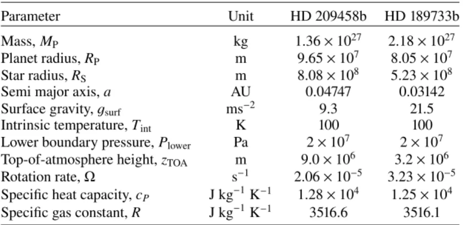
The atmospheric temperature on the 104 _{Pa isobar for the}

equilibrium simulations of both planets is shown in Fig.2. The thermal structure is qualitatively quite similar between the two planets, with a hot dayside and relatively much cooler nightside and a hotspot that is shifted eastward of the substellar point. HD 209458b is generally a few hundred Kelvin warmer than HD 189733b.

Figure3shows pressure-temperature profiles extracted from the 3D grid of equilibrium simulations of HD 209458b and HD 189733b, as well as dayside and nightside average profiles.

800

1000

1200

1400

1600

1800

2000

Temperature [K]

10

2

10

3

10

4

10

5

10

6

10

7

Pressure [Pa]

Equator

60◦ latitude Dayside average Nightside average Initial

600

800

1000

1200

1400

1600

1800

Temperature [K]

10

2

10

3

10

4

10

5

10

6

10

7

Pressure [Pa]

Equator 60◦ latitude Dayside average Nightside average Initial

Fig. 3.Pressure-temperature profiles extracted from the 3D grid of equi-librium simulations of HD 209458b (top) and HD 189733b (bottom). Solid grey lines show profiles at various longitude points around the equator (0◦

latitude) while dashed grey lines show profiles at various longitude points at a latitude of 60◦

. Area-weighted dayside average (red) and nightside average (blue) profiles are shown, along with the 1D radiative-convective equilibrium model profile used to initialise the 3D model (black).

The 1D radiative-convective equilibrium pressure-temperature profile used to initialise each 3D simulation is also shown. Both atmospheres have significant zonal temperature gradients for

P. 105 _{Pa with maximum day-night temperature contrasts of}

∼500 K. There is also a significant latitudinal thermal gradi-ent, at a given longitude and pressure, of several hundred Kelvin between the equator and mid-latitudes.

A high-pressure thermal inversion at P ∼ 106_{Pa is present in}

both equilibrium simulations. This is a result of the deep atmo-sphere slowly converging towards a temperature profile that is hotter than the 1D radiative-convective equilibrium profile used to initialise the model (shown in black in Fig. 3). Using a 2D steady-state circulation model,Tremblin et al.(2017) showed that the steady-state of the deep atmosphere is actually significantly hotter than predicted by 1D radiative-convective equilibrium models, likely due to the advection of potential temperature. It has also been noted that 3D simulations appear to slowly evolve towards hotter profiles in the deep atmosphere (Amundsen et al. 2016), however very long timescale simulations are required to actually reach the end state (as performed inSainsbury-Martinez

et al. 2019). Therefore, the results for pressures greater than ∼106Pa are likely to be strongly effected by the initial condition. The atmospheric circulation and thermal structure from the equilibrium simulations of HD 209458b and HD 189733b are almost identical to results presented in our previous work (Drummond et al. 2018a,b). Minor differences result from a number of changes in the model setup and chosen parameters, including, in no particular order: use of a different chemical equilibrium scheme (Gibbs energy minimisation versus analyt-ical chemanalyt-ical equilibrium formulae), slight adjustments to some planetary and stellar parameters (compare the parameters for

HD 209458b and HD 189733b in Table1 with those presented

inDrummond et al. 2018a,b, respectively), and the addition CO2

and HCN as opacity sources which were not previously included. Differences in the wind velocities and temperatures between the equilibrium and kinetics simulations due to chemical-radiative feedback are discussed later in Sect.3.3.

3.2. Chemical structure

To compare the differing chemical structure resulting from either the equilibrium or kinetics approach, we focus on each planet separately.

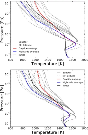
3.2.1. HD 209458b

Figure4shows the mole fractions of a subset of chemical species (CH4, CO, H2O, CO2, NH3, and HCN) on the P= 104 Pa

iso-bar for the equilibrium and kinetics simulations of HD 209458b. Figure5 shows both their equilibrium and kinetics abundances as vertical (pressure) mole fraction profiles at a series of equally spaced longitude points around the equator (i.e. at a latitude of θ= 0). We also show the vertical abundance profiles for a latitude of 45◦ _{in AppendixD. We show this particular subset}

of six molecules (out of a total of 30 species included in the chemical network) since each of these species are included as opacity sources in the model and they are also the six “species” for which the reduced chemical network was constructed (Venot et al. 2019).

The equilibrium abundances (left column of Fig.4) clearly trace the temperature structure (Fig. 2), as they necessarily should since the chemical equilibrium composition only depends on local pressure, temperature, and element abundances. The

abundances of CH4, CO2, and NH3 are lower on the warm

dayside compared with the cooler nightside. The equilibrium abundance of CH4is large enough in the coolest regions at this

pressure level to capture a significant number of carbon atoms, thereby reducing the equilibrium abundance of CO, though CO remains the dominant carbon species. The decrease in CO leads to a small increase in the equilibrium abundance of H2O as more

oxygen atoms are available. HCN shows a very small horizon-tal variation, since its abundance does not strongly depend on temperature for T > 1000 K (e.g.Heng & Tsai 2016). However, this molecule does show a significant vertical abundance gradi-ent (Fig.5). These trends are simply due to the temperature and pressure dependence of the Gibbs free energy of each chemical species. The equilibrium abundances of CH4, CO, and H2O are

almost identical to those presented inDrummond et al.(2018a), since the temperature structure is approximately the same.

We now focus on the differences in the chemical abun-dances between the equilibrium and kinetics simulations to investigate the effect of advection on the atmospheric

compo-sition. On the P = 104 Pa isobar the abundance fields from

45 90 135 180 225 270 315

Longitude [deg]

60

30

0

30

60

Latitude [deg]

1.2e-08

4.2e-08 1.5e-07 1.5e-07 5.1e-07 5.1e-07 1.8e-06 1.8e-06

CH

4

, equilibrium

10-9 10-8 10-7 10-6 10-5

Mole Fraction

45 90 135 180 225 270 315

Longitude [deg]

60

30

0

30

60

Latitude [deg]

7.6e-09

7.6e-09 1.9e-08 1.9e-08 4.7e-08 4.7e-08 1.1e-07 1.1e-07 2.8e-07 2.8e-07

CH

4

, kinetics

10-9 10-8 10-7 10-6 10-5

Mole Fraction

45 90 135 180 225 270 315

Longitude [deg]

60

30

0

30

60

Latitude [deg]

4.4e-04 4.4e-04 4.4e-04 4.4e-04 4.4e-04 4.4e-04 4.4e-04 4.4e-04

H

2

O, equilibrium

4.35e-04 4.36e-04 4.37e-04 4.38e-04 4.39e-04 4.40e-04 4.41e-04 4.42e-04 4.43e-04 4.44e-04

Mole Fraction

45 90 135 180 225 270 315

Longitude [deg]

60

30

0

30

60

Latitude [deg]

4.4e-04 4.4e-04 4.4e-04 4.4e-04 4.4e-04 4.4e-04 4.4e-04 4.4e-04 4.4e-04 _4.4e-04 4.4e-04 4.4e-04

H

2

O, kinetics

4.35e-04 4.36e-04 4.37e-04 4.38e-04 4.39e-04 4.40e-04 4.41e-04 4.42e-04 4.43e-04 4.44e-04

Mole Fraction

45 90 135 180 225 270 315

Longitude [deg]

60

30

0

30

60

Latitude [deg]

4.1e-08 4.1e-08 5.8e-08 5.8e-08 7.5e-08 7.5e-08 9.2e-08 9.2e-08 1.1e-07 1.1e-07

NH

3

, equilibrium

5.00e-08 1.00e-07 1.50e-07 2.00e-07 2.50e-07 3.00e-07 3.50e-07 4.00e-07 4.50e-07

Mole Fraction

45 90 135 180 225 270 315

Longitude [deg]

60

30

0

30

60

Latitude [deg]

1.3e-07

1.3e-07 1.8e-07 1.8e-07 2.4e-07 2.4e-07 2.9e-07 2.9e-07 3.5e-07 3.5e-07

NH

3

, kinetics

5.00e-08 1.00e-07 1.50e-07 2.00e-07 2.50e-07 3.00e-07 3.50e-07 4.00e-07 4.50e-07

Mole Fraction

Fig. 4.Mole fractions (colour scale and white contours) of CH4, H2O, NH3, CO, CO2 and HCN and wind vectors (arrows) on the 1 × 104Pa

(0.1 bar) isobar for the equilibrium simulation (left column) and the kinetics simulation (right column) of HD 209458b.

the equilibrium simulation for all of the presented species. The

kinetics abundances of CO and H2O become horizontally more

uniform compared with their equilibrium abundances, losing the variations across the cold, nightside mid-latitudes. The quan-titative differences between the two simulations, however, are

small and CO and H2O are the dominant carbon and oxygen

species throughout the atmosphere, as in the equilibrium case.

CO2 is close to its chemical equilibrium abundance for most

of the domain, on this pressure level, except in the coldest region (nightside mid-latitudes) where there is a small difference between the equilibrium and kinetics simulations. Here CO2 is

maintaining a “pseudo-equilibrium” with CO and H2O, since the

cycling between oxidised forms of carbon remains efficient (e.g.

Moses et al. 2011;Tsai et al. 2018). Therefore, CO2 only shows

an obvious difference with its chemical equilibrium value in the region where CO and H2O change, at the nightside mid-latitudes.

In other regions at this pressure level, the abundances of CO and H2O do not change significantly, and therefore neither does the

abundance of CO2.

The effect of advection on the horizontal abundance distri-bution of CH4at P= 104 Pa is more complex. The zonal

45 90 135 180 225 270 315

Longitude [deg]

60

30

0

30

60

Latitude [deg]

5.2e-04 5.2e-04 5.3e-04 5.3e-04 5.3e-04 5.3e-04 5.3e-04

5.3e-04

CO, equilibrium

5.21e-04 5.22e-04 5.23e-04 5.25e-04 5.27e-04 5.28e-04 5.30e-04 5.31e-04

Mole Fraction

45 90 135 180 225 270 315

Longitude [deg]

60

30

0

30

60

Latitude [deg]

5.3e-04 5.3e-04 5.3e-04 5.3e-04 5.3e-04 5.3e-04 5.3e-04 5.3e-04 5.3e-04 5.3e-04 5.3e-04 5.3e-04

CO, kinetics

5.21e-04 5.22e-04 5.23e-04 5.25e-04 5.27e-04 5.28e-04 5.30e-04 5.31e-04

Mole Fraction

45 90 135 180 225 270 315

Longitude [deg]

60

30

0

30

60

Latitude [deg]

1.5e-07 1.2e-07

1.5e-07 1.7e-07 1.7e-07 2.0e-07 2.0e-07 2.3e-07 2.3e-07

CO

2

, equilibrium

1.00e-07 1.25e-07 1.50e-07 1.75e-07 2.00e-07 2.25e-07 2.50e-07 2.75e-07

Mole Fraction

45 90 135 180 225 270 315

Longitude [deg]

60

30

0

30

60

Latitude [deg]

1.5e-07 1.2e-07

1.5e-07 1.8e-07 1.8e-07 1.8e-07 1.8e-07 2.1e-07 2.1e-07 2.4e-07 2.4e-07

CO

2

, kinetics

1.00e-07 1.25e-07 1.50e-07 1.75e-07 2.00e-07 2.25e-07 2.50e-07 2.75e-07

Mole Fraction

45 90 135 180 225 270 315

Longitude [deg]

60

30

0

30

60

Latitude [deg]

1.0e-09 1.0e-09 1.0e-09 1.0e-09 1.0e-09 1.0e-09 1.0e-09 1.0e-09 1.1e-09 1.1e-09

HCN, equilibrium

1e-09 2e-09 5e-09 1e-08 2e-08

Mole Fraction

45 90 135 180 225 270 315

Longitude [deg]

60

30

0

30

60

Latitude [deg]

4.5e-09 4.5e-09 6.0e-09 6.0e-09 7.9e-09 7.9e-09 1.0e-08 1.0e-08 1.4e-08 1.4e-08

HCN, kinetics

1.00e-09 2.00e-09 5.00e-09 1.00e-08 2.00e-08

Mole Fraction

Fig. 4.continued.

equilibrium simulation but there is a large latitudinal abundance gradient. The abundance of CH4from the kinetics simulation is

around an order of magnitude smaller in the equatorial region compared with at higher latitudes. A similar qualitative

struc-ture is found for NH3 and HCN, with lower abundances in the

equatorial region compared with higher latitudes.

From the vertical (pressure) profiles of the equatorial abun-dances of the six chemical species that we focus on here (Fig.5), it is clear that H2O and CO are the most abundant trace species

(i.e. after H2 and He), showing negligible abundance variations

with both pressure and longitude (for P > 106_{Pa). We note that}

the small variations in the abundances between the equilibrium

and kinetics simulations that are apparent in Fig.4 are mainly present at mid-latitudes and relatively small differences are also less apparent on the log-scale of this figure (Fig. 5). Both the kinetics abundances of NH3and HCN diverge from their

respec-tive equilibrium abundances between 105and 104Pa, with their abundances becoming zonally and vertically well mixed towards lower pressures.

The vertical profiles of the equatorial abundance of CH4are

the most interesting. In the pressure range 104−105_{Pa the}

kinet-ics abundances of CH4tend towards its equilibrium abundance in

the hottest part of the atmosphere. This has the effect of signif-icantly reducing the zonal abundance gradient, in this pressure

10

-12

₁₀

-11

₁₀

-10

₁₀

-9

₁₀

-8

₁₀

-7

₁₀

-6

₁₀

-5

₁₀

-4

₁₀

-3

Mole Fraction

10

2

10

3

10

4

10

5

10

6

10

7

Pressure [Pa]

CH

4 Equilibrium Kinetics

10

-5

₁₀

-4

₁₀

-3

Mole Fraction

10

2

10

3

10

4

10

5

10

6

10

7

Pressure [Pa]

CO

Equilibrium Kinetics

10

-5

₁₀

-4

₁₀

-3

Mole Fraction

10

2

10

3

10

4

10

5

10

6

10

7

Pressure [Pa]

H

2

O

Equilibrium Kinetics

10

-8

₁₀

-7

₁₀

-6

Mole Fraction

10

2

10

3

10

4

10

5

10

6

10

7

Pressure [Pa]

CO

2 Equilibrium Kinetics

10

-10

₁₀

-9

₁₀

-8

₁₀

-7

₁₀

-6

₁₀

-5

₁₀

-4

Mole Fraction

10

2

10

3

10

4

10

5

10

6

10

7

Pressure [Pa]

NH

3 Equilibrium Kinetics

10

-12

₁₀

-11

₁₀

-10

₁₀

-9

₁₀

-8

₁₀

-7

₁₀

-6

Mole Fraction

10

2

10

3

10

4

10

5

10

6

10

7

Pressure [Pa]

HCN

Equilibrium Kinetics

Fig. 5.Vertical mole fraction profiles for different longitude points around the equator, for the equilibrium simulation (dashed lines) and kinetics simulation (solid lines) of HD 209458b. Warmer colours indicate a profile that is closer to the substellar point, cooler colours are closer to the antistellar point.

range, by decreasing the nightside abundance. However, there remains a significant vertical abundance gradient in the same pressure range. This structure can be explained by CH4

under-going efficient zonal mixing in the pressure range 104−105Pa, while not being affected by vertical mixing. As a result, zonal abundance gradients are homogenised but vertical abundance gradients persist. For pressures less than 104 _{Pa the equatorial}

abundance of CH4becomes approximately vertically uniform.

CO2 is an interesting molecule in that it stays close to its

chemical equilibrium abundance for much of the equatorial region, except for the coolest nightside profiles at low pressures.

As previously discussed, CO2 maintains a pseudo-equilibrium

with CO and H2O, even once those molecules themselves have

quenched (Moses et al. 2011;Tsai et al. 2018). We attribute the departure of the abundances of CO2 from chemical equilibrium

as being due to its pseudo-equilibrium with CO and H2O, rather

than to quenching of CO2itself.

To understand the differences between the equilibrium and kinetics simulations, we compare the advection and chemical timescales. Where the advection timescale is much smaller than the chemical timescale (τadv << τchem) the composition should

much smaller than the advection timescale (τadv>> τchem), local

chemical equilibrium should hold. Where the two timescales are comparable (τadv ≈ τchem) both processes are important to

consider and the situation is more complex.

We estimate the zonal, meridional and vertical advection timescales as τu adv≈ 2πRP |u| , τ v adv≈ πRP 2|v|, and τ w adv≈ H |w|, respectively,

where RP is the planet radius, H is the vertical pressure scale

height and u, v, and w are the zonal, meridional, and vertical components of the wind velocity. We sample the wind velocities directly from the 3D grid to capture the spatial variation of the advection timescale. We note that these can be considered only as zeroth-order estimates.

We estimate the chemical timescale using the methods described inTsai et al.(2018). Since CH4 shows a particularly

interesting effect from advection, and because it is an important absorbing species, we focus on that molecule for this timescale comparison. However, we note that the chemical timescale, for a given pressure and temperature, varies significantly for different molecules (Tsai et al. 2018). The chemical timescale for CH4that

we use in this analysis has been specifically calculated for the

Venot et al.(2019) chemical network. In practice, we calculated the CH4chemical timescale for a grid of pressures and

tempera-tures. We then interpolated these timescales on to the model 3D grid using the pressure and temperature of each grid cell.

Figure 6 shows the ratio of the chemical to advection

timescales for CH4(α= τchem/τadv) for each of the three

com-ponents of the 3D wind (zonal, meridional, and vertical) for the kinetics simulation of HD 209458b. For the zonal component we show the timescales ratio as a function of pressure and longitude

for a meridional mean between ±30◦_{, whereas for the}

merid-ional and vertical components we show the timescales ratio as a function of pressure and latitude for a pole-to-pole slice cen-tred on the anti-stellar point (i.e. a longitude of φ= 0◦_{). Where}

α < 1 (red colours in Fig.6) the chemical timescale is smaller (faster) than the advection timescale and the chemical equilib-rium is expected to hold. However, where α > 1 (blue colours in Fig.6) the chemical timescale is larger (slower) than the advec-tion timescale and the atmosphere is expected to be well-mixed (in the direction of the considered wind velocity). We reiter-ate that both the chemical and advection timescales are only estimates, which conservatively should be seen as zeroth-order estimates.

For the zonal component of the timescale ratio (top panel, Fig.6), α decreases with increasing pressure, which is primarily due to the pressure and temperature dependence of the chemical timescale. Following the contour of α= 1, where the timescales are comparable, it is clear that there is a significant dependence of α on longitude. For a line of constant pressure, in between ∼103_{and ∼10}4_{Pa, α > 1 on the nightside whereas α < 1 for a}

significant portion of the dayside, largely due to the dependence of the chemical timescale on the local atmospheric temperature. This has the consequence that the atmosphere is expected to hold local chemical equilibrium on the dayside, but not on the night-side in the presence of zonal advection. This relates to the idea of “contamination” of the nightside by the chemistry of the dayside as discussed by previous authors (e.g.Agúndez et al. 2014a). The dayside atmosphere is hot enough to remain in chemical equi-librium and the fast zonal winds can transport this material to the cooler nightside that is not hot enough to maintain chemical equilibrium.

This structure of the timescale ratios helps to explain verti-cal profiles of the equatorial abundance of CH4 in Fig.5 (top

left panel) where we see its nightside abundances departing from chemical equilibrium and tending towards its equilibrium

50 100 150 200 250 300 350

Longitude [deg]

10

2

10

3

10

4

10

5

10

6

10

7

Pressure [Pa]

10-8 10-6 10-4 10-2 100 102 104 106 108

50

0

50

Latitude [deg]

10

2

10

3

10

4

10

5

10

6

10

7

Pressure [Pa]

10-8 10-6 10-4 10-2 100 102 104 106 108

50

0

50

Latitude [deg]

10

2

10

3

10

4

10

5

10

6

10

7

Pressure [Pa]

10-10 10-8 10-6 10-4 10-2 100 102 104 106 108 1010

Fig. 6. Ratios of the chemical to advection timescales for CH4

(α = τchem/τadv), for the zonal (top), meridional (middle), and

verti-cal (bottom) components of the wind for the kinetics simulation of

HD 209458b. We show a meridional-mean between ±30◦

latitude for the zonal component, and slices at a longitude of 0◦

(i.e. the antistel-lar point) for the meridional and vertical components. The colour scale shows α, with blue colours corresponding to α > 1 and red colours cor-responding to α < 1. The black contours show the α= 0.1, 1, 10 values. The fine structure shown in the plots is a reflection of regions where the wind velocity changes signs (e.g. eastward to westward) and the wind velocity approaches a value of zero over a very small region at the transition.

abundance in the hottest part of the dayside. Essentially this is horizontal quenching of CH4 (Agúndez et al. 2014a). We note

that the pressure range of this feature does not exactly match what we would expect from the timescale comparison shown in

Fig. 6. We attribute this simply to the fact that these timescale estimates are only zeroth-order estimates that we do not expect to precisely match the results of the full numerical simulations. We use the estimated timescales only as an aid to understand the complex 3D chemical structure that results from 3D advection.

For the meridional component of the timescale ratio (middle panel, Fig.6), the contour of α= 1 shows a significant latitudi-nal dependence and lies at lower pressures nearer to the equator. Again, this is primarily due to the temperature dependence of the chemical timescale. Near the equator the atmosphere is warmer, which results in a faster chemical timescale. The spatial varia-tion of the meridional wind velocity also plays a role. From this figure we can see that for some pressure range the atmosphere is expected to be in local chemical equilibrium in the equato-rial region, but not for higher-latitudes. This has the important consequence that, for some pressure levels, the equatorial region can become chemically isolated from the mid-latitudes and polar regions. This can explain why our results show different compo-sitions in the equatorial region compared with higher latitudes on the P= 104Pa isobar for CH4, and also for NH3, and HCN,

as shown in Fig.4.

The vertical component of the timescale ratio (bottom panel Fig. 6) is shown as a latitudinal slice at a longitude of 0◦. The structure of the vertical component of the timescale ratio is very similar to that of the meridional component. The con-tour of α = 1 lies at lower pressures in the equatorial region, where temperatures are higher, compared with higher latitudes. The transition lies at much lower pressures on the warmer day-side, in fact almost at the upper model boundary (see Fig.E.1). Because of this zonal variation in the ratio of the chemical to vertical advection timescale, we only expect vertical mixing to be important for the cooler nightside region. However, because the zonal advection timescale becomes faster than the chemical timescale at higher pressures, once a species becomes vertically homogenised on the nightside, that vertically quenched abun-dance can be subsequently transported zonally, leading to both horizontal and vertical homogenisation all around the planet. This explains the vertically uniform equatorial abundance of CH4shown in Fig.5.

3.2.2. HD 189733b

We now consider the simulations of the atmosphere of HD 189733b which, though overall cooler, shows a similar quali-tative thermal structure and circulation to HD 209458b. Figure7

(left column) shows the mole fractions of CH4, CO, H2O, CO2,

NH3, and HCN on the P = 104 Pa isobar for the equilibrium

simulation of HD 189733b. The distribution of abundances are generally very similar to those for the warmer HD 209458b (Fig. 7) but with quantitative differences due to differences in the temperature (Fig. 2). Since the atmosphere is cooler than HD 209458b there is an overall increased relative abundance

of CH4 by one to two orders of magnitude, which is favoured

thermodynamically for cooler temperatures. In particular, in the nightside mid-latitude regions the temperature is cold enough at P= 104Pa for CH4to become the most abundant carbon species,

replacing CO.

Figure7 (right column) shows the mole fractions of CH4,

CO, H2O, CO2, NH3, and HCN on the P= 104Pa isobar for the

kinetics simulation of HD 189733b. Here we see that for most molecules the effect of 3D advection is to largely remove the horizontal abundance gradients that are present in the chemi-cal equilibrium simulation. For CH4, CO, H2O, HCN, and NH3

the remaining horizontal abundance gradients are very small.

However, it is clear that CO2does not change significantly from

its chemical equilibrium abundance on the dayside. This means that temperature-dependent kinetics is still important for this molecule on the warm dayside and advection is not the domi-nant process in determining its abundance. Larger differences in the CO2 abundance between the equilibrium and kinetics

simu-lations are found on the cooler nightside. For CH4, CO, and H2O

our results qualitatively agree with our earlier work using a more simplified chemical scheme (Drummond et al. 2018a), as we also find that these molecules are efficiently horizontally mixed.

Figure 8 shows both the equilibrium and kinetics

abun-dances of CH4, CO, H2O, CO2, NH3, and HCN, as vertical

(pressure) mole fraction profiles around the equator. This also shows that most of the molecules are zonally and vertically well-mixed over a large pressure range at the equator. Compared with

HD 209458b (see Fig. 5), the molecules typically quench at

higher pressures, which is not surprising since the temperature is lower and the chemical timescale is longer.

The most obvious difference between our results for HD 189733b and HD 209458b are in the vertical profiles of CH4.

For HD 209458b, over a significant pressure range the abun-dance of CH4appears to be zonally but not vertically quenched,

with vertical mixing becoming important only for pressures

less than 104 _{Pa. For HD 189733b on the other hand we find}

that CH4 becomes vertically and horizontally well-mixed (i.e.

quenched) much deeper, approximately at the base of the equa-torial jet (Fig. 1). In the pressure range 105 Pa to 104 Pa the

equatorial abundance of CH4 becomes larger than any of its

equatorial equilibrium abundances, significantly increasing the relative abundance of CH4for this region of the atmosphere. This

structure is very similar to that found previously using a more simplified chemical scheme (Drummond et al. 2018a,b). In those earlier works we argued that this feature is due to meridional transport of material from the cooler mid-latitudes, where CH4

is more abundant at local chemical equilibrium, to the equatorial region.

In Drummond et al. (2018b) we conducted a simple tracer experiment that demonstrated that mass can be transported from the mid-latitudes into the equatorial region on a timescale of sev-eral hundred days. The tracer was initialised to an abundance of zero everywhere, except in a “source” region at high-pressure and high-latitudes. After several hundred days of model integra-tion, the tracer had increased in abundance significantly at the equator with a clear equator-ward transport occurring between 105 Pa and 103 Pa. Once the material is transported into the equatorial region, the material is rapidly distributed zonally and vertically by the fast equatorial jet and large dayside upwelling. Since the circulation for both HD 209458b and HD 189733b is broadly similar between this work and that tracer experiment, we expect the same transport process to be occuring. The difference between the two cases is in the chemical timescale, with a faster chemical timescale leading to a lower pressure quenching in the case of HD 209458b, above the region where the meridional transport is important.

The abundance profiles of CO2 are quite similar to those

found for HD 209458b. CO2remains close to its chemical

equi-librium value to much lower pressures than other molecules shown. For P > 103 _{Pa, we attribute the departure of the}

abun-dances of CO2 from chemical equilibrium as being due to its

pseudo-equilibrium with CO and H2O. But for P . 103 Pa,

where CO2 becomes approximately zonally uniform we expect

this to be due to zonal quenching of CO2itself.

Figure 9 shows the ratio of the chemical to advection

45 90 135 180 225 270 315

Longitude [deg]

60

30

0

30

60

Latitude [deg]

7.4e-07 2.4e-06 7.7e-06 2.5e-05 2.5e-05 8.0e-05 8.0e-05 8.0e-05 8.0e-05

CH

4

, equilibrium

10-7 10-6 10-5 10-4

Mole Fraction

45 90 135 180 225 270 315

Longitude [deg]

60

30

0

30

60

Latitude [deg]

3.1e-05 3.1e-05 3.3e-05 3.3e-05 3.6e-05 3.6e-05 3.9e-05 3.9e-05 4.2e-05 4.2e-05

CH

4

, kinetics

10-7 10-6 10-5 10-4

Mole Fraction

45 90 135 180 225 270 315

Longitude [deg]

60

30

0

30

60

Latitude [deg]

5.1e-04 5.1e-04 5.1e-04 5.1e-04 5.7e-04 _5.7e-04 5.7e-04 5.7e-04 6.2e-04 6.2e-04 6.2e-04 6.2e-04 6.8e-04 6.8e-04 7.4e-04 7.4e-04

H

2

O, equilibrium

4.50e-04 5.00e-04 5.50e-04 6.00e-04 6.50e-04 7.00e-04 7.50e-04 8.00e-04

Mole Fraction

45 90 135 180 225 270 315

Longitude [deg]

60

30

0

30

60

Latitude [deg]

4.7e-04 4.7e-04 4.7e-04 4.7e-04 4.7e-04 4.7e-04 4.7e-04 4.7e-04 4.8e-04 4.8e-04

H

2

O, kinetics

4.50e-04 5.00e-04 5.50e-04 6.00e-04 6.50e-04 7.00e-04 7.50e-04 8.00e-04

Mole Fraction

45 90 135 180 225 270 315

Longitude [deg]

60

30

0

30

60

Latitude [deg]

7.9e-08

1.1e-07 1.6e-07 2.2e-07 2.2e-07 2.2e-07 2.2e-07 3.2e-07 3.2e-07 3.2e-07 3.2e-07

NH

3

, equilibrium

1.00e-07 2.00e-07 5.00e-07 1.00e-06 2.00e-06 5.00e-06

Mole Fraction

45 90 135 180 225 270 315

Longitude [deg]

60

30

0

30

60

Latitude [deg]

2.8e-06 2.8e-06 2.9e-06 2.9e-06 2.9e-06 2.9e-06 3.0e-06 3.0e-06 3.1e-06 3.1e-06 3.1e-06

3.1e-06 3.1e-063.1e-06

NH

3

, kinetics

1.00e-07 2.00e-07 5.00e-07 1.00e-06 2.00e-06 5.00e-06

Mole Fraction

Fig. 7.Mole fractions (colour scale and white contours) of CH4, H2O, NH3, CO, CO2, and HCN and wind vectors (arrows) on the 1 × 104Pa

(0.1 bar) isobar for the equilibrium simulation (left column) and the kinetics simulation (right column) of HD 189733b.

Generally, the point at which the chemical and advection timescales become comparable (black line) lies at higher pres-sures than for HD 209458b. In addition, the pressure level at which the advection and chemical timescales become compara-ble is much more similar between the three components (zonal, meridional and vertical) compared with for HD 209458b, with the transition occurring at P ∼ 105_{Pa. Together this means that}

we expect the molecules to quench deeper, and for zonal, merid-ional and vertical quenching to act in approximately the same regions. This explains why we see such different behaviour for

CH4between HD 209458b and HD 189733b.

3.3. Chemical-radiative feedback

The advected chemical abundances of CH4, CO, CO2, H2O,

NH3, and HCN are used to calculate the total opacity in each

grid cell which is then used to calculate the radiative heat-ing rates. This allows for a chemical-radiative feedback process as changes in the chemical composition, due to the transport-induced quenching, can affect the thermal structure and circula-tion. Of course, the chemistry itself is strongly dependent on the temperature via the temperature-dependent rate coefficients.

Feedback between transport-induced quenching of chem-ical species and the temperature profile has previously