HAL Id: hal-00612491
https://hal.archives-ouvertes.fr/hal-00612491v2
Submitted on 2 May 2012
HAL is a multi-disciplinary open access
archive for the deposit and dissemination of
sci-entific research documents, whether they are
pub-lished or not. The documents may come from
teaching and research institutions in France or
abroad, or from public or private research centers.
L’archive ouverte pluridisciplinaire HAL, est
destinée au dépôt et à la diffusion de documents
scientifiques de niveau recherche, publiés ou non,
émanant des établissements d’enseignement et de
recherche français ou étrangers, des laboratoires
publics ou privés.
of SAR images with multinomial latent model
Koray Kayabol, Josiane Zerubia
To cite this version:
Koray Kayabol, Josiane Zerubia. Unsupervised amplitude and texture based classification of SAR
images with multinomial latent model. 2012. �hal-00612491v2�
a p p o r t
d e r e c h e r c h e
0249-6399
ISRN
INRIA/RR--7700--FR+ENG
Vision, Perception and Multimedia Understanding
Unsupervised amplitude and texture based
classification of SAR images with multinomial latent
model
Koray Kayabol — Josiane Zerubia
N° 7700 — version 2
Centre de recherche INRIA Sophia Antipolis – Méditerranée 2004, route des Lucioles, BP 93, 06902 Sophia Antipolis Cedex
classification of SAR images with multinomial
latent model
Koray Kayabol
∗, Josiane Zerubia
Theme : Vision, Perception and Multimedia Understanding Perception, Cognition, Interaction
´
Equipe-Projet Ariana
Rapport de recherche n° 7700 — version 2 — initial version July 2011 — revised version May 2012 — 29 pages
Abstract: We combine both amplitude and texture statistics of the Synthetic Aperture Radar (SAR) images for classification purpose. We use Nakagami density to model the class amplitudes and a non-Gaussian Markov Random Field (MRF) texture model with t-distributed regression error to model the textures of the classes. A non-stationary Multinomial Logistic (MnL) latent class label model is used as a mixture density to obtain spatially smooth class segments. The Classification Expectation-Maximization (CEM) algorithm is performed to estimate the class parameters and to classify the pixels. We resort to Integrated Classification Likelihood (ICL) criterion to determine the number of classes in the model. We obtained some classification results of water, land and urban areas in both supervised and unsupervised cases on TerraSAR-X, as well as COSMO-SkyMed data.
Key-words: High resolution SAR, TerraSAR-X, COSMO-SkyMed, classifica-tion, texture, multinomial logistic, Classification EM, Jensen-Shannon criterion
∗Koray Kayabol carried out this work during the tenure of an ERCIM ”Alain Bensoussan”
fond´
ee sur l’amplitude et la texture `
a l’aide
d’une mod`
ele multinomial latent
R´esum´e : Nous combinons les statistiques fond´ees sur l’amplitude et la texture d’images Radar `a Synth´ese d’Ouverture (RSO) `a des fins de classification. Nous utilisons la densit´e de Nakagami afin de mod´eliser les amplitudes des classes et un champ de Markov non-gaussien pour mod´eliser la texture, en utilisant l’erreur de r´egression t-distribu´ee afin de mod´eliser les textures des classes. Un mod´ele non-stationnaire Logistique Multinomial (LMn) d’´etiquettes de structure latente est utilis´e comme densit´e du m´elange afin d’obtenir des segments de classe liss´es spatialement. L’algorithme de Classification Esp´erance-Maximisation (CEM) est utilis´e pour estimer les param´etres des classes et classer les pixels. Nous avons recours au crit`ere ICV (Integrated Classification Vraisemblance) pour d´eterminer le nombre de classes dans le mod`ele. Nous avons obtenu des r´esultats de classification pour l’eau, les sols et les zones urbaines dans les cas supervis´e ou non-supervis´e sur des donn´ees TerraSAR-X ainsi que COSMO-SkyMed. Mots-cl´es : RSO haute r´esolution, TerraSAR-X, COSMO-SkyMed, classi-fication, texture, mod`ele logistique multinomial, Classification EM, crit´ere de Jensen-Shannon
Contents
1 Introduction 4
2 Multinomial Logistic Mixture of Amplitude and Texture
Den-sities 6
2.1 Class Amplitude and Texture Densities . . . 7
2.2 Mixture Density - Class Prior . . . 8
3 Classification EM Algorithm 8
4 Algorithm 11
4.1 Initialization . . . 12
4.2 Stopping Criterion . . . 12
4.3 Choosing the Number of Classes . . . 12
5 Simulation Results 13
1
Introduction
The aim of image classification is to assign each pixel of the image to a class with regard to a feature space. These features can be the basic image properties as in-tensity or amplitude. Moreover, some more advance abstract image descriptors as textures can also be exploited as feature. In remote sensing, image classifica-tion finds many applicaclassifica-tions varying from crop and forest classificaclassifica-tion to urban area extraction and epidemiological surveillance. Radar images are preferred in remote sensing because the acquisition of the images are not affected by light and weather conditions. First use of the radar images can be found in vegeta-tion classificavegeta-tion [2], [3] for instances. By the technological developments, we are now able to work with high resolution SAR images. The scope of this study is high resolution SAR image classification and we follow the model-based clas-sification approach. To model the statistics of SAR images, both empirical and theoretical probability density functions (pdfs) have been proposed [1]. Basic theoretical multi-look models are the Gamma and the Nakagami densities for intensity and amplitude images respectively. A recent review on the densities used in intensity and amplitude based modelling can be found in [4]. In this study, we work with SAR image amplitudes and consequently use the Nakagami density in model-based classification.
Finite Mixture Model (FMM) is a suitable statistical model to represent SAR image histogram and to perform a model-based classification [5]. One of the first uses of FMM in SAR image classification may be found in [6]. In [7] mixture of Gamma densities is used in SAR image processing. A combination of different probability density functions into a FMM has been used in [8] for medium resolution and in [9] for high resolution SAR images. In mixture mod-els, generally, a single model density is used to represent only one feature of the data, e.g. in SAR images, mixture of Gamma densities models the intensity of the images. To exploit different features in order to increase classification performance, we may combine different feature densities into a single classifier. There are some methods to combine the outcomes of the different and inde-pendent classifiers [32]. There are some feature selective mixture models [26], [27], [28] to combine different features in a FMM. In this study, rather than pixel-based mixture model, we use a block-based FMM which assembles both the SAR amplitudes and the texture statistics into a FMM simultaneously. In this approach, we factorize the block density using the Bayes rule in two parts which are 1) the amplitude density based on the central pixel of the block and 2) texture density based on the conditional density of the surrounding pixels given the central pixel.
Several texture models are used in image processing. We can list some of them as follows: Correlated K-distributed noise is used to capture the texture information of the SAR images in [10]. In [11], Gray Level Co-occurrence Matrix (GLCM) [15] and semivariogram [16] textural features are resorted to classify very high resolution SAR images (in particular urban areas). Markov Random Fields (MRFs) are proposed for texture representation and classification in [17] and [18]. A Gaussian MRF model which is a particular 2D Auto-Regressive (AR) model with Gaussian regression error is proposed for texture classifica-tion in [19]. MRF based texture models are used in optical and SAR aerial images for urban area extraction [20], [21], [22]. In [23] and [24], Gaussian AR texture model is resorted for radar image segmentation. In this study, we use
a non-Gaussian MRF model for texture representation. In this AR model, we assume that the regression error is an independent and identically distributed (iid) Student’s t-distribution. The t-distribution is a convenient model for ro-bust regression and it has been used in inverse problems in image processing [25], [29], [30] and image segmentation [31] as a robust statistical model.
The secondary target in land cover classification from SAR images is to find spatially connected and smooth class label maps. To obtain smooth and seg-mented class label maps, a post-processing can be applied to roughly classified pixels, but a Bayesian approach allows us to include smoothing constraints to classification problems. Potts-Markov image model is introduced in [33] for dis-crete intensity images. In [34] and [35], some Bayesian approaches are exploited for SAR image segmentation. Hidden Markov chains and random fields are used in [36] for radar image classification. [37] exploits a Potts-Markov model with MnL class densities in hyperspectral image segmentation. A double MRFs model is proposed in [23] for optical images to model the texture and the class labels as two different random fields. In [38], amplitude and texture characteris-tics are used in two successive and independent schemes for SAR multipolariza-tion image segmentamultipolariza-tion. In our spatial smoothness model, we assign a binary class map for each class which indicates the pixels belonging to that class. We introduce the spatial interaction within each binary map adopting multinomial logistic model [39]. In our logistic regression model, the probability of a pixel label is proportional to the linear combination of the surrounding binary pixels. If we compare the Potts-Markov image model [33] with ours, we may say that we have K different probability density functions for binary random fields of each class, instead of a single multi-level Gibbs distribution. The final density of the class labels is constituted by combining K probability densities into a multinomial density.
Defining a latent multinomial density function along with the amplitude and the texture models, we are able to incorporate both the class probabilities and the spatial smoothness into a single mixture model. Single models and algorithms may be preferred to avoid the propagation of the error between different models and algorithms.
Since our latent model is varying adaptively with respect to pixels, we ob-tain a non-stationary FMM. Non-stationary FMMs have been introduced for image classification in [40] and used for edge preserving image segmentation in [41], [42]. Using hidden MRFs model, a non-stationary latent class label model incorporated with finite mixture density is proposed in [43] for the segmentation of brain MR images. A non-stationary latent class label model is proposed in [44] by defining a Gaussian MRF over the parameters of the Dirichlet Com-pound Multinomial (DCM) mixture density and in [45] by defining a MRF over the mixture proportions. DCM density is also called multivariate Polya-Eggenberger density and the related process is called as Polya urn process [46], [47]. The Polya urn process is proposed to model the diffusion of a contagious disease over a population. The idea proposed in [46] has been already used in image segmentation [48] by assuming that each pixel label is related to an urn which contains all the neighbor labels of the central pixel. In this way, a non-parametric density estimation can be obtained for each pixel.
Besides the model-based classification approaches, there are also variational approaches proposed for optical [49], [50] and SAR image classification [51]. These level set approaches are based on the well-known Mumford-Shah [52]
for-malism in which the image pixels are fitted to a multilevel piecewise constant function while penalizing the length of the region boundaries [53]. These ap-proaches work well in the segmentation of the smooth images but may fail if the images contain some strong textures and noise.
Since we utilize a non-stationary FMM for SAR image classification, we re-sort to a kind of EM algorithm to fit the mixture model to the data. The EM algorithm [54], [55] and its stochastic versions [56] have been used for pa-rameter estimation in latent variable models. We use a computationally less expensive version of EM algorithm, namely Classification EM (CEM) [57], for both parameter estimation and classification, using the advantage of categorical random variables. In classification step, CEM uses the Winner-Take-All prin-ciple to allocate each data pixel to the related class according to the posterior probability of latent class label. After the classification step of CEM, we esti-mate the parameters of the class densities using only the pixels which belong to that class.
Determining the necessary number of classes to represent the data and ini-tialization are some drawbacks of the EM type algorithms. Running EM type algorithms several times for different model orders to determine the model order based on a criterion is a simple approach to reach a parsimonious solution. In [58], a combination of hierarchal agglomeration [59], EM and Bayesian Infor-mation Criterion (BIC) [60] is proposed to find necessary number of classes in the mixture model. [61] performs a similar strategy with Component-wise EM [62] and Minimum Message Length (MML) criterion [63, 64]. In this study, we combine hierarchical agglomeration, CEM and ICL [65, 66] criterion to get rid of the drawbacks of CEM.
In Section 2 and 3, the MnL mixture model and CEM algorithm are given. The simulation results are shown in Section 5. Section 6 presents the conclusion and future work.
2
Multinomial Logistic Mixture of Amplitude
and Texture Densities
We assume that the observed amplitude sn ∈ R+ at the nth pixel, where n ∈
R = {1, 2, . . . , N } represents the lexicographically ordered pixel index, is free
from any noise and instrumental degradation. We denote s to be the vector representation of the entire image and sn to be the vector representation of the
d × d image block located at nth pixel. Every pixel in the image has a latent
class label. Denoting by K the number of classes, we encode the class label as a K dimensional categorical vector zn whose elements zn,k, k ∈ {1, 2, . . . , K}
have the following properties: 1) zn,k ∈ {0, 1} and 2)
PK
k=1zn,k = 1. We may
write the probability of snas the marginalization of the joint probability density
p(sn, zn|Θ, πn) = p(sn|zn, Θ)p(zn|πn), [5], as p(sn|Θ) = X zn p(sn|zn, Θ)p(zn|πn) = X zn K Y k=1 [p(sn|θk)πn,k]zn,k (1)
where πn,k = p(zn,k = 1) represent the mixture proportions and ensure that
PK
k=0πn,k = 1. θkare the parameters of the class densities and Θ = {θ1, . . . , θK}
is the set of the parameters. By taking into consideration that zn is a
cate-gorical random vector distributed as a multinomial, and assuming that πn =
{πn,1, . . . , πn,K} is spatially invariant, (1) is reduced to classical FMM as follow
p(sn|Θ) = K
X
k=1
p(sn|θk)πn,k (2)
We prefer to use the notation in (1) to show the contribution of the multinomial density of class label, p(zn), into finite mixture model more explicitly. We give
the details of the class and the mixture densities in the following two sections.
2.1
Class Amplitude and Texture Densities
Our aim is to use the amplitude and the texture statistics together to classify the SAR images. We may write the density of an image block as a joint density of the central pixel and the surrounding pixels as p(sn|θk) = p(sn, s∂n|θk). Using
Bayes rule, we factorize the density of the image block as
p(sn|θk) = pA(sn|θk)pT(s∂n|sn, θk) (3)
In this last expression, the first and the second terms represent the amplitude and the texture densities.
We model the class amplitudes using Nakagami density, which is a basic theoretical multi-look amplitude model for SAR images [1]. We express the class amplitude density as
pA(sn|µk, νk) = 2 Γ(νk) µ νk µk ¶νk s2νk−1 n e ³ −νks2µkn ´ . (4)
We introduce a t-MRF texture model to use the contextual information for classification. We write the t-MRF texture model using the neighbors of the pixel in N (n)
sn=
X
n0∈N (n)
αk,n0sn0+ tk,n (5)
where αk,n0 is the regression coefficient and the regression error tk,n is an iid
t-distributed zero-mean random variable with degree of freedom parameter βk
and scale parameters δk. In this way, we may write the class texture density as
a t-distribution such that
pT(s∂n|sn, αk, βk, δk) = Γ((1 + βk)/2) Γ(βk/2)(πβkδk)1/2 · 1 +(sn− s T ∂nαk)2 βkδk ¸−βk+12 (6)
where the vector αkcontains the regression coefficients αk,n0. The t-distribution
can also be written in implicit form using both of a Gaussian and a Gamma densities [71] p(s∂n|sn, αk, βk, δk) = Z p(s∂n|sn, αk, τn,k, δk)p(τn,k|βk)dτn,k = Z N µ sn ¯ ¯ ¯ ¯sT∂nαk, δk τn,k ¶ G µ τn,k ¯ ¯ ¯ ¯β2k,β2k ¶ dτn,k. (7)
We use the representation in (7) for calculation of the parameters using EM method nested in CEM algorithm.
2.2
Mixture Density - Class Prior
The prior density p(zn|πn) of the categorical random variable zn is naturally
an iid multinomial density with parameters πn as introduced in (1) as
p(zn|πn) = Mult(zn|πn) = K Y k=1 πzn,k n,k (8)
We are not able to obtain a smooth class label map if we use an iid multi-nomial. We need to use a density which models the spatial smoothness of the class labels. We can define a prior on πn to introduce the spatial interaction.
If we define a conjugate Dirichlet prior on πn and integrate out πn from the
model, we reach the DCM density [48]. The DCM density is the density of the Polya urn process and gives us a non-parametric density estimation in a defined window. In case that the estimated probabilities are almost equal in that win-dow, Polya urn model may fail to make a decision to classify the pixels. [44] proposes a MRF model over the spatially varying parameter of DCM density. We use a contrast function called Logistic function [39] which emphasizes the high probabilities while attenuating the low ones. The logistic function allows us to make an easier decision by discriminating the probabilities closed to each other.
We can introduce the spatial interactions of the categorical random field by defining a binary spatial auto-regression model for each binary class map (or mask). Consequently, the probability density function of this multiple binary class maps model is a Multinomial Logistic. If we substitute the logistic model with parameter η in place of πn,k, we obtain MnL density for the problem at
hand as p(zn|Z∂n, η) = K Y k=1 Ã exp(ηvk(zn,k)) PK j=1exp(ηvj(zn,j)) !zn,k (9) where vk(zn,k) = 1 + X m∈M(n) zm,k. (10)
and Z∂n = {zm : m ∈ M(n), m 6= n} is the set which contains the neighbors
of zn in a window M(n) defined around n. The function vk(zn,k) returns the
number of labels which belong to class k in a given window. The mixture density in (9) is spatially-varying with given function vk(zn,k) in (10).
3
Classification EM Algorithm
Since our purpose is to cluster the observed image pixels by maximizing the marginal likelihood given in (1) such as
{ ˆΘ, ˆη} = max {Θ,η} N Y n=1 X zn p(sn|zn, Θ)p(zn|Z∂n, η) (11)
we use an EM type algorithm to deal with the summation. The EM log-likelihood function is written as
QEM(Θ|Θt−1) = N X n=1 K X k=1 log{p(sn|zn,k, θk)p(zn,k|Z∂n, η)}p(zn,k|sn, Z∂n, Θt−1) (12) where θk = {αk, βk, δk, µk, νk} and Θ = {θ1, . . . , θK, η}.
If we used the exact EM algorithm to find the maximum of Q(Θ|Θt−1) with
respect to Θ, we would need to maximize the parameters for each class given the expected value of the class labels. Instead of this, we use the advantage of working with categorical random variables and resort to Classification EM algorithm [57]. We can partition the pixel domain R into K non-overlapped regions such that R = SKk=1Rk and Rk
T
Rl = 0, k 6= l. We can write the
classification log-likelihood function as
QCEM(Θ|Θt−1) = K X k=1 X m∈Rk log{p(sm|zm,k, θk)p(zm,k|Z∂m, η)}p(zm,k|sn, Z∂n, Θt−1) (13)
The CEM algorithm incorporates a classification step between the E-step and the M-step which performs a simple Maximum-a-Posteriori (MAP) estimation to find the highest probability class label. Since the posterior p(zn,k|sn, Z∂n, Θt−1)
is a discrete probability density function of a finite number of classes, we can perform the MAP estimation by choosing the maximum class probability. We summarize the CEM algorithm for our problem as follows:
E-step: For k = 1, . . . , K and n = 1, . . . , N , calculate the posterior proba-bilities p(zn,k|sn, Z∂n, Θt−1) = p(sn|θkt−1)zn,k exp(η t−1v k(zn,k)) PK j=1exp(ηt−1vj(zn,j)) (14)
given the previously estimated parameter set Θt−1 using (4), (6) and (3).
C-step: For n = 1, . . . , N , classify the nth pixel into class j as zn,j = 1
by choosing j which maximizes the posterior p(zn,k|sn, Z∂n, Θt−1) over k =
1, . . . , K as
j = arg max
k p(zn,k|sn, Z∂n, Θ
t−1) (15)
M-step: To find a Bayesian estimate, maximize the classification log-likelihood in (13) and the log-prior functions log p(Θ) together with respect to Θ as
Θt−1= arg max
Θ {QCEM(Θ|Θ
t−1) + log p(Θ)} (16)
To maximize this function, we alternate among the variables µk, νk, αk,
βk and δk. We only define an inverse Gamma prior with mean 1 for βk ∼
IG(βk|Nk, Nk) where Nk is the number of pixels in class k. We choose this prior
among some positive densities by testing their performance in the simulations. We have obtained better results with small values of βk. This prior ensures βk
to take a value around 1. We assume uniform priors for the other parameters. The functions of the amplitude parameters over all pixels are written as follows
Q(µk; Θt−1) = −Nkνklog µk− νk µk X n∈Rk s2 n (17) Q(νk; Θt−1) = Nkνklogµνkk − Nklog Γ(νk)+ (2νk− 1) P n∈Rklog sn− νk µk P n∈Rks 2 n (18)
We estimate the texture parameters using another sub-EM algorithm nested within CEM. The nested EM algorithm has already been studied in [70]. We can express the t-distribution as a Gaussian scale mixture of gamma distributed la-tent variables τn,k. Thereby, the EM log-likelihood functions of the t-distribution
in (6) are written as [71], [30] Q(αk; Θt−1) = − X n∈Rk (sn− sT∂nαk)2 2δk hτn,ki (19) Q(δk; Θt−1) = −Nk 2 log δk− X n∈Rk (sn− sT∂nαk)2 2δk hτn,ki (20) Q(βk; Θt−1) = −Nklog Γ(βk 2 ) + Nkβk 2 log βk 2 − Nk βk − X n∈Rk hτn,kiβk 2 µ 1 + (sn− s T ∂nαk)2 2δkβk ¶ + X n∈Rk µ βk 2 ¶ hlog τn,ki − (Nk+ 1) log βk (21)
where hτn,ki is the posterior expectation of the gamma distributed latent
vari-able and calculated as
hτn,ki =βk+ 1 βk µ 1 +(sn− s T ∂nαk)2 βkδk ¶−1 (22)
For simplicity, we use h.i to represent the posterior expectation h.iτn,k|Θt−1.
The solutions to (17), (19) and (20) can be easily found as
µk = 1 Nk Nk X n=1 s2 n (23) αk = (ST∂S∂)−1ST∂s (24) δk= Nk X n=1 (sn− φTnαk)2 Nk hτn,ki (25)
where S∂ is N × d2− 1 matrix whose columns are s∂n’s. For (18) and (21),
we use a zero finding method to determine their maximum [72] by setting their first derivatives to zero
log νk µk − ψ1(νk) + 2 Nk Nk X n=1 log sn= 0 (26)
logβk 2 − ψ1( βk 2 ) + 1 + 1 Nk Nk X n=1 hlog τn,ki − hτn,ki − Nk+ 1 βk + Nk β2 k = 0 (27)
The parameter η of the MnL class label is found by maximizing the following function Q(η; Θt−1) = N X n=1 ηvk(zn,k) − log K X j=1 eηvj(zn,j) (28)
We use a Newton-Raphson iteration to fit η as
ηt= ηt−1−1
2
∇Q(η; Θt−1)
∇2Q(η; Θt−1) (29)
where the operators ∇· and ∇2· represent the gradient and the Laplacian of the
function with respect to η.
4
Algorithm
In this section, we present the details of the unsupervised classification algo-rithm. Our strategy follows the same general philosophy as the one proposed in [59] and developed for mixture model in [58, 61]. We start the CEM algorithm with a large number of classes, K = Kmax, and then we reduce the number of
classes to K ← K − 1 by merging the weakest class in probability to the one that is most similar to it with respect to a distance measure. The weakest class may be found using the average probabilities of each class as
kweak= arg min k 1 Nk X n∈Rk p(zn,k|sn, Z∂n, Θt−1) (30)
Kullback-Leibler (KL) type divergence criterions are used in hierarchical texture segmentation for region merging [73]. We use a symmetric KL type dis-tance measure called Jensen-Shannon divergence [74] which is defined between two probability density functions, i.e. pkweak and pk, k 6= kweak, as
DJS(k) =1
2DKL(pkweak||q) +
1
2DKL(pk||q) (31) where q = 0.5pkweak+ 0.5pk and
DKL(p||q) =
X
k
p(k) logp(k)
q(k) (32)
We find the closest class to kweak as
l = arg min
k DJS(k) (33)
and merge these two classes to constitute a new class Rl← Rl
S
Rkweak.
We repeat this procedure until we reach the predefined minimum number of classes Kmin. We determine the necessary number of classes by observing the
ICL criterion explained in Section 4.3. The details of the initialization and the stopping criterion of the algorithm are presented in Section 4.1 and 4.2. The summary of the algorithm can be found in Table 1
Table 1: Unsupervised CEM algorithm for classification of amplitude and tex-ture based mixtex-ture model.
Initialize the classes defined in Section 4.1 for K = Kmax.
While K ≥ Kmin, do η = c, c ≥ 0
While the number of changes > N × 10−3, do
E-step: Calculate the posteriors in (14) C-step: Classify the pixels regarding to (15)
M-step: Estimate the parameters of amplitude and tex-ture densities using (22-27)
Update the smoothness parameter η using (29) Find the weakest class using (30)
Find the closest class to the weakest class using (31-33) Merge these two classes Rl← Rl
S
Rkweak
K ← K − 1
4.1
Initialization
The algorithm can be initialized by determining the class areas manually in case that there are a few number of classes. We suggest to use an initialization strat-egy for completely unsupervised classification. It removes the user intervention from the algorithm and enables to use the algorithm in case of large number of classes. First, we run the CEM algorithm for one global class. Using the cumulative distribution of the fitted Nakagami density g = FA(sn|µ0, ν0) where
g ∈ [0, 1] and dividing [0, 1] into K equal bins, we can find our initial class
parameters as µk = FA−1(gk|µ0, ν0), k = 1, . . . , K where gk’s are the centers of
the bins. We initialize the other parameters using the estimated parameters of the global class. We reset the parameter η to a constant c after reducing the number of classes.
4.2
Stopping Criterion
We observe the number of changes in the updated pixel labels after classification step to decide the convergence of the CEM algorithms. If the number of change is less then a threshold, i.e. N × 10−3, the CEM algorithm is stopped.
4.3
Choosing the Number of Classes
The SAR images which we used have a small number of classes. We aim at validating our assumption on small number of classes using the Integrated Clas-sification Likelihood (ICL) [66]. Even though BIC is the most used and the most practical criterion for large data sets, we prefer to use ICL because it is developed specifically for classification likelihood problem, [65], and we have obtained better results than BIC in the determination of the number of classes.
In our problem, the ICL criterion may be written as ICL(K) = N X n=1 K X k=1 log{p(sn|ˆθk)zˆn,kp(ˆzn,k|ˆZ∂n, ˆη)} −1 2dKlog N + P (K) (34) where dK is the number of free parameters. In our case, it is dK = 12 ∗ K + 1.
The term P (K) is formed by the logarithm of the prior distribution of the parameters. In our case, it is P (K) = PKk=1log IG( ˆβk|Nk, Nk). We also use
the BIC criterion for comparison. It can be written as
BIC(K) = N X n=1 log ÃK X k=1 p(sn|ˆθk)p(zn,k|Z∂n, ˆη) ! −1 2dKlog N + P (K) (35)
5
Simulation Results
This section presents the high resolution SAR image classification results of the proposed method called ATML-CEM (Amplitude and Texture density mixtures of MnL with CEM), compared to the corresponding results obtained with other methods. The competitors are Dictionary-based Stochastic EM (DSEM) [9], Copulas-based DSEM with GLCM (CoDSEM-GLCM) [11], Multiphase Level Set (MLS) [67], [68] and K-MnL. We have also tested three different versions of ATML-CEM method. One of them is supervised ATML-CEM [69] where training and testing sets are determined by selecting some spatially disjoint class regions in the image, and we run the algorithm twice for training and testing. We implement the other two versions by considering only Amplitude (AML-CEM) or only Texture (TML-CEM) statistics.
MLS method is based on the piecewise constant multiphase Chan-Vese model [53] and implemented by [67], [68]. In this method, we set the smoothness parameter to 2000 and step size to 0.0002 for all data sets. We tune the number of iteration to reach the best result. The K-MnL method is the sequential combination of K-means clustering for classification and Multinomial Logistic label model for segmentation to obtain a more fair comparison with K-means clustering since K-means does not provide a segmented map. The weak point of the K-means algorithm is that it does not converge to the same solution every time, since it starts with random seed. Therefore, we run the K-MnL method 20 times and select the best result among them.
We tested the algorithms on the following four SAR image patches:
SYN: 200 × 200 pixels, synthetic image constituted by collating 4 different 100 × 100 patches from TSX1 image. The small patches are taken from water, urban, land and forest areas (see Fig. 2(a)).
TSX1: 1200 × 1000 pixels, HH polarized TerraSAR-X Stripmap (6.5 m ground resolution) 2.66-look geocorrected image which was acquired over Sanchagang, China (see Fig. 4(a)). ©Infoterra.
TSX2: 900 × 600 pixels, HH polarized, TerraSAR-X SpotLight (8.2 m ground resolution) 4-look image which was acquired over the city of Rosen-heim in Germany (see Fig. 6(a)). ©Infoterra.
Table 2: Accuracy (in %) of the supervised (S), semi-supervised (Ss) and unsu-pervised (U) classification of SYN image for 4 classes and in average.
water urban trees land average ATML-CEM (S) 99.02 99.46 99.28 99.30 99.27 K-MnL (Ss) 96.58 80.18 99.60 90.32 91.92 MLS (Ss) 100.00 60.46 1.13 42.55 51.03 AML-CEM (U) 97.53 97.89 97.72 94.57 96.93 TML-CEM (U) 98.18 81.10 85.79 88.72 88.45 ATML-CEM (U) 97.74 97.61 97.73 94.81 96.97
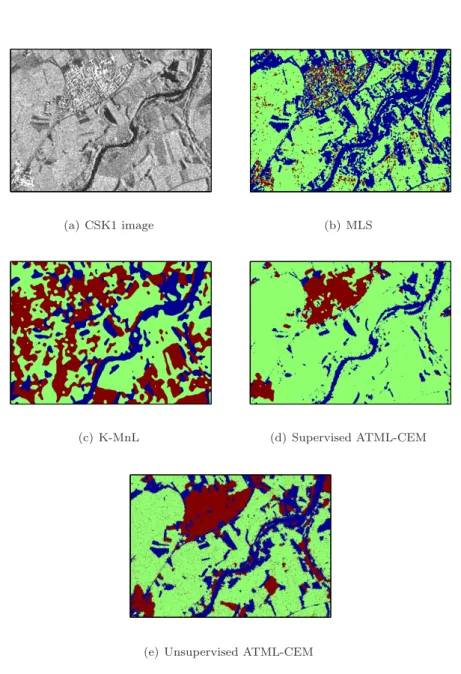
CSK1: 672 × 947 pixels, HH polarized COSMO-SkyMed Stripmap (2.5 m ground resolution) single-look image which was acquired over Lombriasco, Italy (see Fig. 9(a)). ©ASI.
For all real SAR images (TSX1, TSX2 and CSK1) classified by ATML-CEM versions, we use the same setting for model and initialization. The sizes of the windows for texture and label models are selected to be 3×3 and 13×13 respectively by trial and error. For synthetic SAR image (SYN), we utilize a 21×21 window in MnL label model and a 3×3 window in texture model. We initialize the algorithm as described in Section 4.1 and estimate all the parameters along the iterations.
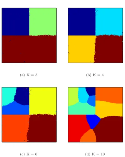
We produce SYN image to test the performance of the unsupervised ATML-CEM algorithm in the estimation of the number of classes, because the real images may contain more classes than our expectations and choosing different classes by eyes to construct a ground-truth is very hard if the number of classes is high. From Fig. 1(a), we can see that the ICL and BIC plots have their first peaks at 4. The outcomes of the algorithm for different number of classes can be seen in Fig. 3. The numerical results are listed in Table 2. For supervised case, we allocate 25% of the data for training and 75% for testing. The similar results of AML-CEM and ATML-CEM show that the contribution of texture information is very weak in this data set. From Fig. 2, we can see that the classification map of ATML-CEM is obviously better than those of K-MnL, MLS and TML-CEM.
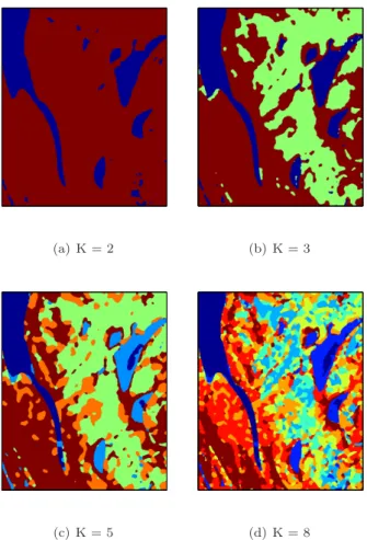
For TSX1 image in Fig.4(a), the full ground-truth map (Courtesy of V. Krylov) is manually generated. Fig.4 shows the classification results where the red colored regions indicate the misclassified parts according to 3-classes ground-truth map. We can see the plotted ICL and BIC values with respect to the number of classes in Fig. 1(b). The plots are increasing, but the in-crements in both ICL and BIC start to slow down at 3. Fig. 5 shows several classification maps found for different numbers of classes. Since we have the 3-classes ground-truth map, we compare our results numerically in the 3-classes case. The numerical accuracy results are given in Table 3. While supervised ATML-CEM gives the better result in average, unsupervised ATML-CEM and supervised DSEM-MRF follow it. Among the semi-supervised and unsupervised methods, the performance of ATML-CEM is better than the others in average, but results of K-MnL and AML-CEM are close to its results.
From the experiment with TSX1 image, we realize that if the image does not have strong texture, we cannot benefit from including texture statistics into the model. To reveal the advantage of using texture model, we exploit the
ATML-1 2 3 4 5 6 7 8 9 10 −10.5 −10 −9.5 −9 −8.5 −8 −7.5 −7x 10 4 Number of classes ICL BIC (a) SYN 1 2 3 4 5 6 7 8 −4 −3.9 −3.8 −3.7 −3.6 −3.5 −3.4 −3.3 −3.2x 10 6 Number of classes ICL BIC (b) TSX1 1 2 3 4 5 6 7 8 9 10 11 12 13 14 15 −2.16 −2.14 −2.12 −2.1 −2.08 −2.06 −2.04 −2.02 −2 −1.98x 10 6 Number of classes ICL BIC (c) TSX2 1 2 3 4 5 6 7 8 9 10 11 12 −3.1 −3 −2.9 −2.8 −2.7 −2.6 −2.5x 10 6 Number of classes ICL BIC (d) CSK1
Figure 1: ICL and BIC values of the classified (a) SYN (b) TSX1, (c) TSX2 and (d) CSK1 images for several numbers of sources.
Table 3: Accuracy (in %) of the supervised (S), semi-supervised (Ss) and unsu-pervised (U) classification of TSX1 image in water, wet soil and dry soil areas and average.
water wet soil dry soil average
DSEM-MRF (S) 90.00 69.93 91.28 83.74 ATML-CEM (S) 89.88 76.38 87.33 84.53 K-MnL (Ss) 89.71 86.13 72.42 82.92 MLS (Ss) 87.90 66.19 42.48 65.53 AML-CEM (U) 88.24 62.99 96.39 82.54 TML-CEM (U) 51.61 65.89 91.90 69.80 ATML-CEM (U) 87.93 65.58 95.55 83.02
CEM algorithm for urban area extraction problem on TSX2 image in Fig. 6(a). Table 4 lists the accuracy of the classification in water, urban and land areas and average according to a groundtruth class map (Courtesy of A. Voisin). We include the result of CoDSEM-GLCM [11] which is the extended version of the DSEM method by including texture information. In both supervised and unsupervised cases, ATML-CEM provides better results than the others. The combination of the amplitude and the texture features helps to increase the
(a) SYN image (b) K-MnL
(c) MLS (d) Supervised ATML-CEM
(e) Unsupervised ATML-CEM
Figure 2: (a) SYN image, (b), (c) and (d) classification maps obtained by K-MnL, MLS, supervised and unsupervised ATML-CEM methods. Dark blue, light blue, yellow and red colors represent class 1 (water), class 2 (urban), class 3 (trees) and class 4 (land), respectively.
(a) K = 3 (b) K = 4
(c) K = 6 (d) K = 10
Figure 3: Classification maps of SYN image obtained with unsupervised ATML-CEM method for different numbers of classes K = {3,4,5,10}.
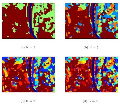
quality of classification in average. From Fig. 6, we can see that the MLS and K-MnL methods fail to classify the urban areas. MLS provides a noisy classification map. The classification map of ATML-CEM agglomerates the tree and hill areas into urban area, since their textures are more similar to urban texture than the others. Misclassification in water areas is caused by the dark shadowed regions. Fig. 1(c) shows the ICL and BIC values. From this plot, we can see that the necessary number of classes should be 3, since both plots are saturated after 3. Fig. 7 presents the classification maps for 3-, 5-, 7-and 12-classes cases.
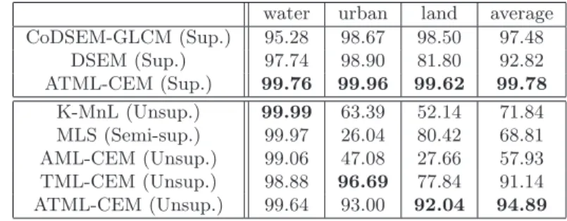
We have tested ATML-CEM on another patch called CSK1 (see Fig. 9(a)). Tab. 5 lists the numerical results. Among the supervised methods, ATML-CEM is very successful. Since this SAR image is a single-look observation, the noise level is higher than in the other images. We can obtain some good unsupervised classification results after applying a denoising process. Among the Lee, Frost and Wiener filters, we prefer using a 2D adaptive Wiener filter with 3 × 3 window proposed in [75], because we obtain better classification results. In Fig. 8, we show the histogram of the intensity of the CSK1 image before and after
(a) TSX1 image (b) MLS
(c) K-MnL (d) Supervised ATML-CEM
(e) Unsupervised ATML-CEM
Figure 4: (a) TSX1 image, (b), (c) and (d) classification maps obtained by K-MnL, MLS, supervised and unsupervised ATML-CEM methods. Dark blue, light blue, yellow and red colors represent water, wet soil, dry soil and misclas-sified areas, respectively.
(a) K = 2 (b) K = 3
(c) K = 5 (d) K = 8
Figure 5: Classification maps of TSX1 image obtained with unsupervised ATML-CEM method for different numbers of classes K = {2,3,5,8}.
Table 4: Accuracy (in %) of the supervised (S), semi-supervised (Ss) and unsu-pervised (U) classification of TSX2 image in water, urban and land areas and overall.
water urban land average CoDSEM-GLCM (S) 91.28 98.82 93.53 94.54 DSEM (S) 92.95 98.32 81.33 90.87 ATML-CEM (S) 98.60 97.56 94.78 96.98 K-MnL (Ss) 100.00 79.03 80.33 86.45 MLS (Ss) 89.47 35.62 84.71 69.93 AML-CEM (U) 92.36 98.29 80.97 90.54 TML-CEM (U) 89.88 96.18 72.32 86.12 ATML-CEM (U) 94.17 98.76 80.93 91.29
denoising to justify that our Nakagami/Gamma density assumption is still valid after denoising. CSK1 is an 8-bits image and we plot its intensity histogram between 0 and 254 to demonstrate two histograms in a comparable case.
ATML-(a) TSX 1 (b) MLS
(c) K-MnL (d) Supervised ATML-CEM
(e) Unsupervised ATML-CEM
Figure 6: (a) TSX2 image, (b), (c) and (d) classification maps obtained by K-MnL, MLS, supervised ATML-CEM and unsupervised ATML-CEM methods. Blue, red and green colors represent water, urban and land areas, respectively.
CEM provides significantly better results in overall, see Fig. 9 and Table 5. The results in Fig. 9 are found for 3-classes case, since we have the 3-classes ground-truth map. The optimum number of classes is found as 5 according to ICL criterion, see Fig. 1(d). Fig. 10 shows some classification maps for different numbers of classes.
The simulations were performed on MATLAB platform on a PC with Intel Xeon, Core 8, 2.40 GHz CPU. The number of iterations and total required time in minutes for the algorithm are shown in Table 6. We also present the required time in seconds for a single iteration in case of the number of classes
(a) K = 3 (b) K = 5
(c) K = 7 (d) K = 15
Figure 7: Classification maps of TSX2 image obtained with unsupervised ATML-CEM method for different numbers of classes K = {3,5,7,12}.
0 50 100 150 200 250 0 1000 2000 3000 4000 5000 6000
(a) Histogram before denoising
0 50 100 150 200 250 0 1000 2000 3000 4000 5000 6000
(b) Histogram after denoising
Figure 8: Histograms of the intensity of the CSK1 image (a) before and (b) after denoising.
K = {3, 6, 9, 12}. The algorithm reaches a solution in a reasonable time, if we
Table 5: Accuracy (in %) of the supervised (S), semi-supervised (Ss) and unsu-pervised (U) classification of CSK1 image in water, urban and land areas and overall. Note that unsupervised classification results are obtained after denois-ing.
water urban land average CoDSEM-GLCM (Sup.) 95.28 98.67 98.50 97.48 DSEM (Sup.) 97.74 98.90 81.80 92.82 ATML-CEM (Sup.) 99.76 99.96 99.62 99.78 K-MnL (Unsup.) 99.99 63.39 52.14 71.84 MLS (Semi-sup.) 99.97 26.04 80.42 68.81 AML-CEM (Unsup.) 99.06 47.08 27.66 57.93 TML-CEM (Unsup.) 98.88 96.69 77.84 91.14 ATML-CEM (Unsup.) 99.64 93.00 92.04 94.89
Table 6: The number of pixels of TSX1, TSX2 and CSK1; Corresponding re-quired time in seconds for a single iteration in case of K = {2, 4, 6, 8}; Total required time in minutes; and Total number of iterations.
# of pixels K = 8 K = 6 K = 4 K = 2 Total [min.] Total it.
TSX1 1200e+3 7.04 6.18 4.62 3.55 5.07 57
TSX2 540e+3 2.83 2.31 1.89 1.58 3.97 110
CSK1 636e+3 3.52 3.42 2.65 2.13 2.42 50
6
Conclusion and Future Work
We have proposed a Bayesian model which uses amplitude and texture features together in a FMM along with nonstationary latent class labels. Using these two features together in the model, we obtain better high resolution SAR image classification results, especially in the urban areas.
Furthermore, using an agglomerative type unsupervised classification method, we eliminate the negative effect of the latent class label initialization. According to our experiments, the larger number of classes we start the algorithm with, the more initial value independent results we obtain. Consequently, the com-putational cost is increased as a by-product. The ICL criterion which we prefer over BIC does not always indicate the number of classes noticeably. In some cases it has several peaks very close to each others. In these cases, since we search the smallest number of classes, we can observe the first peak of ICL to take a decision on the number of classes. More complicated approaches may be investigated for model order selection for a future study. Variational Bayesian approach can be investigated defining some hyper-priors and tractable densi-ties for the parameters of the Nakagami and t-distribution. Monte Carlo based non-parametric density estimation methods can be also exploited in order to determine the optimum number of classes.
The speckle type noise has impaired the algorithm especially in single-look observation case. The statistics of the speckle noise may be included to the proposed model in order to obtain better classification/segmentation in case of low signal to noise ratio.
(a) CSK1 image (b) MLS
(c) K-MnL (d) Supervised ATML-CEM
(e) Unsupervised ATML-CEM
Figure 9: (a) CSK1 image, (b), (c) and (d) classification maps obtained by K-MnL, supervised and unsupervised ATML-CEM methods. Blue, red and green colors represent water, urban and land areas, respectively.
Acknowledgments
The authors would like to thank Aur´elie Voisin and Vladimir Krylov (Ariana IN-RIA, France, http://www-sop.inria.fr/ariana/en/index.php ) and Marie-Colette van Lieshout (PNA2, CWI, Netherlands) for several interesting discussions, Is-mail Ben Ayed for providing MLS algorithm [67], [68] online and the Italian Space Agency (ASI) for providing the COSMO-SkyMed images. The TerraSAR-X images are provided from http://www.infoterra.de/.
(a) K = 3 (b) K = 5
(c) K = 6 (d) K = 12
Figure 10: Classification maps of CSK1 image obtained with unsupervised ATML-CEM method for different numbers of classes K = {3,5,6,12}.
References
[1] C. Oliver, and S. Quegan, Understanding Synthetic Aperture Radar Images, 3rd ed. Norwood: Artech House, 1998.
[2] F.T. Ulaby, R.Y. Li and K.S. Shanmugan, “Crop classification using airbone radar and landsat data”, IEEE Trans. Geosci. Remote Sens., vol.20, no.1, pp. 42–51, 1982.
[3] P. Hoogeboom, “Classification of agricultural crops in radar images”, IEEE
Trans. Geosci. Remote Sens., vol.21, no.3, pp. 329–336, 1983.
[4] V.A. Krylov, G. Moser, S.B. Serpico and J. Zerubia, “Modeling the statistics of high resolution SAR images”, Res. Rep. RR-6722, INRIA, France, Nov. 2008.
[5] D. Titterington, A. Smith and A. Makov, Statistical Analysis of Finite
Mix-ture Disributions, 3rd ed. Chichester (U.K.): John Wiley & Sons, 1992. [6] P. Masson and W. Pieczynski, “SEM algorithm and unsupervised statistical
segmentation of satellite images”, IEEE Trans. Geosci. Remote Sens., vol.31, no.3, pp. 618–633, 1993.
[7] J.M. Nicolas and F. Tupin “Gamma mixture modeled with “second kind statistics”: application to SAR image processing ”, in Int. Geosci. Rem.
Sens. Symp. IGARSS’02, pp. 2489-2491, Toronto, Canada, June 2002. [8] G. Moser, J. Zerubia, and S.B. Serpico, “Dictionary-based stochastic
expectation-maximization for SAR amplitude probability density function estimation”, IEEE Trans. Geosci. Remote Sens., vol.44, no.1, pp. 188–199, 2006.
[9] V.A. Krylov, G. Moser, S.B. Serpico and J. Zerubia, “Dictionary-based probability density function estimation for high resolution SAR data”, in
IS&T/SPIE Electronic Imaging, vol. 7246, pp. 72460S, San Jose, SPIE, Jan.
2009.
[10] C.J. Oliver, “The interpretation and simulation of clutter textures in co-herent images”, Inverse Problems, vol.2, no.4, pp. 481–518, 1986.
[11] A. Voisin, G. Moser, V.A. Krylov, S.B. Serpico and J. Zerubia “Classifi-cation of very high resolution SAR images of urban areas by dictionary-based mixture models, copulas and Markov random fields using textu-ral features”, in SPIE Symposium Remote Sensing, vol.7830, pp. 78300O, Toulouse, France, Sep. 2010.
[12] F. Bovolo, L. Bruzzone and M. Marconcini “A novel context-sensitive SVM for classification of remote sensing images”, in Int. Geosci. Rem. Sens. Symp.
IGARSS’06, pp. 2498-2501, Denver, Colorado, Aug. 2006.
[13] J. Chanussot, J.A. Benediktsson and M. Vincent “Classification of remote sensing images from urban areas using a fuzzy model ”, in Int. Geosci. Rem.
Sens. Symp. IGARSS’04, vol.1, pp. 556-559, Anchorage, Alaska, Sep. 2004. [14] M.C. Dobson, L. Pierce, J. Kellndorfer and F. Ulaby “Use of SAR im-age texture in terrain classification”, in Int. Geosci. Rem. Sens. Symp.
IGARSS’97, vol.3, pp. 1180-1183, Singapore, Aug. 1997.
[15] R.M. Haralick, K. Shanmugam and I. Dinstein, “Textural features for image classification”, IEEE Trans. Syst. Man Cybern., vol.3, no.6, pp. 610–621, 1973.
[16] Q. Chen and P. Gong, “Automatic variogram parameter extraction for textural classification of the panchromatic IKINOS imagery”, IEEE Trans.
Geosci. Remote Sens., vol.42, no.5, pp. 1106–1115, 2004.
[17] M. Hassner and J. Sklansky, “The use Markov random field as models of texture”, Comput. Graphics Image Process., vol.12, no.4, pp. 357–370, 1980.
[18] G.R. Cross and A.K. Jain, “Markov random field texture models”, IEEE
Trans. on Pattern Anal. Machine Intell., vol.5, no.1, pp. 25–39, 1983. [19] R. Chellappa and S. Chatterjee, “Classification of textures using Gaussian
Markov random fields”, IEEE Trans. Acoust. Speech Signal Process., vol.33, no. 4, pp. 959–963, Aug.1985.
[20] A. Lorette, X. Descombes and J. Zerubia “Texture analysis through Markov random fields: Urban area extraction”, in Int. Conf. Image Process. ICIP’99, pp. 430–433, 1999.
[21] G. Rellier, X. Descombes, J. Zerubia and F. Falzon “A Gauss-Markov model for hyperspectral texture analysis of urban areas”, in Int. Conf. Pattern
Recognition ICPR’02, pp. 692–695, 2002.
[22] G. Rellier, X. Descombes, F. Falzon and J. Zerubia, “Texture feature anal-ysis using a Gauss-Markov model for hyperspectral image classification”,
IEEE Trans. Geosci. Remote Sens., vol.42, no.7, pp. 1543–1551, 2004. [23] D.E. Melas and S.P. Wilson, “Double Markov random fields and Bayesian
image segmentation”, IEEE Trans. Signal Process., vol.50, no.2, pp. 357– 365, Feb. 2002.
[24] S.P. Wilson and J. Zerubia, “Segmentation of textured satellite and aerial images by Bayesian inference and Markov random fields”, Res. Rep. RR-4336, INRIA, France, Dec. 2001.
[25] D. Higdon, Spatial Applications of Markov Chain Monte Carlo for Bayesian
Inference. PhD Thesis, University of Washingthon, USA, 1994.
[26] L. Grim, “Multivariate statistical pattern recognition with nonreduced di-mentionality”, Kybernetika, vol.22, no.2, pp. 142–157, 1986.
[27] J. Novovicova, P. Pudil and J. Kittler, “Divergence based feature selection for multimodal class densities”, IEEE Trans. Pattern Anal. Machine Intell., vol.18, no.2, pp. 218–223, 1996.
[28] M.H.C. Law, M.A.T. Figueiredo and A.K. Jain, “Simultaneous feature se-lection and clustering using mixture models”, IEEE Trans. Pattern Anal.
Machine Intell., vol.26, no.9, pp. 1154–1166, 2004.
[29] G. Chantas, N. Galatsanos, A. Likas, and M. Saunders, “Variational Bayesian image restoration based on a product of t-distributions image pri-ors”, IEEE Trans. Image Process., vol.17, no.10, pp. 1795–1805, 2008.
[30] K. Kayabol, E.E. Kuruoglu, J.L. Sanz, B. Sankur, E. Salerno, and D. Her-ranz, “Adaptive Langevin sampler for separation of t-distribution modelled astrophysical maps”, IEEE Trans. Image Process., vol.19, no.9, pp. 2357– 2368, 2010.
[31] G. Sfikas, C. Nikou and N. Galatsanos “Robust image segmentation with mixtures of Student’s t-distributions”, in Int. Conf. Image Process. ICIP’07, pp. 273–276, 2007.
[32] J. Kittler, M. Hatef, R.P.W. Duin, and J. Matas, “On combining classi-fiers”, IEEE Trans. Pattern Anal. Machine Intell., vol.20, no.3, pp. 226–239, 1998.
[33] S. Geman and D. Geman, “Stochastic relaxation, Gibbs distributions and the Bayesian restoration of images”, IEEE Trans. on Pattern Anal. Machine
[34] H. Derin, H. Elliott, R. Cristi and D. Geman, “Bayes smoothing algorithms for segmentation of images modeled by Markov random fields”, in Int. Conf.
Acoust. Speech Signal Process., ICASSP’84, vol.9, pp. 682–685, Mar. 1984. [35] H. Derin, H. Elliott, “Modeling and segmentation of noisy and textured
images using Gibbs random fields”, IEEE Trans. on Pattern Anal. Machine
Intell, vol.9, no.1, pp. 39–55, 1987.
[36] R. Fjortoft, Y. Delignon, W. Pieczynski, M. Sigelle and F. Tupin, “Un-supervised classification of radar using hidden Markov chains and hiddden Markov random fields”, IEEE Trans. Geosci. Remote Sens., vol.41, no.3, pp. 675–686, 2003.
[37] J.S. Borges, J.M. Bioucas-Dias and A.R.S. Marcal, “Bayesian hyperspectral image segmentation with discriminative class learning”, IEEE Trans. Geosci.
Remote Sens., vol.49, no.6, pp. 2151–2164, 2011.
[38] L. Du, and M.R. Grunes, “Unsupervised segmentation of multi-polarization SAR images based on amplitude and texture characteristic”, in IEEE Geosci.
Remote Sens. Sym., IGARSS’00, pp. 1122–1124, 2000.
[39] B. Krishnapuram, L. Carin, M.A.T. Figueiredo and A.J. Hartemink, “Sparse multinomial logistic regression: Fast algorithms and generalization bounds”, IEEE Trans. on Pattern Anal. Machine Intell., vol.27, no.6, pp. 957–968, 2005.
[40] S. Sanjay-Gopal, and T.J. Hebert, “Bayesian pixel classification using spa-tially variant finite mixtures and the generalized EM algorithm”, IEEE
Trans. Image Process., vol.7, no.7, pp. 1014–1028, 1998.
[41] G. Sfikas, C. Nikou, N. Galatsanos and C. Heinrich, “Spatially varying mixtures incorporating line processes for image segmentation”, J. Math.
Imag. Vis., vol.36, no.2, pp. 91–110, 2010.
[42] A. Kanemura, S. Maeda, and S. Ishii “Edge-preserving Bayesian image superresolution based on compound Markov random fields ”, in Int. Conf.
Artificial Neural Netw., ICANN’07, Porto, Portugal, 2007.
[43] Y. Zhang, M. Brady and S. Smith, “Segmentation of brain MR im-ages through a hidden Markov random field model and the expectation-maximization algorithm”, IEEE Trans. Medical Imaging, vol.20, no.1, pp. 45–57, 2001.
[44] C. Nikou, A.C. Likas and N.P. Galatsanos, “A Bayesian framework for image segmentation with spatially varying mixtures”, IEEE Trans. Image
Process., vol.19, no.9, pp. 2278–2289, 2010.
[45] A. Diplaros, N.A. Vlassis and T. Gevers, “A spatially constrained gener-ative model and an EM algorithm for image segmentation”, IEEE Trans.
Neural Netw., vol.18, no.3, pp. 798–808, 2007.
[46] F. Eggenberger and G. Polya, “ ¨Uber die statistik verketter vorg¨ange”, Z.
[47] B.A. Frigyik, A. Kapila and M.R. Gupta, “Introduction to the Dirichlet disribution and related processes”, Tech. Rep. UWEETR-2010-0006, Uni-versity of Washington, USA, Dec. 2010.
[48] A. Banerjee, P. Burlina and F. Alajaji, “Image segmentation and labeling using the Polya urn model”, IEEE Trans. Image Process., vol.8, no.9, pp. 1243–1253, 1999.
[49] C. Samson, L. Blanc-Feraud, G. Aubert and J. Zerubia, ”A level set model for image classification”, Int. J. Comput. Vis., vol.40, pp. 187–197 , 2000.
[50] I. Ben Ayed, N. Hennane and A. Mitiche, “Unsupervised variational im-age segmentation/classification using a Weibull observation model”, IEEE
Trans. Image Process., vol.15, no.11, pp. 3431-3439, 2006.
[51] I. Ben Ayed, A. Mitiche and Z. Belhadj, “Multiregion level set partitioning of synthetic aperture radar images”, IEEE Trans. on Pattern Anal. Machine
Intell., vol.27, no.5, pp. 793-800, 2005.
[52] D. Mumford and J. Shah, “Optimal approximations by piecewise smooth functions and associated variational problems”, Commun. Pure Appl. Math., vol.XLII, no.4, pp. 577-685, 1989.
[53] L. Vese and T. Chan, “A multiphase level set framework for image segmen-tation using the Mumford and Shah model”, Int. J. Comput. Vis., vol.50, no.3, pp. 271-293, 2002.
[54] A.P. Dempster, N.M. Laird and D.B. Rubin, “Maximum likelihood from incomplete data via the EM algorithm”, J. R. Statist. Soc. B, vol.39, pp. 1-22, 1977.
[55] R.A. Redner and H.F. Walker, “Mixture densities, maximum likelihood and the EM algorithm”, SIAM Review, vol.26, no.2 pp. 195–239, 1984.
[56] G. Celeux, D. Chauveau, and J. Diebolt, “On stochastic versions of the EM algorithm”, Res. Rep. RR-2514, INRIA, France, Mar. 1995.
[57] G. Celeux and G. Govaert, “A classification EM algorithm for clustering and two stochastic versions”, Comput. Statist. Data Anal., vol.14, pp. 315– 332, 1992.
[58] C. Fraley and A. Raftery, “Model-based clustering, discriminant analysis, and density estimation”, J. Am. Statistical Assoc., vol.97, no.458, pp. 611– 631, 2002.
[59] J.H. Ward, “Hierarchical groupings to optimize an objective function”, J.
Am. Statistical Assoc., vol.58, no.301, pp. 236–244, 1963.
[60] G. Schwarz, “Estimating the dimension of a model”, Annals of Statistics, vol.6, pp. 461–464, 1978.
[61] M.A.T. Figueiredo and A.K. Jain, “Unsupervised learning of finite mixture models”, IEEE Trans. on Pattern Anal. Machine Intell., vol.24, no.3, pp. 381–396, 2002.
[62] G. Celeux, S. Chretien, F. Forbes and A. Mkhadri, “A component-wise EM algorithm for mixtures”, Res. Rep. RR-3746, INRIA, France, Aug. 1999.
[63] C.S. Wallace and D.M. Boulton, “An information measure for classifica-tion”, Comp. J., vol.11, pp. 185–194, 1968.
[64] C.S. Wallace and P.R. Freeman, “Estimation and inference by compact coding”, J. R. Statist. Soc. B, vol.49, no.3, pp. 240–265, 1987.
[65] C. Biernacki and G. Govaert, “Using the classification likelihood to choose the number of clusters”, Computing Science Statistics, vol.29, no.2, pp. 451– 457, 1997.
[66] C. Biernacki, G. Celeux and G. Govaert, “Assessing a mixture model for clustering with the integrated completed likelihood”, IEEE Trans. on
Pat-tern Anal. Machine Intell., vol.22, no.7, pp. 719–725, 2000.
[67] C. Vazquez, A. Mitiche and I. Ben Ayed, “Image segmentation as regular-ized clustering: a fully global curve evolution method”, in Int. Conf. Image
Process. ICIP’04, pp. 3467–3470, Singapore, Oct. 2004.
[68] A. Mitiche and I. Ben Ayed, Variational and Level Set Methods in Image
Segmentation, Heilderberg, Springer, 2010.
[69] K. Kayabol, A. Voisin and J. Zerubia “SAR image classification with non-stationary multinomial logistic mixture of amplitude and texture densities”, in Int. Conf. Image Process. ICIP’11, pp. 173–176, Brussels, Belgium, Sep. 2011.
[70] D.A. van Dyk, “Nesting EM algorithms for computational efficiency”,
Sta-tistica Sinica, vol.10, pp. 203–225, 2000.
[71] C. Liu and D. B. Rubin, “ML estimation of the t distribution using EM and its extensions, ECM and ECME”, Statistica Sinica, vol.5, pp. 19–39, 1995.
[72] G.E. Forsythe, M.A. Malcolm and C.B. Moler, Computer Methods for
Mathematical Computations, Norwood: Prentice-Hall, 1976.
[73] G. Scarpa, R. Gaetano, M. Haindl and J. Zerubia, “Hierarchical multiple Markov chain model for unsupervised texture segmentation”, IEEE Trans.
Image Process., vol.18, no.8, pp. 1830–1843, 2009.
[74] J. Lin, “Divergence measures based on the Shannon entropy”, IEEE Trans.
Inform. Theory, vol.37, no.1, pp. 145–151, 1991.
[75] J.S. Lim, Two-Dimensional Signal and Image Processing, Englewood Cliffs, NJ: Prentice Hall, 1990.
Centre de recherche INRIA Bordeaux – Sud Ouest : Domaine Universitaire - 351, cours de la Libération - 33405 Talence Cedex Centre de recherche INRIA Grenoble – Rhône-Alpes : 655, avenue de l’Europe - 38334 Montbonnot Saint-Ismier Centre de recherche INRIA Lille – Nord Europe : Parc Scientifique de la Haute Borne - 40, avenue Halley - 59650 Villeneuve d’Ascq
Centre de recherche INRIA Nancy – Grand Est : LORIA, Technopôle de Nancy-Brabois - Campus scientifique 615, rue du Jardin Botanique - BP 101 - 54602 Villers-lès-Nancy Cedex
Centre de recherche INRIA Paris – Rocquencourt : Domaine de Voluceau - Rocquencourt - BP 105 - 78153 Le Chesnay Cedex Centre de recherche INRIA Rennes – Bretagne Atlantique : IRISA, Campus universitaire de Beaulieu - 35042 Rennes Cedex Centre de recherche INRIA Saclay – Île-de-France : Parc Orsay Université - ZAC des Vignes : 4, rue Jacques Monod - 91893 Orsay Cedex
Éditeur
INRIA - Domaine de Voluceau - Rocquencourt, BP 105 - 78153 Le Chesnay Cedex (France)
http://www.inria.fr ISSN 0249-6399