Four-primary light environment system for specific light stimulation of photoreceptors of the eye

(1)

Degree Programme

Systems Engineering

Major Infotronics

Bachelor’s thesis

Diploma 2018

Barman Corentin

Four-primary light environment system for specific

light stimulation of photoreceptors of the eye

Professor

Ma rtial G e iser Expert

Sei-ich i Tsu jimura Submission date of the report 22 . 08 .2 018

(2)

This document is the original report written by the student. It wasn’t corrected and may contain inaccuracies and errors.

(3)

Page 1 / 38

T

ABLE OF CONTENTS

1 LIST OF ACRONYMS 2 2 INTRODUCTION 3 3 DESCRIPTION 4 3.1 CURRENT EQUIPMENT 4 3.2 LEDCUBE 4 3.3 PROJECT OBJECTIVES 4

4 ANALYSING THE LED CUBE 5

4.1 HARDWARE ANALYSIS 5 4.2 FLAWS 6 4.3 INTENDED MODIFICATIONS 6 5 HARDWARE DEVELOPMENT 7 5.1 MICROCONTROLLER 7 5.2 PWM REGULATOR 8

6 INTEGRATION INSIDE THE LED CUBE 13

7 COMMUNICATION PROTOCOL 14

7.1 DESCRIPTION 14

7.2 IMPLEMENTATION 15

8 EMBEDDED SOFTWARE 17

8.1 STM32CUBEMX AND TRUESTUDIO 17

8.2 DATA TRANSMISSION 18

8.3 DATA REPRESENTATION 18

8.4 JSONDECODING 19

8.5 CONTROLLING THE LEDCUBE 22

8.6 COMPLETE UML DIAGRAM 23

9 PC SOFTWARE 24

9.1 TOOLS AND LIBRARIES 24

(4)

Page 2 / 38

10 EXPERIMENTS AND RESULTS 31

10.1 CALIBRATION 31

10.2 METAMERS 34

10.3 SUMMARY OF RESULTS 36

11 CONCLUSION 37

12 ANNEXES 37

13 REFERENCES AND SOURCES 38

1 L

IST OF ACRONYMS

Acronym Description

LED Light-emitting diode

ipRGC Intrinsically photosensitive retinal ganglion cells PWM Pulse width modulation

USB Universal serial bus

STM STMicroelectronics

PC Personal computer

IC Integrated circuit

GPIO General purpose input/output PCB Printed circuit board

IDE Integrated development environment HAL Hardware abstraction layer

UML Unified Modelling Language WPF Windows Presentation Foundation XAML Extensible Application Markup Language

MVVM Model-View-ViewModel

UI User interface

(5)

Page 3 / 38

2 I

NTRODUCTION

Smartphones, televisions, computer screens, LED lights, every day we are exposed to artificial lighting and we still don’t know all of the consequences. LED-based technology becomes more and more popular every day, thanks to their efficiency and durability. But as with every recent technology, we take them for granted without understanding all of the influence they could have on our body. We hear in the news regularly that blue light provokes sleep disorder, and it is now well known. But how fast does our body respond to it? Does changing the blue light intensity but keeping a similar perceived colour changes anything?

That’s this kind of questions the laboratory from Prof. Sei-ichi Tsujimura, Ph.D., wants to answer. They specifically focus on the intrinsically photosensitive retinal ganglion cells (ipRGC), which constitute the third class of photoreceptors, in addition to rod and cone [1]. The ipRGC receptors produce melanopsin, influence the pupillary light reflex and play a major role in the circadian rhythm.

To conduct these researches, they need very specific equipment that can be able to reproduce precisely a given light source and vary it to generate different kinds of stimuli. They implemented different methods with multiple projectors and light filters, and four high power LEDs redirected on one surface, called a four-primary display.

Now they purchased a lighting product named LED Cube that contains a variety of different LEDs. The goal is to reproduce the four-primary display but be able to choose any group of LEDs for that purpose. At the same time, the light output must keep a high precision and be finely tuneable. This report details the development process and modifications brought to the LED Cube to answer these needs.

(6)

Page 4 / 38

3 D

ESCRIPTION

3.1 C

URRENT EQUIPMENT

The display system is composed of 4 high-power LEDs (Red, Green, Blue and Yellow) that are controlled using a PWM to change the light intensity output. Each light output uses an optical cable to redirect and combine all of them on the same surface. This result in a bulky and expensive equipment. The equipment is also prone to heating, and it can cause slight calibrations errors during the use.

3.2 LED

C

UBE

The LED Cube is made by the company Thouslite. It is described as an “innovative spectral tunable lighting product based on multi-channel LED technology, designed to create lighting environments with different space and luminance requirements, including lighting room and large test chart 45/0 illumination” [1].

Figure 1: LED Cube promotional images (source: LED Cube user manual)

As the current equipment is very expensive and difficult to produce, the LED Cube seems like a decent cheaper alternative that can be used to achieve the same result.

3.3 P

ROJECT OBJECTIVES

The LED Cube needs to be analysed to see if it can be used to generate precise light stimuli. If not, it needs to be modified to allow precise control of the high-power LEDs to control their individual light intensities output. A software will allow to select the desired output and control the system.

(7)

Page 5 / 38

4 A

NALYSING THE

LED

C

UBE

4.1 H

ARDWARE ANALYSIS

By removing the front panel, we can access the LEDs and see the configuration.

Figure 2: LED Cube with the front panel removed

According to the documentation of this model, it contains 11 different kinds of LEDs, ranging from 420nm to 660nm. From what can be seen, there are 64 LEDs soldered, grouped by 4 identical set of 16. There is space left to solder 4 more LEDs for each group.

As the LED Cube is meant to be used for lighting, the same white LEDs are present multiple times. Conversely, the more unique colours are present only once.

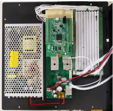
Removing the back panel reveals the control electronics.

(8)

Page 6 / 38 It is composed of three parts (in order from the picture): the power supply that converts the voltage from the grid, the electronic board that regulate the LEDs and the microcontroller board.

By further analysing the boards and reverse engineering the electronics, the following statements have been deducted:

 The LEDs intensity is changed with a programmable constant current regulation.

 The desired programmable value is sent from the microcontroller to the current regulators using a serial communication and shifting registers.

 The LEDs are powered with 15 Volts, and four are connected serially each time, forming the groups seen before.

 The maximum current transferred to the LEDs is 500mA.

4.2 F

LAWS

The objective is to use the LED Cube to generate dynamic light patterns to stimulate the eyes receptors. However, through its internal working process, it is designed to generate any desired light spectrum but not change it rapidly. Using shift registers to control the LEDs reduce greatly the frequency at which the light intensities can be changed, and it may be not suitable to use. Because all the LEDs must be changed each time a modification is done on the input, it may cause timing problems too.

The use of current regulation can influence the linearity of the LED and cause a light wavelength shift. This effect can be present with a PWM regulation too, but the impact is smaller and more linear [2]. By measuring the light peak wavelength at low and high intensity, we can see the impact of current regulation and we will be able to compare it later with the PWM regulation. Here are the peak wavelengths for a sample of the LEDs from the Cube:

Tableau 1: Peak Wavelength of the LEDs vs. LED Current %

Some of the LEDs are stable, but some are varying a lot, like the 505nm that change its wavelength of nearly 10nm. This influence can’t be neglected with the current system.

Also, the current system allows controlling the LED current with 1000 steps precision. This precision is the minimum required, having more steps is preferred.

4.3 I

NTENDED MODIFICATIONS

Change the current regulation system to a PWM regulation. This will require to change entirely the control electronics. As a software PWM is not always precise, the microprocessor will need to generate only hardware PWM. Because there are 20 different channels possible for LED outputs (counting the ones not used), the microprocessor will need 20 hardware PWM.

The power supply board will be kept, as it is satisfactory for this application. The microprocessor board will be changed entirely. The current control board will be kept too because it contains the power control for the LED supply and the power regulators for the microprocessor board.

A new software is developed to provide a better interface to the LED Cube. It will allow to control all the LEDs precisely and generate dynamic patterns to be played.

Current % 420nm 450nm 475nm 505nm 520nm 540nm 595nm 610nm 635nm 660nm

10% 418 452 476 514 529 544 593 612 634 659

50% 418 451 475 508 524 543 595 611 637 660

(9)

Page 7 / 38

5 H

ARDWARE DEVELOPMENT

5.1 M

ICROCONTROLLER 5.1.1 Choice

An already made development board will be selected as it is easier to maintain and faster to use. As the ARM family of processors is used in the precedent system, it was decided to choose one of them again.

The others necessary prerequisites are 20 hardware PWM outputs, USB communication to a PC and integrated programming IC as to not require an external tool, for ease of use. At the same time, the highest performance is desired, and the lowest cost is considered.

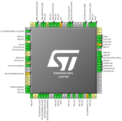
Answering all these criteria is the STM32F407VG Discovery board [3]. It contains a few pre-built features and offers a large choice of GPIO, allowing to access all 20 needed PWM for our usage. It is one of the fastest boards offered by the manufacturer STMicroelectronics.

Figure 4: STM32F4 Discovery Board

(10)

Page 8 / 38

5.2 PWM

REGULATOR 5.2.1 Description

The simplest PWM regulator is realised with the help of a transistor, driving the load in synchronisation with the PWM. But a circuit as simple as this one does not fit this application. Different specifications must be considered. The current can be high, up to 500 mA. The voltage on the regulator will vary, as all the LEDs don’t possess the same forward voltage. The timings must be precise, and the regulator must be able to operate at a frequency of at least 1000 Hz.

One of the features requested is the ability to change the current flowing through the LEDs. It must be precise and constant, as the intensity of light directly depends on it.

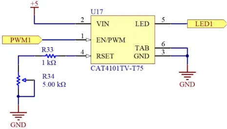
For all the reasons cited above, the choice of the regulator is directed at the CAT4101, a constant-current LED driver with PWM dimming. It is a specialised component that solves all our needs and is meant to be used in this kind of applications.

Figure 5: CAT4101, Typical application circuit (source: CAT4101 datasheet)

The current can be adjusted by changing the resistor on the RSET pin. Sadly, as it can be seen in the following figures, the relation is not linear. For our application, as the current won’t be modified very often (only during calibration), we can be satisfied with this constraint.

(11)

Page 9 / 38 As the nominal current in the LED is of 500mA, the upper limit of the current will be set to this value. Then a trimmer will be used to lower the current as desired. This will offer the possibility to change the current and protect the LEDs at the same time.

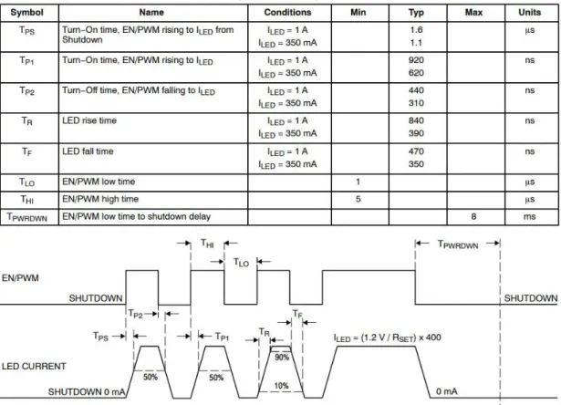
5.2.2 Timing characteristics

Another specification to take into consideration is the precision of the PWM. In fact, each time we toggle the LED output, the current and voltage will take a certain time to rise and stabilise. This characteristic is specified as follows:

Figure 7: PWM Timing (source: CAT4101 datasheet)

These characteristics don’t influence the precision with high duty cycle, because the difference will be negligible. But at lower duty values, it will have an influence. As the times are fixed, the precision will depend on the frequency used for our PWM and the duty cycle. This relation is shown in the next figure:

(12)

Page 10 / 38 Figure 8: LED Current vs. PWM Duty Cycle (source: CAT4101 datasheet)

As we will be using a PWM frequency close to 1 kHz, the small difference will occur when the duty cycle will be under 1%, getting worse as it approaches 0%. No PWM regulators can compensate entirely for this characteristic, as all components will need time to switch between the logic levels.

5.2.3 Implementation

The implementation is straightforward and follows the typical application. As mentioned, a trimmer is used to change the RSET resistor value.

Figure 9: Implementation in Circuit Maker

There are 20 different LED channels wired in the LED Cube. Only 16 of them are used for this model, but 20 channels are implemented to add LEDs as needed.

(13)

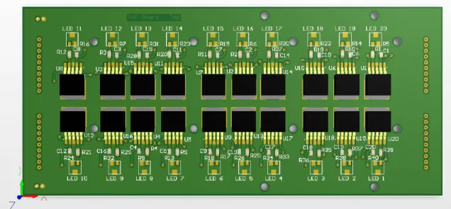
Page 11 / 38 Figure 10: 3D view of the finished board – Topside

5.2.4 Thermal specifications

The CAT4101 possess an automatic thermal shutdown protection that becomes active whenever the temperature exceeds 150°C. To prevent from reaching a temperature that high, the heatsink from the previous board will be reused.

Thermal vias have been added under the regulators and they all connect to form a thermal pad in the centre of the board. The heatsink is then fixed on top of the thermal pad and allow optimal heat transfer.

Figure 11: 3D view of the finished board - Bottom side

The power dissipation of one CAT4101 can be calculated as follows (given by the datasheet): 𝑃 = (𝑉 × 𝐼 ) + (𝑉 × 𝐼 )

With 𝑉 the voltage at the LED pin.

If we consider the worst possible case, where 𝑉 is at maximal value for the CAT4101 and 𝐼 = 500 𝑚𝐴 and we ignore 𝑉 × 𝐼 as it is inferior as 1% of the final value. We then get:

(14)

Page 12 / 38

𝑃 = 𝑉 × 𝐼 = 6 × 0.5 = 3 𝑊

Using an online tool from the company Celsia [4], we can determine the size of the required heat sink to use. By their experience, it estimates the overall heat sink volume within +/- 15% of a final design. The maximal thermal that will be dissipated is 𝑄 = 20 × 3 = 60 𝑊. The volumetric thermal

resistance 𝑅 is dependant on the air flow. As the LED Cube possess two ventilators, we will use 𝑅 = 80, as specified in the following table:

Figure 12: Airflow influence on Volumetric Thermal Resistance (source: Celsia [4])

The heatsink we are using is of dimensions 155 × 60 × 20𝑚𝑚. We can compare the desired volume with the actual volume. The desired volume is given by the equation:

𝑉 =𝑄 ∗ 𝑅 Δ𝑇

Figure 13: Comparison between estimated and actual heat sink volume (tool used: Celsia [4])

The heat sink is bigger than needed. The actual heat source power will be lower than 60 Watts in all cases, as the 𝑉 voltage is always lower than the max value of 6V in our application. Even more, in the experiences, only 4 channels are used at the same time.

(15)

Page 13 / 38

6 I

NTEGRATION INSIDE THE

LED

C

UBE

One of the objectives was to incorporate entirely the new electronics system inside the cube, with no apparent modifications from the outside.

Figure 14: New control electronics inside the LED Cube

On the left, the power supply has been kept. The new board is on the right, under the heat sink that has been reused from the central board. The microcontroller board is fixed over the central board using a standard prototype board where the cables transmitting the PWM are connected.

For programming and debugging, a different USB cable is used from the one that receives the communication data. As the programming cable won’t be needed afterwards, the USB micro cable is adapted to connect to a USB type B, identical to the original LED Cube. Using this, the external connections are similar and the whole build look the same as before.

(16)

Page 14 / 38

7 C

OMMUNICATION

P

ROTOCOL

7.1 D

ESCRIPTION

The intention of the project is to generate dynamic light patterns tailored for specific experiments that require precise timing and light intensity control.

With the current system, the PC software generates different configuration values depending on the LED calibration and desired light stimulation, that are then sent to the microcontroller. The

microcontroller will then generate the patterns intensity that will be played during the experiment based on the received configuration.

Figure 16: Current system of data transmission and output generation

As the microcontroller oversees the generation of the patterns, if the experiment is modified, the microcontroller needs to be reprogrammed at the same time to answer the needs of the new experiment. They are highly linked and dependent one from the other.

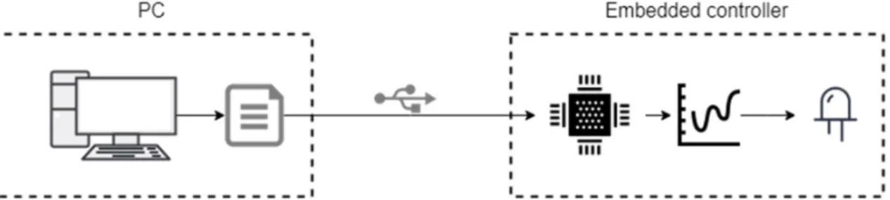
Now if we change the order in which these operations are done, and let the PC generate the patterns and send the entirety to the microcontroller, we have a more flexible system.

Figure 17: Desired system of data transmission and output generation

The microcontroller is now only responsible for one task, to play the generated patterns on the LEDs. The PC now will take care of generating these patterns and format them in a comprehensible way. It is only needed to change the code on the side of the PC when we want to change the experiment. The disadvantage is that the communication protocol is now dynamic and must adapt for any possible data, making it more difficult to implement.

(17)

Page 15 / 38

7.2 I

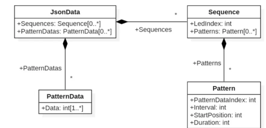
MPLEMENTATION 7.2.1 Pattern Data

The pattern data contains a set of data that is designed to be played in succession to form a pattern. As memory is limited in the microcontroller, the data is separated from the pattern itself to be reused in different cases.

7.2.2 Pattern

Using an index, the pattern is linked to a set of data. On top of that, the pattern describes how the data should be interpreted. The interval attribute indicates the time between two data point, the duration indicates for how long the pattern should be repeated until loading the next one. And finally, the start position allows beginning the pattern at a different position in the data.

Here is an example of a sinus pattern. It contains 100 data points and specifies a 10ms interval between each point. The desired duration is 3s. The sinus will then be looped 3 times to match the specifications.

Figure 18: Example of a sinus pattern 7.2.3 Sequence

A sequence contains mainly a list of patterns that will be played in order. It contains at the same time the LED index that specifies the correct LED the sequence is destined to.

7.2.4 JSON

(18)

Page 16 / 38 To store and transmit the desired data, a convention or protocol must be defined for it. As the data content can change, it must be flexible. Multiple file formats to transmit data are widely used, like XML (Extensible Markup Language [5]) and JSON (JavaScript Object Notation [6]). Both can fit our application, but JSON is easier to read, write and parse. For this reason, it was selected.

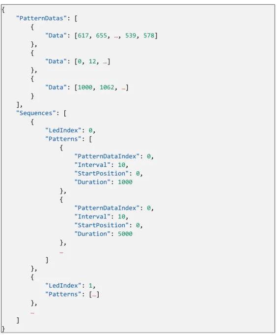
Here is an example of what the saved data looks like:

{ "PatternDatas": [ { "Data": [617, 655, …, 539, 578] }, { "Data": [0, 12, …] }, { "Data": [1000, 1062, …] } ], "Sequences": [ { "LedIndex": 0, "Patterns": [ { "PatternDataIndex": 0, "Interval": 10, "StartPosition": 0, "Duration": 1000 }, { "PatternDataIndex": 0, "Interval": 10, "StartPosition": 0, "Duration": 5000 }, … ] }, { "LedIndex": 1, "Patterns": […] }, … ] }

Figure 20: JSON data example (parts are omitted for clarity using “…”)

For ease of use, both the embedded and the computer software must be able to read this file and interpret it.

The computer software will then generate them, be able to save and open them, and finally send the content to the microcontroller to be played.

(19)

Page 17 / 38

8 E

MBEDDED SOFTWARE

8.1 STM32C

UBE

MX

AND

T

RUE

STUDIO

To facilitate the configuration of the code, a tool is provided by STMicroelectronics, named STM32CubeMX. A basic setup specifically made for the microcontroller board is available with the software.

Not only does the program generate the configuration code wanted, but it generates the project files for different kind of integrated development environment (IDE). For this project, the selected IDE is Atollic TrueSTUDIO for STM32 [7]. As Atollic is part of STMicroelectronics, TrueStudio has all the features and complete support for their boards, completely free and with no license system.

The combination of these two softwares allows an easy integration and initial configuration. Therefore all the timer’s initialisation code and the USB connection code have been generated this way.

(20)

Page 18 / 38

8.2 D

ATA

T

RANSMISSION

The data transmission is done over a USB cable. As the USB protocol is complex to implement for data transmission, we will use another functionality of the board, a virtual serial port. The hardware abstraction layer (HAL) given by STM allows to send and receive serial data without taking care of the specific USB implementation. The communication handshake is taken care of automatically, and the connected PC will see the board as a serial communication port (COM port).

Figure 22: Virtual COM port over USB The USB protocol will ensure no data is lost during the transmission.

8.3 D

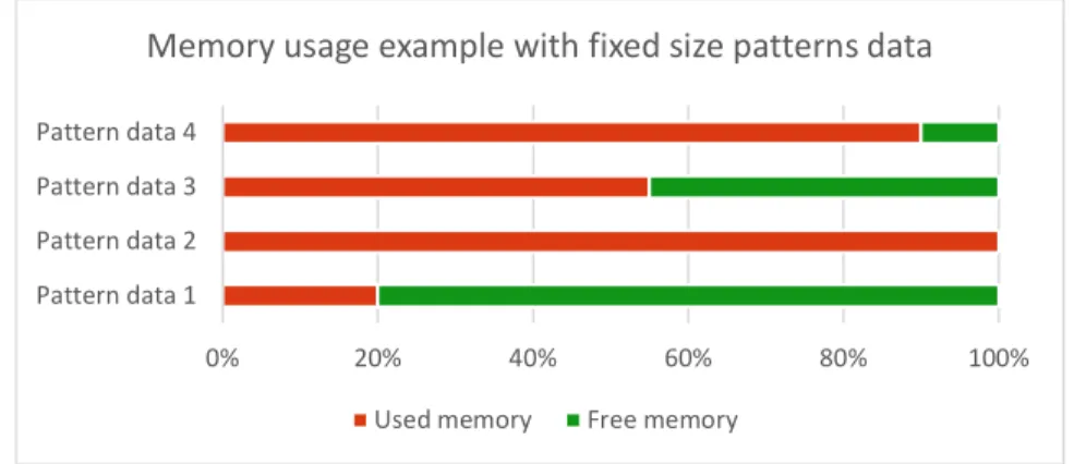
ATA REPRESENTATION

The data representation on the side of the microcontroller must be optimised to use the limited memory space to the fullest. Using dynamic memory allocation is undesired, as it risks causing memory fragmentation and maintaining the code will be more complex.

If the JSON data representation is then used, a maximum size for pattern data is defined. The data length is defined as the longest pattern desired. But then, all the shorter patterns will cause to lose data, as it can’t be used.

Figure 23: Memory usage example with fixed size patterns

The alternative is to place all the data in a contiguous array, that way no space is lost in between each pattern data. This gain comes at a small cost, we can’t modify the length of each pattern once it’s set. The whole array must be cleared, and then filled again completely.

0% 20% 40% 60% 80% 100%

Pattern data 1 Pattern data 2 Pattern data 3 Pattern data 4

Memory usage example with fixed size patterns data

(21)

Page 19 / 38 Figure 24: Memory usage example with a shared array

To realise this memory implementation, the UML representation for the JSON Data will be slightly different.

Figure 25: UML Data representation for the embedded software

The raw data seen before is still saved based on the models on the right. But now to consider the memory limitations, maximum sizes have been defined for the containers. To access and modify the data, we now must use the accessor provided. The data are referenced using their indexes in the containing class.

8.4 JSON

D

ECODING 8.4.1 Description

The JSON data files can become relatively big depending on the number and size of the patterns data. Usually, the data is decoded once the complete file has been received, this necessitates to allocate as much memory for storing the data than decoding it. We could always split the sent data to reduce this influence, but the problem will still be present at the core.

The other solution is to decode the data at the same time we receive it. Some frameworks allow to do this, but the data is usually processed only at the end when one complete element has been received. For the big arrays like the pattern data, this will not solve the problem as the received data must be

0% 10% 20% 30% 40% 50% 60% 70% 80% 90% 100%

Data array

Memory usage example example with shared array

(22)

Page 20 / 38 kept in memory. What is needed is a completely streamed JSON decoder, that decodes and store the data at the correct position in memory as soon as it has been received.

The only memory needed for this decoder is a small buffer at the start to swap with the serial port to receive and decode at the same time, some variables to hold the currently decoded value and multiple string buffers to retain the names of the variables.

The decoder will be able to find the correct destination for each data or discard it if it is not needed. 8.4.2 Implementation

The correct implementation of JSON is described on the website json.org [6]. They provide these diagrams to understand it better. We will implement a decoder working with a state machine to process the different steps. As all the functionalities of JSON are not needed, we will consider only the desired cases. If the decoder finds something it is not capable of understanding, it will just ignore it. The first step is finding the start of the file and separating data in name/value pairs. This is described as follows:

“An object is an unordered set of name/value pairs. An object begins with { (left brace) and ends with } (right brace). Each name is followed by : (colon) and the name/value pairs are separated by , (comma).” [6]

Figure 26: JSON object description (source: [6])

The string part works the same as a C string, wrapped in double quotes. The value can take different types and is more difficult to process, as each case must be taken care of. For our implementation, we will ignore the values true, false and null, as they are not needed. True and false can be replaced by an integer number. The floating points numbers are not implemented too.

Figure 27: JSON value types (source: [6])

As the values can contain objects, the JSON document can become infinitely long and complicated. This problem is usually taken care of with recursion, but because of memory and call stack limitations, it is a bad idea to use it on an embedded system.

(23)

Page 21 / 38 Multiple state machines for each “level” of the JSON document will be used instead. They will contain the previous data. Only the last level is called to process the data, and it will redirect to the next level when it finishes processing.

Arrays are a special case too because they give multiple values for a single string. As the data will be given processed one value at a time, we will need to keep a counter to index it. And because they can contain objects that can contain arrays again, the counters need to be implemented for each “level” of the decoder.

“An array is an ordered collection of values. An array begins with [ (left bracket) and ends with ] (right bracket). Values are separated by , (comma).” [6]

Figure 28: JSON array description (source: [6]) The implementation of the state machine is then as follows:

Figure 29: JSON decoder state machine

We can see the different parts described before with the colours. In blue is the array, in orange is the value and in green is an object. When a curly brace { is detected (as can be seen near the centre of the figure) a new state machine will be started and this one will be paused.

(24)

Page 22 / 38 The decoder will send all information received to a generic interface (JsonObject_t). This interface is implemented by the different levels of the JSON document (JsonMainObject, JsonPatternData, JsonSequence and JsonPattern). The decoder will use the interface to send the data to the correct recipient and use them to know if the recipient must be changed.

Figure 30: UML description of the JSON decoder and interfaces

The recipients will then change directly the program memory to store the newly received values. They will use the accessor classes described earlier (8.3 Data representation).

8.5 C

ONTROLLING THE

LED

C

UBE

The controller is very simple. It simply retrieves the serial port data and sends it to the decoder. It doesn’t do anything else except for the initialisation of the peripherals.

Then, sending commands must use the JSON protocol too. It is done by detecting string names received in the main object. For example, sending this data will start the third LED sequence:

{

"StartSequence": 3

}

Other commands to control the LED duty cycle in real time and start/stop all the sequences have also been implemented. More can be easily be added the same way. The LED cube is then controlled from the PC software.

(25)

Page 23 / 38

8.6 C

OMPLETE

UML

DIAGRAM

(26)

Page 24 / 38

9 PC

SOFTWARE

9.1 T

OOLS AND

L

IBRARIES

The previous project was using a Windows Forms Application in C++ to implement the PC program. As Microsoft dropped support for this kind of applications since Visual Studio 2012 [8], it is recommended to use C# and their new designers for a Windows Presentation Foundation (WPF) application.

C# is similar to C++, and with the .NET standard library provided by Microsoft allows to implement an application quicker and safer. As WPF was started in 2006, these kinds of applications are now well known and plenty of documentation and tutorials can be found easily.

WPF uses the architecture Model-View-ViewModel (MVVM). The view contains what is seen, as in the user interface. It is written in XAML, a declarative XML-based language made by Microsoft. When the user does an action, the view will send the information to the ViewModel, that will process it and decides of the actions. The model contains all the data the ViewModels share and need to act on. The View Model is basically a logic interface between the View and the Model.

Figure 32: Model-View-ViewModel relations The additional libraries used are:

 A user interface design library, Material Design in XAML [9] was used to give a more modern look to the application.

 A JSON decoding and encoding library, Json.Net [10].  A library to plot graphs in C#, LiveCharts [11].

 A library to do matrix mathematics, Math.Net Numerics [12]. All these libraries are free to use and open source on Github.

(27)

Page 25 / 38

9.2 F

UNCTIONALITIES

The only mandatory functionality of the program was to be able to send a configuration file and start the sequences on the LED Cube. Most of the others options the program does could just be done in code behind without visual feedback. They were done to simplify the use of the program and not need to change the code and build the application for every small modification.

9.2.1 Virtual COM port communication and configuration

The first step of the program was to connect to the LED Cube and be able to send the JSON file. In a Windows 10 computer, the correct driver is installed when the LED Cube is connected, and a COM port is automatically assigned.

The COM port number will vary on each computer, so a configuration field was added to change this parameter accordingly. The other configurations of the serial communication can also be changed. This data can then be saved to be reused the next time the software will be launched.

Then connecting to the serial port from the code is simple by using the provided class SerialPort from Microsoft libraries.

(28)

Page 26 / 38 9.2.2 Direct control of the LEDs

To test and demonstrate the LED Cube, a functionality allows to directly change the intensity of every LED channel with sliders. When the value is changed, the software will send a command to the Cube to modify the value of the duty cycle from the desired PWM channel.

Figure 34: User interface of the direct control of the LEDs duty cycle This is an example of the command used to change the PWM output:

{ "LED" : { "LedIndex" : 3, "PWM Duty" : 1000 } }

(29)

Page 27 / 38 9.2.3 JSON serialisation

No need for a custom decoder this time, as there is no memory limitation on the PC software. A few more fields have been added to the data model for better visualisation, like the names of the patterns and colour of the sequences.

Figure 36: Data model inside the PC software

Other than that, it is similar to the original model. The new fields can be sent to the LED Cube too, as they will just be ignored.

What makes this data model interesting now is that once the different classes are implemented, the process of serialisation and deserialization requires only one line of code thanks to the library Json.Net [10].

This simple process allows us to save the JSON content to a file to save the changes done and even load a configuration that was made with another program if it maintains the same model. This way, it would be possible in the future to keep this program as it is to not put too many functionalities in one place, and just use it to load the files generated elsewhere and send them to the cube. The software would be easier to maintain.

(30)

Page 28 / 38 9.2.4 Sequences visualisation

One of the first ideas for this software was the possibility to see the sequences that were about to be played on the LED Cube. The first step to achieve that goal is to represent a pattern. As we know the pattern shape, the interval and duration we can just graph it dynamically.

For this example, we will use a sinus of amplitude 1000, containing 100 data points.

Figure 37: Description of the content of a pattern visualisation

For an interval of 10ms and a length of 1.5s, the 100 data points sinus will be played 1.5 times, as we can see with the visualisation. The parameters can be changed directly in the program to observe their influence.

Now to represent a sequence, we will put multiple of these patterns on a row and add a sequence options card at the front to be able to change which LED this sequence will be played on.

(31)

Page 29 / 38 Multiple sequences are then simply put next to one another, accordingly to the JSON document.

Figure 39: User interface when visualising multiple sequences

To add or remove sequences or patterns the edit mode can be activated, and small round buttons will appear everywhere a modification can be made. This allows to quickly edit the currently loaded configuration. The edit mode can then be deactivated to make the buttons disappear.

(32)

Page 30 / 38 9.2.5 Generate preprogrammed sequences with different parameters

When testing and calibrating, the same operations are done again and again by changing only certain values. The objective here was to be able to paste directly the data from excel, and not have to rebuild the application again every time. This way, these small changes could be tested faster.

Here the example that was made is to generate specific colours based on the intensity to voltage array. This array is a result of the calibration showing the non-linearity of the LEDs. How it is generated and used will be explained by the experiences in a later section “10 Experiments and Results”.

(33)

Page 31 / 38

10 E

XPERIMENTS AND

R

ESULTS

10.1 C

ALIBRATION

The first objective was to get the intensity graphs from each LED, to observe the linearity for the main wavelength and the luminance. The old electronics in the LED Cube was using a current regulation and that was causing a noticeable shift in the LED wavelength.

If the luminance is not linear, that can be corrected by remapping the PWM values with the measurements. But nothing can be done for the wavelength. That’s why one of the main focus was on the reliability of the PWM control for this matter.

The device used to measure a given spectrum takes 3 minutes for each configuration. It was decided to do 16 different points per LED. The Cube has 16 different LED channels. The total time taken to do one set of measurements is then 12.8 hours, automated. The students from the laboratory where then of huge help in processing the data and generating the following graphs.

In this report we will focus on only one of the LED to provide context. The other measurements and graphs can be found in annexe. The chosen LED has a wavelength of 595nm, the colour is close to orange-yellow. It is the LED that was found to be the less linear and is then the best example to represent the steps involved.

10.1.1 Spectrum measurement

Each line of this graph represents a different PWM duty cycle. It was linearly increased with steps of 1/16 of the maximum value.

Figure 42: Spectrum at multiple different duty cycles of the 595nm LED -0.005 0 0.005 0.01 0.015 0.02 0.025 0.03 0.035 380 430 480 530 580 630 680 730 780 RA DI AN CE [ W / M ^2 ・ SR ] WAVELENGTH [ NM ] 595nm LED spectrum

(34)

Page 32 / 38 10.1.2 Wavelength shift

By selecting the maximum value by wavelength for each set of data we can observe any change in the colour of the LED. For comparison, here is the maximal wavelength shift for the electric current regulation, used before in the LED Cube.

We can see that it varies greatly for each LED, getting up to a 9nm difference. With the new PWM regulation, we obtain the following results:

The wavelength shift was reduced and now all types of LEDs behave similarly. The error left could be caused for two reasons:

 The PWM duty cycle induces a change in the LED wavelength. This theory was supported by the paper on LED dimming methods [2].

 4 LEDs are actually used at the same time. They will have a slightly different central wavelength due to the manufacturing process and the maximum values are actually very close.

In any cases, we can conclude that the PWM regulation is, in fact, more precise and more adapted for experiences that needs a precise light output.

Current % 420nm 450nm 475nm 505nm 520nm 540nm 595nm 635nm 660nm 10 418 452 476 514 529 544 593 634 659 50 418 451 475 508 524 543 595 637 660 100 418 450 475 505 522 543 597 639 661 Δnm 0 -2 -1 -9 -7 -1 4 5 2 PWM % 420nm 450nm 475nm 505nm 520nm 540nm 595nm 635nm 660nm 10 418 451 475 504 522 540 593 635 662 50 418 451 475 505 522 541 594 636 663 100 419 451 476 505 523 542 595 637 664 Δnm 1 0 1 1 1 2 2 2 2

(35)

Page 33 / 38 10.1.3 Luminance linearity

The luminance given by each measurement can also be compared to the duty cycle. This way, we will see the relation between the two, effectively giving the linearity. As we chose one of the worst LED to show, we can clearly see the non-linearity. The values have also been normalised with the maximum.

Figure 43: Normalised duty vs luminance (595nm LED)

It is possible to reduce the non-linearity by reducing the current in the LED. But as this will allows fewer options to use the Cube for experiments, as the maximum luminance will be reduced. The other solution that is already used in the laboratory for the previous system, is to correct the PWM duty value according to the desired luminance value. Using the graph above, we can just look at the corresponding duty cycle for every luminance value. Or even better, by characterising the curve, we can apply a mathematics identity to solve for any value.

First, we need to invert the previous graph.

Figure 44: Normalised luminance vs duty (595nm LED) y = -0.013x4_{+ 0.0267x}3_{- 0.2366x}2_{+ 1.223x} R² = 1 0 0.2 0.4 0.6 0.8 1 0 0.2 0.4 0.6 0.8 1 Lu m in an ce [% ] Duty cycle [%]

Normalised Duty vs Luminance for 595nm LED

y = 0.0616x4_{- 0.0295x}3_{+ 0.1529x}2_{+ 0.8148x} R² = 1 0 0.2 0.4 0.6 0.8 1 0 0.2 0.4 0.6 0.8 1 D ut y cy cl e [% ] Luminance [%]

(36)

Page 34 / 38 Then a polynomial trendline of order 4 is added.

𝑃𝑜𝑙𝑦𝑛𝑜𝑚𝑖𝑎𝑙 𝑡𝑟𝑒𝑛𝑑𝑙𝑖𝑛𝑒: 𝑦 = 𝑎 × 𝑥 + 𝑏 × 𝑥 + 𝑐 × 𝑥 + 𝑑 × 𝑥

Now we can convert any desired PWM value (or luminance) to have a completely linear system using the factors of the trendline.

𝐷𝑒𝑠𝑖𝑟𝑒𝑑 𝑃𝑊𝑀 𝑉𝑎𝑙𝑢𝑒: 𝑃𝑊𝑀 , 𝐿𝑖𝑛𝑒𝑎𝑟 𝑃𝑊𝑀 𝑉𝑎𝑙𝑢𝑒: 𝑃𝑊𝑀

𝑃𝑊𝑀 = 𝑃𝑊𝑀 × 𝑎 + 𝑃𝑊𝑀 × 𝑏 + 𝑃𝑊𝑀 × 𝑐 + 𝑃𝑊𝑀 × 𝑑

10.2 M

ETAMERS

“In colorimetry, metamerism is a perceived matching of the colors with different (nonmatching) spectral power distributions. Colors that match this way are called metamers.” [14]

The methodology described here along with the different calculations are the ones used for the previous system. The objective is to provide insight on one of the experiments that the LED Cube will be used for. The explanations may be incomplete as it only describes the flow process, and as the goal of the project was not to develop these experiments.

First, we will choose 4 LEDs that will cover the cones and ipRGC cells receptors. The perceived spectrum used is the following:

Figure 45: ipRGC, L-, M- and S-cone perceived spectrum (source: from the student’s calibration files) It will change slightly for everybody, but this is the one used in the laboratory.

The four LED chosen are then blue, green, red and yellow to cover the maximum spectrum. Their relative intensity is represented in the following graph.

0 0.1 0.2 0.3 0.4 0.5 0.6 0.7 0.8 0.9 1 380 430 480 530 580 630 680 N o rm al is e d L u m in an ce Wavelength [nm] L-cone*0.692839 M-cone*0.349676 S-energy ipRGC POD0.1_10degMacularP

(37)

Page 35 / 38 Figure 46: Max spectrum of the different LEDs used

A relation can be expressed between these two graphs, representing how much each LED stimulate each receptor. It is represented in our case by a matrix, called phase to cone (P2C). This matrix was determined by the students of the laboratory from the measurements made before.

We can also generate another matrix that will contain all the parameters to correct the linearity of the luminance, as explained before. It is named the intensity to voltage matrix (Int2Volt).

Then by using these two matrices, we can compute another metamer from a given colour. We can find the stimulation given to each cone by the colour using the P2C matrix:

𝐶𝑜𝑙𝑜𝑟 𝐴 = 𝑃2𝐶 ∗ 𝑆𝑡𝑖𝑚𝑢𝑙𝑎𝑡𝑖𝑜𝑛 𝑆𝑡𝑖𝑚𝑢𝑙𝑎𝑡𝑖𝑜𝑛 = L M S ipRGC = 𝑃2𝐶 ∗ 𝐶𝑜𝑙𝑜𝑟 𝐴

If we change the ipRGC part of the Stimulation vector, while maintaining the cones values, we will effectively get a metamer color.

𝐶𝑜𝑙𝑜𝑟𝐵 = 𝑃2𝐶 ∗ 𝑆𝑡𝑖𝑚𝑢𝑙𝑎𝑡𝑖𝑜n

The two colours can then be corrected with the Int2Volt matrix by using the same methodology as before.

Color = 𝐶𝑜𝑙𝑜𝑟 × 𝐼𝑛𝑡2𝑉𝑜𝑙𝑡(0) + 𝐶𝑜𝑙𝑜𝑟 × 𝐼𝑛𝑡2𝑉𝑜𝑙𝑡(1) + 𝐶𝑜𝑙𝑜𝑟 × 𝐼𝑛𝑡2𝑉𝑜𝑙𝑡(2) + 𝐶𝑜𝑙𝑜𝑟 × 𝐼𝑛𝑡2𝑉𝑜𝑙𝑡(3)

The resulting color contains the duty cycle percentage to generate it. 0 0.2 0.4 0.6 0.8 1 1.2 380 430 480 530 580 630 680 R e la ti ve l u m in an c e Wavelength [nm] Red Yellow Green Blue

(38)

Page 36 / 38

10.3 S

UMMARY OF RESULTS

Parameter Result

Duty cycle steps 65535 steps

PWM frequency 1281Hz

Wavelength shift ±2nm

Luminance linearity Corrected with polynomial trendline

The original requirement for the PWM control was of 1000 steps and a frequency of at least 1000Hz. Both of these requirements are met. For the precision, it was improved from the current regulation and the residual error is now acceptable.

The controls over the output have been improved, and the software allows fast and easy small modifications. All the experiments have not yet been reproduced or tested, but the first results with the metamer experiment are promising.

(39)

Page 37 / 38

11 C

ONCLUSION

The goal of this project was to adapt the LED Cube to be used for different experiments, like L-, M- and S-cone or ipRGC stimulations. Generating these stimuli require precise control over the LED light intensities. Even though the experiments have not been completely implemented and tested yet as they were not required for the completion of the project, the adaptation of the electronics from the current control to PWM control offer very promising results.

The wavelength shift at different light intensities has been nearly reduced completely. The residual difference is of only 1-2nm variation between minimum and maximum intensity. The luminance relation with the duty cycle has been linearized according to the same method used on the previous 4 primary display. These results are very promising to realize the experiments.

A communication protocol based on JSON has been implemented, rendering the data transmission flexible and easily alterable. The PC software and the embedded software can load the same data file to either visualise and modify it for the PC or play it in real time for the microprocessor.

The new data flow consisting in generating everything on the PC and only using the LED Cube as a part that doesn’t alter the data or is specific to an experiment will certainly facilitate modifications as the embedded software doesn’t need to be modified as frequently.

The PC software user interface has been designed to allow quick modifications to the experiments and be able to test them rapidly. With all kinds of quality of life improvements that have been added compared to the old workflow on the previous 4 primary system, it should allow using the LED Cube in a more effective way with a better visual feedback.

The development of this kind of project never stops simply because new functionalities can always be added to tailor every specific experiment possible. The code architecture has been thought to follow design patterns to be able to build easily on top of it. It is the same for the communication protocol, that can be adapted for other needs.

12 A

NNEXES

 Electronics schematics  LEDs measurements graphs

(40)

Page 38 / 38

13 R

EFERENCES AND SOURCES

[1] Wikipedia, “Intrinsically photosensitive retinal ganglion cells,” [Online]. Available: https://www.wikiwand.com/en/Intrinsically_photosensitive_retinal_ganglion_cells. [Accessed 20 August 2018].

[2] Thouslite, “LED-based Standard Lighting Environment,” [Online]. Available: http://www.thouslite.com. [Accessed 3 August 2018].

[3] N. N. A. B. a. T. K. Marc Dyble, “Impact of Dimming White LEDs: Chromaticity Shifts Due to Different Dimming Methods,” Lighting Research Center, Rensselaer Polytechnic Institute, Troy, NY, 2005.

[4] STMicroelectronics, “STM32F4Discovery,” [Online]. Available: https://www.st.com/en/evaluation-tools/stm32f4discovery.html. [Accessed 6 August 2018]. [5] Celsia, “Heat Sink Sizing Calculator,” [Online]. Available:

https://celsiainc.com/heat-sink-size-calculator/. [Accessed 7 August 2018].

[6] Wikipedia, “Extensible Markup Language,” [Online]. Available: https://www.wikiwand.com/fr/Extensible_Markup_Language. [Accessed 8 August 2018]. [7] “JSON,” [Online]. Available: https://www.json.org/. [Accessed 8 August 2018].

[8] Atollic, “TrueSTUDIO - Atollic - ST,” [Online]. Available: https://atollic.com/truestudio/. [Accessed 16 August 2018].

[9] Microsoft, “Breaking Changes in Visual C++,” 8 February 2014. [Online]. Available:

https://docs.microsoft.com/en-us/previous-versions/visualstudio/visual-studio-2012/bb531344(v=vs.110)#Anchor_1. [Accessed 20 August 2018].

[10] “Material Design In XAML,” [Online]. Available: http://materialdesigninxaml.net/. [Accessed 20 August 2018].

[11] Newtonsoft, “Json.Net - Newtonsoft,” [Online]. Available: https://www.newtonsoft.com/json. [Accessed 20 August 2018].

[12] A. Rodríguez, “Live Charts,” [Online]. Available: https://lvcharts.net/. [Accessed 20 August 2018]. [13] C. Ruegg, “Math.NET Numerics,” [Online]. Available: https://numerics.mathdotnet.com/.

[Accessed 20 August 2018].

[14] Wikipedia, “Metamerism (color),” [Online]. Available:

(41)

1 2 3 4 D D C C B B A A Title Number Revision Size A4 Date: 22.08.2018 Sheet of File: PowerCard.SchDoc Drawn By: EN/PWM 1 VIN 2 GND 3 RSET 4 LED 5 TAB 6 CAT4101TV-T75 GND R1 910 Ω R5 5.00 kΩ GND EN/PWM 1 VIN 2 GND 3 RSET 4 LED 5 TAB 6 U6 CAT4101TV-T75 +5 GND R10 910 Ω R14 5.00 kΩ GND EN/PWM 1 VIN 2 GND 3 RSET 4 LED 5 TAB 6 U10 CAT4101TV-T75 +5 GND R19 910 Ω R22 5.00 kΩ GND EN/PWM 1 VIN 2 GND 3 RSET 4 LED 5 TAB 6 U14 CAT4101TV-T75 +5 GND R27 910 Ω R30 5.00 kΩ GND EN/PWM 1 VIN 2 GND 3 RSET 4 LED 5 TAB 6 CAT4101TV-T75 GND R2 910 Ω R6 5.00 kΩ GND EN/PWM 1 VIN 2 GND 3 RSET 4 LED 5 TAB 6 U7 CAT4101TV-T75 +5 GND R11 910 Ω R15 5.00 kΩ GND EN/PWM 1 VIN 2 GND 3 RSET 4 LED 5 TAB 6 U11 CAT4101TV-T75 +5 GND R20 910 Ω R23 5.00 kΩ GND EN/PWM 1 VIN 2 GND 3 RSET 4 LED 5 TAB 6 U15 CAT4101TV-T75 +5 GND R28 910 Ω R31 5.00 kΩ GND EN/PWM 1 VIN 2 GND 3 RSET 4 LED 5 TAB 6 CAT4101TV-T75 GND R3 910 Ω R7 5.00 kΩ GND EN/PWM 1 VIN 2 GND 3 RSET 4 LED 5 TAB 6 U8 CAT4101TV-T75 +5 GND R12 910 Ω R16 5.00 kΩ GND EN/PWM 1 VIN 2 GND 3 RSET 4 LED 5 TAB 6 U12 CAT4101TV-T75 +5 GND R21 910 Ω R24 5.00 kΩ GND EN/PWM 1 VIN 2 GND 3 RSET 4 LED 5 TAB 6 U16 CAT4101TV-T75 +5 GND R29 910 Ω R32 5.00 kΩ GND EN/PWM 1 VIN 2 GND 3 RSET 4 LED 5 TAB 6 CAT4101TV-T75 GND R4 910 Ω R8 5.00 kΩ GND EN/PWM 1 VIN 2 GND 3 RSET 4 LED 5 TAB 6 U5 CAT4101TV-T75 +5 GND R9 910 Ω R13 5.00 kΩ GND EN/PWM 1 VIN 2 GND 3 RSET 4 LED 5 TAB 6 U9 CAT4101TV-T75 +5 GND R17 910 Ω R18 5.00 kΩ GND EN/PWM 1 VIN 2 GND 3 RSET 4 LED 5 TAB 6 U13 CAT4101TV-T75 +5 GND R25 910 Ω R26 5.00 kΩ GND LED1 LED2 LED3 LED4 LED8 LED7 LED6 LED5 LED9 LED10 LED11 LED12 LED16 LED15 LED14 LED13 PWM1 PWM2 PWM3 PWM4 PWM8 PWM7 PWM6 PWM5 PWM12 PWM11 PWM10 PWM9 PWM13 PWM14 PWM15 PWM16 PIR101 PIR102 COR1 PIR201 PIR202 COR2 PIR301 PIR302 COR3 PIR401 PIR402 COR4 PIR501 PIR502 PIR503 COR5 PIR601 PIR602 PIR603 COR6 PIR701 PIR702 PIR703 COR7 PIR801 PIR802 PIR803 COR8 PIR901 PIR902 COR9 PIR1001 PIR1002 COR10 PIR1101 PIR1102 COR11 PIR1201 PIR1202 COR12 _PIR1301 PIR1302 PIR1303 COR13 PIR1401 PIR1402 PIR1403 COR14 PIR1501 PIR1502 PIR1503 COR15 PIR1601 PIR1602 PIR1603 COR16 PIR1701 PIR1702 COR17 PIR1801 PIR1802 PIR1803 COR18 PIR1901 PIR1902 COR19 PIR2001 PIR2002 COR20 PIR2101 PIR2102 COR21 PIR2201 PIR2202 PIR2203 COR22 PIR2301 PIR2302 PIR2303 COR23 PIR2401 PIR2402 PIR2403 COR24 PIR2501 PIR2502 COR25 PIR2601 PIR2602 PIR2603 COR26 PIR2701 PIR2702 COR27 PIR2801 PIR2802 COR28 PIR2901 PIR2902 COR29 PIR3001 PIR3002 PIR3003 COR30 PIR3101 PIR3102 PIR3103 COR31 PIR3201 PIR3202 PIR3203 COR32 PIU101 PIU102 PIU103 PIU104 PIU105 PIU106 PIU201 PIU202 PIU203 PIU204 PIU205 PIU206 PIU301 PIU302 PIU303 PIU304 PIU305 PIU306 PIU401 PIU402 PIU403 PIU404 PIU405 PIU406 PIU501 PIU502 PIU503 PIU504 PIU505 PIU506 COU5 PIU601 PIU602 PIU603 PIU604 PIU605 PIU606 COU6 PIU701 PIU702 PIU703 PIU704 PIU705 PIU706 COU7 PIU801 PIU802 PIU803 PIU804 PIU805 PIU806 COU8 PIU901 PIU902 PIU903 PIU904 PIU905 PIU906 COU9 PIU1001 PIU1002 PIU1003 PIU1004 PIU1005 PIU1006 COU10 PIU1101 PIU1102 PIU1103 PIU1104 PIU1105 PIU1106 COU11 PIU1201 PIU1202 PIU1203 PIU1204 PIU1205 PIU1206 COU12 PIU1301 PIU1302 PIU1303 PIU1304 PIU1305 PIU1306 COU13 PIU1401 PIU1402 PIU1403 PIU1404 PIU1405 PIU1406 COU14 PIU1501 PIU1502 PIU1503 PIU1504 PIU1505 PIU1506 COU15 PIU1601 PIU1602 PIU1603 PIU1604 PIU1605 PIU1606 COU16

PIU102 PIU202 PIU302 PIU402

PIU502

PIU602 PIU702 PIU802

PIU902

PIU1002 PIU1102 PIU1202

PIU1302

PIU1402 PIU1502 PIU1602

PIR502 PIR503 PIR602 PIR603 PIR702 PIR703 PIR802 PIR803 PIR1302 PIR1303 PIR1402 PIR1403 PIR1502 PIR1503 PIR1602 PIR1603 PIR1802 PIR1803 PIR2202 PIR2203 PIR2302 PIR2303 PIR2402 PIR2403 PIR2602 PIR2603 PIR3002 PIR3003 PIR3102 PIR3103 PIR3202 PIR3203 PIU103 PIU106 PIU203 PIU206 PIU303 PIU306 PIU403 PIU406 PIU503 PIU506 PIU603 PIU606 PIU703 PIU706 PIU803 PIU806 PIU903 PIU906 PIU1003 PIU1006 PIU1103 PIU1106 PIU1203 PIU1206 PIU1303 PIU1306 PIU1403 PIU1406 PIU1503 PIU1506 PIU1603 PIU1606 PIR101 PIR501

PIR102 PIU104 PIR201

PIR601

PIR701

PIR801 PIR402 PIU404 PIR901 PIR1301 PIR902 PIU504 PIR1001 PIR1401

PIR1501

PIR1902 PIU1004 PIR2001

PIR2301

PIR2002 PIU1104 PIR2101

PIR2702 PIU1404 PIR2801

PIR3101

PIR2802 PIU1504 PIR2901

PIR3201 PIR2902 PIU1604 PIU101 POPWM1 PIU105 POLED1 PIU201 POPWM5 PIU205 POLED5 PIU301 POPWM9 PIU305 POLED9 PIU401 POPWM13 PIU405 POLED13 PIU501 POPWM14 PIU505 POLED14 PIU601 POPWM2 PIU605 POLED2 PIU701 POPWM6 PIU705 POLED6 PIU801 POPWM10 PIU805 POLED10 PIU901 POPWM15 PIU905 POLED15 PIU1001 POPWM3 PIU1005 POLED3 PIU1101 POPWM7 PIU1105 POLED7 PIU1201 POPWM11 PIU1205 POLED11 PIU1301 POPWM16 PIU1305 POLED16 PIU1401 POPWM4 PIU1405 POLED4 PIU1501 POPWM8 PIU1505 POLED8 PIU1601 POPWM12 PIU1605 POLED12 POLED1 POLED2 POLED3 POLED4 POLED5 POLED6 POLED7 POLED8 POLED9 POLED10 POLED11 POLED12 POLED13 POLED14 POLED15 POLED16 POPWM1 POPWM2 POPWM3 POPWM4 POPWM5 POPWM6 POPWM7 POPWM8 POPWM9 POPWM10 POPWM11 POPWM12 POPWM13 POPWM14 POPWM15 POPWM16

Power Card LED Cube

Corentn Barman

1.0 1

(42)

1 2 3 4 D D C C B B A A Title Number Revision Size A4 Date: 22.08.2018 Sheet of File: PowerCard_IO.SchDoc Drawn By:

PWM1 PWM2 PWM3 PWM4 PWM5 PWM6 PWM7 PWM8 PWM9 PWM10 PWM11 PWM12 PWM13 PWM14 PWM15 PWM16 PWM17 PWM18 PWM19 PWM20 LED1 LED2 LED3 LED4 LED5 LED6 LED7 LED8 LED9 LED10 LED11 LED12 LED13 LED14 LED15 LED16 LED17 LED18 LED19 LED20 EN/PWM 1 VIN 2 GND 3 RSET 4 LED 5 TAB 6 U17 CAT4101TV-T75 +5 GND R33 910 Ω R34 5.00 kΩ GND EN/PWM 1 VIN 2 GND 3 RSET 4 LED 5 TAB 6 U18 CAT4101TV-T75 +5 GND R35 910 Ω R36 5.00 kΩ GND EN/PWM 1 VIN 2 GND 3 RSET 4 LED 5 TAB 6 U19 CAT4101TV-T75 +5 GND R37 910 Ω R38 5.00 kΩ GND EN/PWM 1 VIN 2 GND 3 RSET 4 LED 5 TAB 6 U20 CAT4101TV-T75 +5 GND R39 910 Ω R40 5.00 kΩ GND PWM17 PWM18 PWM19 PWM20 LED17 LED18 LED19 LED20 1 1 2 2 J3 1 1 2 2 J5 GND GND +5 +5 C1 1uF C2 1uF C3 1uF C4 1uF C5 1uF C6 1uF C7 1uF C8 1uF C9 1uF C10 1uF C20 1uF C19 1uF C18 1uF C17 1uF C16 1uF C15 1uF C14 1uF C13 1uF C12 1uF C11 1uF GND GND +5 +5 1 2 3 4 5 6 7 8 9 10 J1 1 2 3 4 5 6 7 8 9 10 J4 1 2 3 4 5 6 7 8 9 10 J6 1 2 3 4 5 6 7 8 9 10 J2 PIC101 PIC102 COC1 PIC201 PIC202 COC2 PIC301 PIC302 COC3 PIC401 PIC402 COC4 PIC501 PIC502 COC5 PIC601 PIC602 COC6 PIC701 PIC702 COC7 PIC801 PIC802 COC8 PIC901 PIC902 COC9 PIC1001 PIC1002 COC10 PIC1101 PIC1102 COC11 PIC1201 PIC1202 COC12 PIC1301 PIC1302 COC13 PIC1401 PIC1402 COC14 PIC1501 PIC1502 COC15 PIC1601 PIC1602 COC16 PIC1701 PIC1702 COC17 PIC1801 PIC1802 COC18 PIC1901 PIC1902 COC19 PIC2001 PIC2002 COC20 PIJ101 PIJ102 PIJ103 PIJ104 PIJ105 PIJ106 PIJ107 PIJ108 PIJ109 PIJ1010 COJ1 PIJ201 PIJ202 PIJ203 PIJ204 PIJ205 PIJ206 PIJ207 PIJ208 PIJ209 PIJ2010 COJ2 PIJ301 PIJ302 COJ3 PIJ401 PIJ402 PIJ403 PIJ404 PIJ405 PIJ406 PIJ407 PIJ408 PIJ409 PIJ4010 COJ4 PIJ501 PIJ502 COJ5 PIJ601 PIJ602 PIJ603 PIJ604 PIJ605 PIJ606 PIJ607 PIJ608 PIJ609 PIJ6010 COJ6 PIR3301 PIR3302 COR33 PIR3401 PIR3402 PIR3403 COR34 PIR3501 PIR3502 COR35 PIR3601 PIR3602 PIR3603 COR36 PIR3701 PIR3702 COR37 PIR3801 PIR3802 PIR3803 COR38 PIR3901 PIR3902 COR39 PIR4001 PIR4002 PIR4003 COR40 PIU1701 PIU1702 PIU1703 PIU1704 PIU1705 PIU1706 COU17 PIU1801 PIU1802 PIU1803 PIU1804 PIU1805 PIU1806 COU18 PIU1901 PIU1902 PIU1903 PIU1904 PIU1905 PIU1906 COU19 PIU2001 PIU2002 PIU2003 PIU2004 PIU2005 PIU2006 COU20

PIC102 PIC202 PIC302 PIC402 PIC502 PIC602 PIC702 PIC802 PIC902 PIC1002

PIJ301 PIJ501 PIU1702 PIU1802 PIU1902 PIU2002

PIJ302 PIJ502 PIR3402 PIR3403 PIR3602 PIR3603 PIR3802 PIR3803 PIR4002 PIR4003 PIU1703 PIU1706 PIU1803 PIU1806 PIU1903 PIU1906 PIU2003 PIU2006 PIJ101 POLED1 PIJ102 POLED2 PIJ103 POLED3 PIJ104 POLED4 PIJ105 POLED5 PIJ106 POLED6 PIJ107 POLED7 PIJ108 POLED8 PIJ109 POLED9 PIJ1010 POLED10 PIJ201 POLED11 PIJ202 POLED12 PIJ203 POLED13 PIJ204 POLED14 PIJ205 POLED15 PIJ206 POLED16 PIJ207 PIU1705 POLED17 PIJ208 PIU1805 POLED18 PIJ209 PIU1905 POLED19 PIJ2010 PIU2005 POLED20 PIJ401 POPWM1 PIJ402 POPWM2 PIJ403 POPWM3 PIJ404 POPWM4 PIJ405 POPWM5 PIJ406 POPWM6 PIJ407 POPWM7 PIJ408 POPWM8 PIJ409 POPWM9 PIJ4010 POPWM10 PIJ601 POPWM11 PIJ602 POPWM12 PIJ603 POPWM13 PIJ604 POPWM14 PIJ605 POPWM15 PIJ606 POPWM16 PIJ607 PIU1701 POPWM17 PIJ608 PIU1801 POPWM18 PIJ609 PIU1901 POPWM19 PIJ6010 PIU2001 POPWM20 PIR3301 PIR3401 PIR3302 PIU1704 PIR3501 PIR3601 PIR3502 PIU1804 PIR3701 PIR3801 PIR3702 PIU1904 PIR3901 PIR4001 PIR3902 PIU2004 POLED1 POLED2 POLED3 POLED4 POLED5 POLED6 POLED7 POLED8 POLED9 POLED10 POLED11 POLED12 POLED13 POLED14 POLED15 POLED16 POLED17 POLED18 POLED19 POLED20 POPWM1 POPWM2 POPWM3 POPWM4 POPWM5 POPWM6 POPWM7 POPWM8 POPWM9 POPWM10 POPWM11 POPWM12 POPWM13 POPWM14 POPWM15 POPWM16 POPWM17 POPWM18 POPWM19 POPWM20

Power Card IO LED Cube

Corentin Barman

1.0 2

(43)

Page 1 of 10

LEDs Measurements

Spectrum

-0.05 0 0.05 0.1 0.15 0.2 0.25 0.3 0.35 0.4 380 430 480 530 580 630 680 730 780 Ra di an ce [ W / m ^2 ・ sr ] Wavelength [ nm ]

660nm spectrum

-0.05 0 0.05 0.1 0.15 0.2 0.25 0.3 380 430 480 530 580 630 680 730 780 Ra di an ce [ W / m ^2 ・ sr ] Wavelength [ nm ]

635nm spectrum

(44)

Page 2 of 10 -0.01 0 0.01 0.02 0.03 0.04 0.05 0.06 380 430 480 530 580 630 680 730 780 Ra di an ce [ W / m ^2 ・ sr ] Wavelength [ nm ]

595nm spectrum

-0.02 0 0.02 0.04 0.06 0.08 0.1 0.12 0.14 380 430 480 530 580 630 680 730 780 Ra di an ce [ W / m ^2 ・ sr ] Wavelength [ nm ]

540nm spectrum

(45)

Page 3 of 10 -0.05 0 0.05 0.1 0.15 0.2 0.25 380 430 480 530 580 630 680 730 780 Ra di an ce [ W / m ^2 ・ sr ] Wavelength [ nm ]

525nm spectrum

505nm spectrum

(46)

Page 4 of 10 -0.05 0 0.05 0.1 0.15 0.2 0.25 0.3 0.35 0.4 0.45 380 430 480 530 580 630 680 730 780 Ra di an ce [ W / m ^2 ・ sr ] Wavelength [ nm ]

475nm spectrum

-0.2 0 0.2 0.4 0.6 0.8 1 1.2 380 430 480 530 580 630 680 730 780 Ra di an ce [ W / m ^2 ・ sr ] Wavelength [ nm ]

450nm spectrum

(47)

Page 5 of 10 -0.1 0 0.1 0.2 0.3 0.4 0.5 0.6 0.7 0.8 380 430 480 530 580 630 680 730 780 Ra di an ce [ W / m ^2 ・ sr ] Wavelength [ nm ]

420nm spectrum

-0.02 0 0.02 0.04 0.06 0.08 0.1 0.12 0.14 0.16 0.18 380 430 480 530 580 630 680 730 780 Ra di an ce [ W / m ^2 ・ sr ] Wavelength [ nm ]

(48)

Page 6 of 10

Duty vs Luminance with linearization

White LED spectrum (550nm)

y = 0.0291x4_{- 0.0529x}3_{- 0.0264x}2_{+ 1.05x} R² = 1 0 0.2 0.4 0.6 0.8 1 1.2 0 0.2 0.4 0.6 0.8 1 1.2 Lu m ia nn ce Duty

Duty vs Luminance 660nm

(49)

Page 7 of 10 y = 0.0019x4_{- 0.012x}3_{- 0.084x}2_{+ 1.0942x} R² = 1 0 0.2 0.4 0.6 0.8 1 1.2 0 0.2 0.4 0.6 0.8 1 1.2 Lu m in an ce Duty

Duty vs Luminance 635nm

y = -0.013x4_{+ 0.0267x}3_{- 0.2366x}2_{+ 1.223x} R² = 1 0 0.2 0.4 0.6 0.8 1 1.2 0 0.2 0.4 0.6 0.8 1 1.2 Lu m in an ce Duty

Duty vs Luminance 595nm

(50)

Page 8 of 10 y = -0.0131x4_{+ 0.0367x}3_{- 0.0578x}2_{+ 1.034x} R² = 1 0.00E+00 2.00E-01 4.00E-01 6.00E-01 8.00E-01 1.00E+00 1.20E+00 0 0.2 0.4 0.6 0.8 1 1.2 Lu m in an ce Duty