Influence of the mineralogical composition on the self-potential response to advection of KCl concentration fronts through sand

HAL Id: hal-00149203

https://hal.archives-ouvertes.fr/hal-00149203

HAL is a multi-disciplinary open access archive for the deposit and dissemination of sci-entific research documents, whether they are pub-lished or not. The documents may come from teaching and research institutions in France or abroad, or from public or private research centers.

L’archive ouverte pluridisciplinaire HAL, est destinée au dépôt et à la diffusion de documents scientifiques de niveau recherche, publiés ou non, émanant des établissements d’enseignement et de recherche français ou étrangers, des laboratoires publics ou privés.

Influence of the mineralogical composition on the

self-potential response to advection of KCl concentration

fronts through sand

Alexis Maineult, Laurence Jouniaux, Yves Bernabé

To cite this version:

Alexis Maineult, Laurence Jouniaux, Yves Bernabé. Influence of the mineralogical composition on the self-potential response to advection of KCl concentration fronts through sand. Geophysical Research Letters, American Geophysical Union, 2006, 33, pp.L24311. �10.1029/2006GL028048�. �hal-00149203�

Influence of the mineralogical composition on the self-potential response to

1

advection of KCl concentration fronts through sand.

2

3

Alexis Maineult, Laurence Jouniaux and Yves Bernabé 4

5

Institut de Physique du Globe de Strasbourg, CNRS UMR 7516 – Université Louis 6

Pasteur, 5 rue Descartes, 67000 Strasbourg, France 7 8 9 ABSTRACT 10 11

We measured the self-potential (SP) response to advective transport of KCl 12

concentration fronts through two laboratory-scale sand-bodies with different 13

mineralogical composition. In pure quartz sand, the amplitude and polarity of the SP 14

signals agreed with a previously published model. In sand containing 3 % potassic 15

feldspars and 1 % micas and clays, the shape of the SP response differed significantly: the 16

amplitude was much larger than the model prediction and a change in polarity occurred 17

after the passage of the front. Furthermore, the KCl concentration in the effluent was 18

strongly reduced. We suggest that the minor mineral phases reacted with the K+ _ions,

19

trapping them during the front passage and releasing them later. Even though the 20

reactions involved are not fully identified to date, this study demonstrates that even small 21

amounts of chemically active mineral phases, such as micas or clays, can significantly 22

influence the SP signals. 23

1 INTRODUCTION

1

2

Self-potential (SP) monitoring is a geophysical method based on the measurement 3

of voltage fields naturally occurring in the Earth's subsurface. Owing to the sensitivity of 4

the self-potential to variations in groundwater flow, chemistry or temperature [e.g., 5

Corwin and Hoover, 1979], the method has been frequently used recently in subsurface

6

studies [e.g., Sandberg et al., 2002; Jardani et al., 2006]. However, the simultaneous 7

action of many different SP sources can make the interpretation difficult in terms of fluid 8

velocity and composition. To better characterize these processes, sand-box experiments 9

involving reproducible, controlled sources have been conducted in the laboratory [Ahmad, 10

1964; Maineult et al., 2004, 2005, 2006; Suski et al., 2004; Naudet and Revil, 2005]. In 11

previous works focusing on the SP response to advective transport of NaCl and FeCl2

12

concentration fronts [Maineult et al., 2004, 2005, 2006], we found that, to first order, the 13

SP signals could be modeled as the sum of: 1) an electrokinetic term, related to local 14

changes of the electrokinetic coupling coefficient with varying fluid concentration, and 2) 15

a fluid junction potential term, caused by the presence of a concentration gradient. Noting 16

that the second term should vanish when ionic species with identical mobilities are used, 17

we tried to test this prediction by running advective transport experiments using a KCl 18

solution (the mobility of K+ is equal to 96 % of the mobility of Cl–). However the 19

observations appeared to contradict this theoretical prediction. This unexpected 20

discrepancy led us to perform a new set of KCl advection experiments using a 100 % pure 21

quartz sand instead of the previously employed sand, which contained small amounts of 22

feldspars, clays and micas. The results reported here suggest that the anomalous SP 23

2 BACKGROUND

1

2

Fluid flow through a porous medium produces a downstream motion of the 3

counter-ions in excess near the charged pore-walls, resulting in a net charge separation 4

and, consequently, in the generation of the so-called electrokinetic field. Assuming no 5

surface conductivity, the electric and hydraulic potentials Ue (in V) and H (in m) are

6

related to each other by the Helmholtz-Smoluchowski equation: 7 * e g U L H ρ εζ H ησ = = ∇ ∇ ∇ (1) 8

where, ρ, ε, η and σ are the density (kg m–3), dielectric constant (F m–1), viscosity (Pa s) 9

and electrical conductivity (S m–1) of the fluid, g the gravity acceleration (m s–2) and L* 10

the electrokinetic coupling coefficient (V m–1_{). The so-called "zeta-potential" ζ (V)}

11

depends on the geochemical properties of the rock, and on the fluid composition and 12

concentration [e.g., Ogilvy et al. 1969; Ishido and Mizutani, 1981; Morgan et al., 1989; 13

Lorne et al., 1999; Guichet and Zuddas, 2003; Hase et al., 2003]. Equation (1) implies

14

that any change in the fluid concentration can modify the electrokinetic potential. 15

As ionic species diffuse along a concentration gradient, a net charge separation 16

occurs if the anion and cation mobilities are different, thus generating a counteracting 17

electrical field. The junction potential Uj (V) obeys the Planck-Henderson equation:

18

(

)

where σ– and σ+ are the anionic and cationic electrical conductivities (such as σ– + σ+ =

20

σ), ϕ the porosity, T the absolute temperature (K), R the molar gas constant (8.314 J mol– 21

1 _K–1_{), A Avogadro's number (≈6.022 10}23 _mol–1_{) and e the absolute electron charge}

(≈1.602 10–19 _{C). In the case of a symmetric, monovalent, binary salt such as NaCl or}

1

KCl, equation (2) can be simplified as: 2 * R Ae j u u C T C U C u u C α ϕ − + − + − = = + ∇ ∇ ∇ (3) 3

where α* is the junction coupling coefficient in a porous medium (V), C the salt 4

concentration (mol m–3), and u– and u+ the ionic mobilities (m2 s–1 V–1) of anions and

5

cations, respectively. 6

3 MATERIALS AND METHOD

1

2

3.1 The flow-through sand-box

3

We performed the experiments reported here in the sand-box described in detail in 4

Maineult et al. [2004, 2005] (Figure 1). Briefly, a rectangular container (44.25 × 23.75 ×

5

26.50 cm) was divided into three hydraulically connected compartments. The end-6

reservoirs (5.7- and 6.1-cm long) were used to control the flow, while the 31-cm long 7

inner one was filled up with a 21-cm height water-saturated sand-body. Precautions were 8

taken to ensure packing homogeneity and avoid air trapping. 9

A uniform, one-dimensional flow field was produced by tilting the container by an 10

angle of 4.4° (corresponding to a mean hydraulic gradient ∇H = –7.7 %) while 11

maintaining the water level in each end-reservoir constant at 20 cm from the box bottom. 12

Note that about 60 liters of primary fluid were circulated through the sand in a closed 13

circuit for several days before the experiment, to reach steady-state flow and chemical 14

equilibrium conditions. After establishing steady-state flow (i.e. stabilized flowrate, 15

conductivity and electrical potential differences), we changed the setting to open-circuit 16

and generated a sharp concentration pulse at time t = 0 by quickly adding and stirring 6 17

cm3 of saturated KCl solution in the upstream reservoir. This volume was small enough to 18

minimize the perturbation of flow (the resulting transitory, upstream water level increase 19

was only ≈0.5 mm). Generating the pulse took less than 10 s. We then stirred the 20

upstream reservoir every 2 minutes to ensure a homogeneous upstream solution. This 21

procedure produced a sharp concentration front followed by an exponentially decaying 22

tail (see Figure 2). 23

We measured the electrical potential differences (or EPDs) between a reference 1

electrode placed in the upstream reservoir and four electrodes inserted at half height in the 2

sand body, along a median, longitudinal line, at distances y equal to 5, 12, 19 and 26 cm 3

from the upstream reservoir (Figure 1). We used the small-size (i.e., 4 mm in diameter), 4

copper-copper sulfate, unpolarisable electrodes described in Maineult et al. [2004]. To 5

remove the intrinsic potential of each electrode and the constant electrokinetic signal 6

produced by the steady-state flow of the primary fluid, the EPD signals were reduced by 7

their individual initial value (all curves shown hereafter thus represent variations with 8

respect to the initial steady-state flow of the primary fluid). 9

10

3.2 Sands

11

The S4M sand from Haguenau, France, contains 96 % quartz, about 3 % potassic 12

feldspars (microcline and sanidine) and slightly more than 1 % micas and clay minerals 13

(essentially altered biotite, muscovite and illite). For the non-clay minerals, the grain 14

diameter ranges in the interval 200 – 400 µm, with a mean of 292 µm. The porosity ϕ of 15

several similarly packed sand samples was determined by dry and water-saturated 16

weighting and ranged between 36.5 and 37.0 %. By means of a column permeameter and 17

Jouniaux et al.'s [2000] electrokinetic measurement system, we measured a hydraulic

18

permeability between 20 and 22 10–12 m2. We measured the electrical conductivity of the 19

saturated sand σr for different KCl solutions with conductivity σ ranging between 2.5 and

20

100 mS m–1. The electrical formation factor F and the surface conductivity σS, defined by

21

σr = σ / F + σS, were equal to 4.70 and 0.6 mS m–1, respectively.

22

The NE34 (SIFRACO) sand from Nemours, France, is 100 % pure quartz. We did 23

not observe any traces of clays or micas. The grain diameter ranges between 75 and 320 1

µm, with a mean of 198 µm. The porosity is about 36 % and the permeability 17.5 10–12 2

m2. The formation factor was found equal to 4.90 (with σ between 50 and 500 mS m–1) 3

and there was no detectable surface conductivity, which reflects the absence of clays or 4

micas. 5

4 RESULTS

1

2

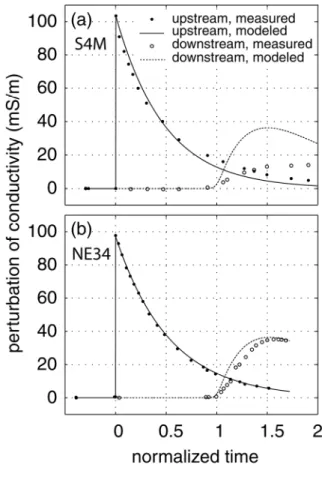
Figure 2 shows the measured fluid conductivity perturbations ∆σ(t) = σ(t) – σ0,

3

where σ0 is the conductivity of the primary fluid, for both the upstream (solid circles) and

4

downstream (open circles) reservoirs during two experiments using the S4M and NE34 5

sands. Note that to compare the results of the different experiments (the sand permeability 6

and, therefore, the flowrate varied between runs owing to slight differences in sand 7

compaction), we normalized the time by dividing it by the time needed by the front to 8

reach the downstream reservoir (neglecting the hydrodynamic dispersion) tY = vY, where

9

Y = 31 cm, and ν is the mean fluid velocity. In both experiments, the values measured in 10

the upstream reservoir are in good agreement with theoretical values (continuous lines) 11

obtained from ∆σ(t) = (σp – σ0) exp (–qt / Vup), an equation derived from mass

12

conservation [Maineult et al., 2004], where σp denotes the upstream fluid conductivity

13

just after the KCl injection, q the flowrate (m3 _s–1_{), t the elapsed time after injection (s),}

14

and Vup the water volume in the upstream reservoir (m3). In the downstream reservoir, ∆σ

15

started to increase only after the KCl front arrived at the downstream reservoir (at t = tY),

16

reached a maximum, and then slowly decreased (Figure 2). The maximum of the 17

downstream ∆σ for the S4M experiment (Figure 2a) occurs at a later normalized time and 18

is 2.5 times smaller than for NE34 (Figure 2b). The significance of this difference will be 19

discussed in section 5. 20

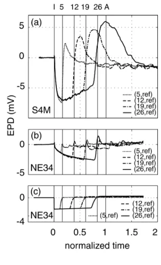
The results of one KCl front experiment in S4M sand are shown in Figure 3a. The 21

primary fluid was deionized water with a small NaCl content (σ0 = 8.5 mS m–1, σp = 112

22

mS m–1 and σp – σ0 = 103.5 mS m–1). The flow rate q was equal to 46 cm3 min–1 (v = 4.36

10–5 m s–1). Figure 3a shows the EPD curves versus normalized time (here, tY = 118.4

1

minutes). We observe a simultaneous and identical drop in all the EPDs at t = 0 to a 2

minimum value around –7 mV followed by a slow increase. Afterwards, the EPDs 3

successively jumped back to zero (and over zero) at sequential times in good agreement 4

with the theoretical arrival times of the front at the electrodes (respectively 0.16, 0.39, 5

0.61 and 0.84 in normalized time, indicated by the vertical lines in Figure 3). The jumps 6

were followed by broad and large (up to 5 mV) overshoots, whose size increased 7

significantly with distance from the upstream reservoir, and ending with a slow return to a 8

stabilized value around –1 mV. Other S4M experiments were performed using tap water 9

(σ0 ≈ 45 mS m–1, σp ≈ 145 mS m–1). The EPDs exhibited a very similar shape, although

10

the amplitude of the negative part was smaller (around –5 mV). 11

For the pure quartz sand experiment shown in Figure 3b, tap water served as 12

primary fluid, with σ0 = 46 mS m–1, σp = 143 mS m–1 and q = 34.6 cm3 min–1 (thus v =

13

3.4 10–5 m s–1, tY = 151.8 min). The initial drop of the EPDs (Figure 3b) had a magnitude

14

more than 3 times smaller than that in the S4M sand. The decrease rate was rapid at first 15

and then slowed down with time. As before, the EPDs showed a sequence of very sharp 16

increases corresponding to the theoretical arrival times of the concentration front at each 17

particular electrode, followed by a small, very narrow overshoot and, finally, a rapid 18

return to zero. Another NE34 experiment (q ≈ 42 cm3 _min–1_{, same σ}

0 and σp) gave similar

19

results. 20

5 DISCUSSION

1

2

Maineult et al. [2004] devised a conservative model (i.e., without chemical

3

reactions) to compute the downstream conductivity variation ∆σ. The results of this 4

model are represented by the dotted lines in Figure 2. Experimental data and model agree 5

quite well for the pure quartz sand only (Figure 2b). For S4M sand, the model 6

overestimates the maximum by a factor 2 and underestimates its time of occurrence. This 7

observed deficit in conductivity suggests that potassium chloride interacted with some of 8

the minor phases contained in S4M sand but not present in NE34 sand. Experiments on 9

S4M using NaCl [Maineult et al., 2005] exhibited a similar but much smaller effect (the 10

predicted maximum of ∆σ in the downstream reservoir was less 20 % higher than 11

observed); moreover, in the NaCl case, the SP signals did not exhibit positive humps as in 12

Figure 3a. Therefore, we rule out Cl– as main reacting species and conclude that the 13

chemical processes had to involve the K+ ions. 14

Maineult et al. [2004, 2005] constructed a conservative model for the SP response

15

to the advective transport of concentration fronts (note that the fluid concentration in the 16

sand-body and its evolution with time must first be determined [for details see Maineult et 17

al., 2004, 2005]). This model was validated by comparison with the results of NaCl

18

advection experiments in S4M sand. As briefly explained in section 2, the electrical 19

potential difference ∆U(ye,t) between an electrode located at ye and the reference

20

electrode is the sum of two terms: 21

(

)

(

)

(

)

(

)

U y t U y t U y t U y

∆ = ∆ + ∆⎡_⎣ − ∆ ⎤_{⎦ (4)}

22

where ∆Uj(ye,t) denotes the junction potential contribution, which is obtained by

integrating equation (2) between 0 and ye. The bracketed term corresponds to the

1

electrokinetic contribution and is obtained by integration of equation (1): 2

(

)

(

)

(

( )

( )

)

∫

(Note that the incorrectly typed equation (11) in Maineult et al. [2005] should be identical 4

to this last equation). Numerical computation of the integral in equation (5) requires 5

knowledge of the relation L*(σ(y,t)), which we experimentally estimated on S4M and 6

NE34 samples using the device and procedure described in Jouniaux et al. [2000]. For 7

each sand, we used as circulating solutions the same primary fluid as in the advection 8

experiments described above (i.e., tap water for NE34 and deionized + 30 mg L–1 NaCl 9

for S4M) to which 0, 250 or 500 mg L–1 KCl were added. Prior to the measurements, we 10

circulated these solutions in a closed-circuit for a sufficiently long time to reach chemical 11

equilibrium. In accordance with equation (1), which predicts that L* is inversely 12

proportional to σ, we determined that L* = –1.7 10–4σ–1 in the range 50 to 150 mS m–1 for 13

NE34 and L* = –2.8 10–4 σ–1 in the range 5 to 100 mS m–1 for S4M. Then, after solving 14

the conservative transport problem for KCl using the method of Maineult et al. [2004, 15

2005], we computed the EPDs from equation (4) for the NE34 sand (Figure 3c). A perfect 16

match is not obtained. The model predicts sharp, angular EPD curves at t = 0 whereas the 17

observed ones are rounded. Also, the small, narrow overshoots are not reproduced in the 18

theoretical EPDs. However, the model successfully predicts the moderate amplitude of 19

the signals, suggesting that, to first order, the EPDs are dominated by the junction 20

potential (the electrokinetics contribution, not shown here, represents less than 2 % of the 21

total potential). Note that the initial rounding of the EPDs, not predicted by our model, 22

was also observed in all our previous experiments when the reference electrode was 1

placed in the upstream reservoir, irrespective of the electrolyte used [e.g., Maineult et al., 2

2005]. The general occurrence of this effect suggests that it is more likely caused by 3

insufficient precision of the concentration modeling rather than by the SP model itself. In 4

the aforementioned previous experiments, we also always observed narrow peaks 5

accompanying the passage of the concentration front (just before or just after) but their 6

magnitude (0.3 to 0.6 mV) was much smaller than the overshoots of Figure 3a. 7

Application of our conservative SP model to S4M (using the appropriate value for L*₎

8

produces a response similar to those shown in Figure 3c and thus disagreeing completely 9

with the observations. The fact that the model is somewhat successful in the case of pure 10

quartz sand NE34 but fails totally in S4M suggests that the minor mineralogical phases 11

present in S4M (but absent in NE34) must be responsible for this effect. 12

Based on the two observations above (i.e., deficit of downstream conductivity and 13

failure of the SP model for the S4M sand) we propose that chemical reactions with the 14

minor minerals in S4M sand likely occurred, leading to trapping of K+ during the passage 15

of the concentration front and their release during passage of the tail. Prior examination of 16

the virgin S4M sand using a binocular magnifying glass showed that the mica grains were 17

essentially biotite, and, to a much smaller degree, muscovite. A new examination, carried 18

out after the NaCl transport experiments of Maineult et al.'s [2004, 2005] were performed 19

(but before the KCl ones), revealed that the biotite grains had been altered. It is well 20

known during weathering alteration, biotite is chloritized by potassium release [e.g., 21

Mitchell and Taka; 1984, and references herein] and that this reaction is quite rapid

22

[Craw, 1981; Pal, 1985; Malmström et al., 1996]. During a biotite dissolution experiment 23

the fluid remained constant at an equilibrium value (1 mmol L–1). The stability of the K+ 1

concentration was explained by a dynamic equilibration between trapping and releasing 2

of K+_{. In our experiment, the KCl concentration at the front was equal to about 7 mmol L}–

3

1_{, i.e. greater than the equilibrium concentration mentioned above. Thus, we imagine that,}

4

in experiments reported here, K+ ions were trapped by chloritized biotites as long as the 5

KCl concentration remained over this critical concentration (around 1 mmol L–1). The 6

cationic conductivity σ+ in equation (1) therefore decreases and the (negative) potential

7

gradient increases in absolute value, corresponding to the observed enhanced amplitude 8

of the initial drop (compared to the response in pure quartz sand). K+ trapping also 9

explains the deficit of conductivity in the downstream reservoir. Then, as the front 10

concentration passes below the equilibrium concentration, the trapped potassium ions 11

should be released, leading to an increase in σ+ and to the consequent change in polarity,

12

i.e., to the big positive humps observed in the SP signals. This releasing may explain the 13

fact that the maximum of the downstream conductivity was delayed in time (Figure 3a). 14

6 CONCLUSIONS

1

2

This study experimentally demonstrates that chemically active, mineral phases 3

present in rocks and soils even in small amount can strongly affect the SP response to 4

transport of ionic fronts, although we have not yet determined the precise chemical 5

mechanisms involved in the particular case studied here. The retardation effect illustrated 6

here predominantly affects the junction potential term in the SP signals. In other 7

situations, it has been shown that chemical reactions can modify the electrokinetic term as 8

well. For example, the electrokinetic coupling coefficient was significantly reduced in 9

absolute value, and even changed in sign, during calcite precipitation in sand [Guichet et 10

al., 2006]. Chemical modifications of both fluid and matrix, such as those induced by

11

dissolution/re-precipitation at high temperature, can also strongly affect the SP response 12

[Bernabé et al., 2003]. The electrokinetic behavior of rocks containing different mineral 13

phases (but without any reactions) can also be quite complicated [Hase et al., 2003]. 14

Despite their importance for field data interpretation (it seems highly probable that 15

chemically active minerals will be present in soils and rocks at any site of interest), the 16

effects of the mineralogical composition of rock and of the chemical reactions between 17

minerals and fluid on the self-potential still remain poorly documented. Many studies 18

focused on the electrokinetic potential of homogeneous media (i.e., nearly pure quartz 19

sand or pure clay powder), and few experiments have been performed to date to study the 20

junction potential in porous media. There is presently not enough information available to 21

accurately predict the SP response in strongly heterogeneous soils and rocks. The 22

incremental approach, i.e., starting from an already well-known system and modifying it 23

REFERENCES

1

Ahmad, M. U. (1964), A laboratory study of streaming potentials, Geophys. Prospect., 2

12, 49 – 64.

3

Bernabé, Y., U. Mok., A. Maineult and B. Evans (2003), Laboratory measurements of 4

electrical potential in rocks during high-temperature water flow and chemical 5

reactions, Geothermics, 32, 297 – 310. 6

Corwin, R. F., and D. B. Hoover (1979), The self-potential method in geothermal 7

exploration, Geophysics, 44, 226 – 245. 8

Craw, D. (1981), Oxidation and microprobe-induced potassium mobility in iron-bearing 9

phyllosilicates from the Otago schists, New Zealand, Lithos, 14, 49 – 57. 10

Guichet, X., and P. Zuddas (2003), Effect of secondary minerals on electrokinetic 11

phenomena during water-rock interaction, Geophys. Res. Lett., 30, 1714, doi: 12

10.1029/2003GL017480. 13

Guichet, X., L. Jouniaux, and N. Catel (2006), Modification of streaming potential by 14

precipitation of calcite in a sand-water system: laboratory measurements in the pH 15

range from 4 to 6, Geophys. J. Int., 166, 445 – 460. 16

Hase, H., T. Ishido, S. Takakura, T. Hashimoto, K. Sato, and Y. Tanaka (2003), ζ 17

potential measurements of volcanic rocks from Aso caldera, Geophys. Res. Lett., 18

30, 2210, doi: 10.1029/2003GL018694.

19

Ishido, T., and H. Mizutani (1981), Experimental and theoretical basis of electrokinetic 20

phenomena in rock-water systems and its applications to geophysics, J. Geophys. 21

Res., 86, 1763 – 1775.

22

Jardani, A., A. Revil, and J.-P. Dupont (2006), Self-potential tomography applied to the 23

determination of cavities, Geophys. Res. Lett., 33, L13401, doi: 1

10.1029/2006GL026028. 2

Jouniaux, L., M.-L. Bernard, M. Zamora, and J.-P. Pozzi (2000), Streaming potential in 3

volcanic rocks from Mount Pelée, J. Geophys. Res., 105, 8391 – 8401. 4

Lorne, B., F. Perrier, and J.-P. Avouac (1999), Streaming potential measurements 1. 5

Properties of the electrical double layer from crushed rocks, J. Geophys. Res., 104, 6

17,857 – 17,877. 7

Maineult, A., Y. Bernabé, and P. Ackerer (2004), Electrical response of flow, diffusion 8

and advection in a laboratory sand-box, Vadose Zone J., 3, 1180 – 1192. 9

Maineult, A., Y. Bernabé, and P. Ackerer (2005), Detection of advected concentration 10

and pH fronts from self-potential measurements, J. Geophys. Res., 110, B11205, 11

doi: 10.1029/2005JB003824. 12

Maineult, A., Y. Bernabé, and P. Ackerer (2006), Detection of advected, reacting redox 13

fronts from self-potential measurements, J. Contam. Hydrol., 86, 32 – 52. 14

Malmström, M., S. Banwarts, J. Lewenhagen, L. Duro, and J. Bruno (1996), The 15

dissolution of biotite and chlorite at 25°C in the near-neutral pH region, J. Contam 16

Hydrol., 21, 201 – 213.

17

Mitchell, J. G., and S. Taka (1984), Potassium and argon loss patterns in weathered 18

micas: implications for detrital mineral studies, with particular reference to the 19

triassic palaeogeography of the british isles, Sediment. Geol., 39, 27 – 52. 20

Morgan, F. D., E. R. Williams, and T. R. Madden (1989), Streaming potential properties 21

of Westerly granite with applications, J. Geophys. Res., 94, 12,449 – 12,461. 22

Naudet, V., and A. Revil (2005), A sandbox experiment to investigate bacteria-mediated 23

10.1029/2005GL022735. 1

Ogilvy, A. A., M. A. Ayed, and V. A. Bogoslovsky (1969), Geophysical studies of water 2

leakages from reservoirs, Geophys. Prospect., 17, 36 – 62. 3

Sandberg, S. K., L. D. Slater, and R. Versteeg (2002), An integrated geophysical 4

investigation of the hydrogeology of an anisotropic unconfined aquifer, J. Hydrol., 5

267, 227– 243.

6

Suski, B., E. Rizzo, and A. Revil (2004), A sandbox experiment of self-potential signals 7

associated with a pumping test, Vadose Zone J., 3, 1193 – 1199. 8

1 2

Figure 1. Experimental set-up. Flow is generated by tilting the sandbox while 3

maintaining the water levels in the upstream (u) and downstream (d) reservoirs constant. 4

The electrodes, connected to the data-logger, are represented as downward pointing 5

arrows. Their y-position (in cm) are also indicated. 6

1 2

Figure 2. Observed (dots) and predicted (lines) variations of the fluid electrical 3

conductivity in the upstream and downstream reservoirs versus normalized time for the 4

S4M (a) and NE34 (b) experiments. 5

1 2

Figure 3. Measured EPDs versus normalized time for the S4M (a) and NE34 (b) 3

experiments, and modeled EPDs for the NE34 experiment (c). The vertical lines labeled I, 4

5, 12, 19, 26 and A indicate the injection time and the computed arrival times at the sand 5

electrodes and downstream reservoir, respectively. The numbers in parentheses indicate 6

the position of the measurement electrode (the reference electrode is denoted by "ref"). 7