Atom-by-atom assembly of
defect-free one-dimensional cold atom arrays
The MIT Faculty has made this article openly available.
Please share
how this access benefits you. Your story matters.
Citation
Endres, Manuel, Hannes Bernien, Alexander Keesling, Harry Levine,
Eric R. Anschuetz, Alexandre Krajenbrink, Crystal Senko, Vladan
Vuletic, Markus Greiner, and Mikhail D. Lukin. “Atom-by-Atom
Assembly of Defect-Free One-Dimensional Cold Atom Arrays.”
Science (November 3, 2016).
As Published
http://dx.doi.org/10.1126/science.aah3752
Publisher
American Association for the Advancement of Science (AAAS)
Version
Author's final manuscript
Citable link
http://hdl.handle.net/1721.1/105257
Terms of Use
Article is made available in accordance with the publisher's
policy and may be subject to US copyright law. Please refer to the
publisher's site for terms of use.
Manuel Endres,1, 2, ∗ Hannes Bernien,1, ∗ Alexander Keesling,1, ∗ Harry Levine,1, ∗ Eric R. Anschuetz,1 Alexandre Krajenbrink,1, † Crystal Senko,1 Vladan Vuletic,3 Markus Greiner,1 and Mikhail D. Lukin1
1
Department of Physics, Harvard University, Cambridge, MA 02138, USA
2Division of Physics, Mathematics and Astronomy, California Institute of Technology, Pasadena, CA 91125, USA 3
Department of Physics and Research Laboratory of Electronics, Massachusetts Institute of Technology, Cambridge, MA 02139, USA
The realization of large-scale fully controllable quantum systems is an exciting frontier in modern physical science. We use atom-by-atom assembly to implement a novel platform for the deterministic preparation of regular arrays of individually controlled cold atoms. In our approach, a measurement and feedback procedure eliminates the entropy associated with probabilistic trap occupation and results in defect-free arrays of over 50 atoms in less than 400 ms. The technique is based on fast, real-time control of 100 optical tweezers, which we use to arrange atoms in desired geometric patterns and to maintain these configurations by replacing lost atoms with surplus atoms from a reservoir. This bottom-up approach enables controlled engineering of scalable many-body systems for quantum information processing, quantum simulations, and precision measurements.
The detection and manipulation of individual quan-tum particles, such as atoms or photons, is now routinely performed in many quantum physics experiments [1, 2]; however, retaining the same control in large-scale systems remains an outstanding challenge. For example, major efforts are currently aimed at scaling up ion-trap and superconducting platforms, where high-fidelity quantum computing operations have been demonstrated in regis-ters consisting of several qubits [3, 4]. In contrast, ul-tracold quantum gases composed of neutral atoms offer inherently large system sizes. However, arbitrary single atom control is highly demanding and its realization is further limited by the slow evaporative cooling process necessary to reach quantum degeneracy. Only in recent years has individual particle detection [5, 6] and basic single-spin control [7] been demonstrated in low entropy optical lattice systems.
This Report demonstrates a novel approach for rapidly creating scalable quantum matter with inherent sin-gle particle control via atom-by-atom assembly of large defect-free arrays of cold neutral atoms [8, 9]. We use op-tical microtraps to directly extract individual atoms from a laser-cooled cloud [10–12] and employ recently demon-strated trapping techniques [13–17] and single-atom po-sition control [18–22] to create desired atomic configura-tions. Central to our approach is the use of single-atom detection and real-time feedback [18, 21, 22] to eliminate the entropy associated with the probabilistic trap occu-pation [11] (currently limited to ninety percent even with advanced loading techniques [23–25]). Related to the fundamental concept of “Maxwell’s demon” [8, 9], this method allows us to rapidly create large defect-free atom arrays and to maintain them for long periods of time, pro-viding an excellent platform for large-scale experiments based on techniques ranging from Rydberg-mediated in-teractions [26–30] to nanophotonic platforms [31, 32] and Hubbard model physics [16, 17, 33].
The experimental protocol is illustrated in Fig. 1A. B A EM CCD vacuum cell feedback AOD Time Position
∆ν
CCDFigure 1: Protocol for creating defect-free arrays. (A) A first image identifies optical microtraps loaded with a single atom, and empty traps are turned off. The loaded traps are moved to fill in the empty sites and a second image verifies the success of the operation. (B) The trap array is produced by an acousto-optic deflector (AOD) and imaged with a 1:1 telescope onto a 0.5 NA microscope objective, which creates an array of tightly focused optical tweezers in a vacuum cham-ber. An identical microscope objective is aligned to image the same focal plane. A dichroic mirror allows us to view the trap light on a charge-coupled-device camera (CCD) while simultaneously detecting the atoms via fluorescence imaging on an electron-multiplied-CCD camera (EMCCD). The rear-rangement protocol is realized through fast feedback onto the multi-tone radio-frequency (RF) field driving the AOD.
A
C
D
10μm
B
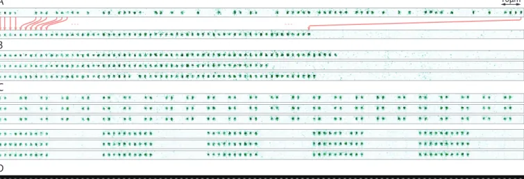
Figure 2: Assembly of regular atom arrays. (A) Single-shot, single-atom resolved fluorescence images recorded with the EMCCD before (top) and after (bottom) rearrangement. Defects are identified and the loaded traps are rearranged according to the protocol in Fig. 1, indicated by arrows for a few selected atoms. (B) Two instances of successfully rearranged arrays (first two pictures), and one instance (last picture) where a defect is visible after rearrangement. (C) The final arrangement of atoms is flexible, and we generate, e.g., clusters of two (top) or ten (bottom) atoms. Non-periodic arrangements and adjustable lattice spacings are also possible. (D) High-resolution CCD image of trap array. Our default configuration for loading atoms consists of an array of 100 tweezers with a spacing of 0.49 MHz between the RF-tones, corresponding to a real-space distance of 2.6 µm between the focused beams [34].
An array of 100 tightly focused optical tweezers is loaded from a laser-cooled cloud. The collisional blockade effect ensures that each individual tweezer is either empty or occupied by a single atom [11]. A first high-resolution image yields single-atom resolved information about the trap occupation, which we use to identify empty traps and to switch them off. The remaining occupied traps are rearranged into a regular, defect-free array and we detect the final atom configuration with a second high-resolution image.
Our implementation relies on fast, real-time control of the tweezer positions (see Fig. 1B), which we achieve by employing an acousto-optic deflector (AOD) that we drive with a multi-tone radio-frequency (RF) signal. This generates an array of deflected beams, each controlled by its own RF-tone [16, 17]. The resulting beam array is then focused into our vacuum chamber and forms an array of optical tweezers, each with a Gaussian waist of ≈ 900 nm, a wavelength of 809 nm, and a trap depth of U/kB ≈ 0.9 mK (kB, Boltzmann constant) that is homogeneous across the array within 2% [34].
The tweezer array is loaded from a laser-cooled cloud of Rubidium-87 atoms in a magneto-optical trap (MOT). After the loading procedure, we let the MOT cloud dis-perse and we detect the occupation of the tweezers with fluorescence imaging. Fast, single-shot, single-atom re-solved detection with 20 ms exposure is enabled by a sub-Doppler laser-cooling configuration that remains ac-tive during the remainder of the sequence [34] (see Figs. 2A-2C). Our fluorescence count statistics show that
in-dividual traps are either empty or occupied by a single atom [11, 34], and we find probabilistically filled arrays with an average single atom loading probability of p ≈ 0.6 (see Figs. 2A and 3A).
The central part of our scheme involves the rearrange-ment procedure for assembling defect-free arrays [34] (see Fig. 1A). In the first step, unoccupied traps are switched off by setting the corresponding RF-amplitudes to zero. In a second step, all occupied tweezers are moved to the left until they stack up with the original spacing of 2.6 µm. This movement is generated by sweeping the RF-tones to change the deflection angles of the AOD and lasts 3 ms [34]. Finally, we detect the resulting atom configuration with a second high-resolution image. These steps implement a reduction of entropy via measurement and feedback. The effect is immediately visible in the im-ages shown in Figs. 2A and 2B. While the initial filling of our array is probabilistic, the rearranged configurations show highly ordered atom arrays. Our approach also al-lows us to construct flexible atomic patterns as shown in Fig. 2C.
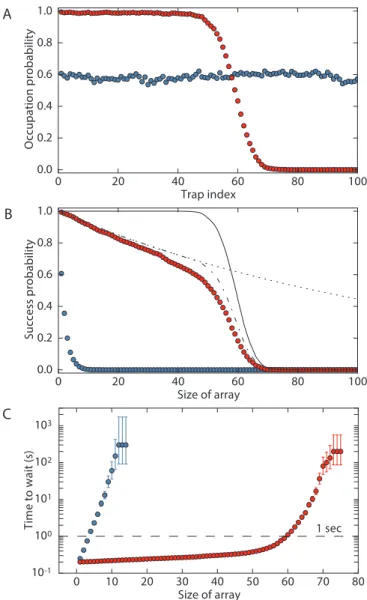
The rearrangement procedure creates defect-free ar-rays with high fidelity. This can be quantified by consider-ing the improvement of sconsider-ingle atom occupation probabil-ities (Fig. 3A) and the success probabilprobabil-ities, pN, for cre-ating defect-free arrays of length N (Fig. 3B). The single atom occupation probability in the left-most forty traps increases from ≈ 0.6 before rearrangement to 0.988(3) after rearrangement, demonstrating our ability for high-fidelity single-atom preparation. Furthermore, the
suc-0 10 20 30 40 50 60 70 80 Size of array 10-1 100 101 102 103 Ti m e to w ai t ( s) 1 sec 0 20 40 60 80 100 Size of array 0.0 0.2 0.4 0.6 0.8 1.0 Su cc ess p rob ab ili ty 0 20 40 60 80 100 Trap index 0.0 0.2 0.4 0.6 0.8 1.0 O cc up at ion p rob ab ili ty A B C
Figure 3: Quantifying the rearrangement performance. (A) The initial loading (blue circles) results in an occupa-tion probability of ≈ 0.6 for each trap in the array. After rearrangement (red circles), close to unity filling is reached on the left side of the array. (B) In the initial image, the probability of finding a defect-free length-N array (starting from the leftmost trap) falls off exponentially with N (blue circles). Following the rearrangement of all loaded traps to form the largest possible array, we demonstrate strongly en-hanced success probabilities at producing defect-free arrays (red circles). Theory curves show limits set by the total ini-tial atom number (solid line), the background limited lifetime of τ = 6.2 s (dashed line) and the product of both (dashed dotted line) [34]. (C) We show the expected amount of time to wait on average to produce a defect-free array of a given size taking into account the experimental cycle time of 200 ms (150 ms without rearrangement). Without rearrangement, the wait time grows exponentially (blue circles). Employing the rearrangement procedure, we can produce arrays of length 50 in less than 400 ms (red circles). All error bars denote 68% confidence intervals, which are smaller than the marker size in (A) and (B).
cess probabilities for creating defect-free arrays show an exponential improvement. Prior to rearrangement, the probability of finding a defect-free array of length N is ex-ponentially suppressed with pN = pN where p ≈ 0.6 (blue circles, Fig. 3B). After rearrangement, we find success probabilities as high as p30= 0.75(1) and p50 = 0.53(1) (red circles, Fig. 3B).
The same exponential improvement is observed by con-sidering the average wait time for producing defect-free arrays, given by T /pN, where T = 200 ms is the cycling time of our experiment (see Fig. 3B). For example, we are able to generate defect-free arrays of 50 atoms with an av-erage wait time of less than 400 ms (red circles, Fig. 3C). In contrast, the likelihood of finding defect-free arrays of this length without rearrangement is so small that the corresponding wait time would be on the order of several hundred years.
The success probabilities can be further enhanced through multiple repetitions of the rearrangement pro-tocol. Figure 4 illustrates the procedure in which we tar-get an atomic array of fixed length and create a reservoir from surplus atoms in a separate zone. After the initial arrangement of atoms into the target and reservoir zones, we periodically take images to identify defects in the tar-get array and pull atoms from the reservoir to fill in these defects. This enhances our initial success probabilities at producing defect-free arrays within one MOT-loading cy-cle to nearly the ideal limit (see Fig. 4C).
Finally, a similar procedure can be used for correcting errors associated with atomic loss. This becomes a signif-icant limitation for large arrays since for a given lifetime of an individual atom in the trap τ , the corresponding lifetime of the N atom array scales as τ /N . To counter this loss, we repeatedly detect the array occupation after longer time intervals and replenish lost atoms from the reservoir. As demonstrated in Fig. 4D, this procedure leads to exponentially enhanced lifetimes of our arrays.
These results demonstrate the ability to generate and control large, defect-free arrays at a fast repetition rate. The success probabilities are limited by two factors: the initial number of loaded atoms and losses during rear-rangement. For example, the average total atom number in our array is 59±5 [34], which results in the cutoff in the success probability in Fig. 3B starting from N ≈ 50 (solid line). For shorter arrays, the fidelity is mostly limited by losses during rearrangement. These losses are domi-nated by our finite vacuum-limited lifetime, which varies from τ ≈ 6 s to τ ≈ 12 s (depending on the setting of our atomic dispenser source), and are only minimally in-creased by the movement of the atoms [34]. The single atom occupation probability is correspondingly reduced by a factor exp(−tr/τ ), where tr = 50 ms is the time for the whole rearrangement procedure [34]. This results in the success probabilities of creating length-N arrays scaling as exp(−trN/τ ), which dominates the slope for N . 50 in Fig. 3B (dashed line). Currently, we reach
0 2 4 6 8 10 Hold time (s) 0.0 0.2 0.4 0.6 0.8 1.0 Su rv iv al p ro ba bil ity 1 2 3 4 5 Number of rearrangements 0.0 0.2 0.4 0.6 0.8 1.0 Su cc es s pr ob ab ili ty A B C D Time System Reservoir
∆ν
Figure 4: Creating and maintaining regular arrays using an atomic reservoir. (A) For a given target array size, surplus atoms are kept in a reservoir and used for repetitive reloading of the array. (B) These images show a 20 atom target array with a reservoir of atoms. In this set of images, defects occasionally develop in the target array and are replaced by atoms in the reservoir. The reservoir depletes as it is used to fill in defects. (C) By performing repeated rearrangements (once every 50 ms) the probability to successfully produce a defect-free array in any of these attempts increases and approaches the limit set by the number of initially loaded atoms (dashed lines). We show data for targeting 40 (purple), 50 (yellow), and 60 (green) atom arrays. Solid lines are guides to the eye. (D) Probing for defects and filling them once every 100 ms from the reservoir extends the lifetime of a defect-free array. We show data for the success probability of maintaining arrays of 20 (circles) and 40 (triangles) atoms with (red) and without (blue) replenishing atoms from the reservoir. With replenishing, the probability to maintain a defect-free array remains at a fixed plateau for as long as we have surplus atoms in the reservoir. The initial plateau value is set by the probability that no atoms in the array are lost in 100 ms (calculated value for 10 s single atom lifetime shown as the dotted line). All error bars denote 68% confidence intervals, which are smaller than the marker size in (C).
vacuum limited lifetimes only with sub-Doppler cooling applied throughout the sequence. However, the lifetime without cooling could be improved, for example, by using a different trapping laser and trapping wavelength [34].
The size of the final arrays can be considerably in-creased by implementing a number of realistic experi-mental improvements. For example, the initial loading probability could be enhanced to 0.9 [23–25] and the vacuum limited lifetime could be improved to τ ≈ 60 s in an upgraded vacuum chamber. Increasing the num-ber of traps in the current configuration is difficult due to the AOD bandwidth of ≈ 50 MHz and strong para-metric heating introduced when the frequency spacing of neighboring traps approaches ≈ 450 kHz [34]. However, implementing two-dimensional (2d) arrays could provide a path towards realizing thousands of traps, ultimately limited by the availability of laser power and the field of view of high-resolution objectives. Such 2d configura-tions could be realized by either directly using a 2d-AOD or by creating a static 2d lattice of traps (using spatial light modulators [15] or optical lattices [12]) and sort-ing atoms with an independent AOD [34]. Realistic
es-timates for the rearrangement time tr in such 2d arrays indicate that the robust creation of defect-free arrays of hundreds of atoms is feasible [34]. Finally, the repetitive interrogation techniques, in combination with periodic reservoir reloading from a cold atom source (such as a MOT), could be used to maintain arrays indefinitely.
Remarkable recent advances have been made in build-ing, explorbuild-ing, and applying engineered quantum mat-ter in systems ranging from ion traps [3] and ultracold atoms [5–7] to solid-state qubits such as superconducting qubits [4] and color-centers [35]. Atom-by-atom assembly of defect-free arrays forms a novel scalable platform with unique possibilities. It combines features that are typi-cally associated with ion trapping experiments, such as single-qubit addressability [36, 37] and fast cycling times, with the flexible optical trapping of neutral atoms in a scalable fashion. Furthermore, in contrast to solid-state platforms, such atomic arrays are formed of indistinguish-able particles and are mostly decoupled from their envi-ronment.
These features provide an excellent starting point for engineering interactions in multi-qubit experiments and
for exploring novel applications. In particular, our ap-proach can be used for the realization of logical qubits based on quantum registers consisting of up to sev-eral dozens of atomic spin qubits. The necessary entan-gling operations can be realized using atomic Rydberg states [26, 27, 29, 30]. The parallelism afforded by our flexible atom rearrangement enables efficient diagnostics of such Rydberg-mediated entanglement. For example, the use of atomic configurations demonstrated in Fig. 2C, supplemented by the repetitive reloading mechanism in Fig. 4, could allow fidelities to be optimized to their the-oretical limit [29, 30]. Similar techniques can be used for novel approaches to quantum simulations using both co-herent coupling and engineered dissipation [28, 29] and for creating large-scale maximally entangled quantum states for applications in precision measurements [38].
In addition, the realization of homogeneous arrays [34] should allow for simultaneous sideband cooling of atoms in optical tweezers [39, 40]. Ground state fractions in ex-cess of 90% have already been demonstrated, and can likely be improved via additional optical trapping along the longitudinal tweezer axes. This could enable bottom-up approaches to studying quantum many-body physics in Hubbard models [16, 17, 33], where atomic Mott in-sulators with fixed atom number and complex spin pat-terns could be directly assembled without the fluctua-tions and long cycling times associated with evaporative cooling. Moreover, these techniques could potentially be applied to create ultracold quantum matter composed of exotic atomic species or complex molecules [41, 42] that are difficult to cool evaporatively. Finally, our atom ar-rays are ideally suited for integration with hybrid atom-nanophotonic platforms [31, 32]. These can be employed to couple the atoms within a local multi-qubit register or for efficient communication between the registers using a modular quantum network architecture [3].
∗
These authors contributed equally to this work.
†
Current address: CNRS-Laboratoire de Physique Th´eorique de l’Ecole Normale Sup´erieure, 24 rue L’homond, 75231 Paris Cedex, France
[1] S. Haroche, Ann. Phys. 525, 753 (2013).
[2] D. J. Wineland, Rev. Mod. Phys. 85, 1103 (2013). [3] C. Monroe and J. Kim, Science 339, 1164 (2013). [4] M. H. Devoret and R. J. Schoelkopf, Science 339, 1169
(2013).
[5] W. S. Bakr et al., Science 329, 547 (2010). [6] J. F. Sherson et al., Nature 467, 68 (2010). [7] C. Weitenberg et al., Nature 471, 319 (2011). [8] D. S. Weiss et al., Phys. Rev. A 70, 040302 (2004). [9] J. Vala et al., Phys. Rev. A 71, 032324 (2005). [10] D. Frese et al., Phys. Rev. Lett. 85, 3777 (2000). [11] N. Schlosser, G. Reymond, I. Protsenko, and P. Grangier,
Nature 411, 1024 (2001).
[12] K. D. Nelson, X. Li, and D. S. Weiss, Nat. Phys. 3, 556
(2007).
[13] M. Schlosser, S. Tichelmann, J. Kruse, and G. Birkl, Quantum Inf. Process. 10, 907 (2011).
[14] M. J. Piotrowicz et al., Phys. Rev. A 88, 013420 (2013). [15] F. Nogrette et al., Phys. Rev. X 4, 021034 (2014). [16] A. M. Kaufman et al., Science 345, 306 (2014). [17] A. M. Kaufman et al., Nature 527, 208 (2015). [18] Y. Miroshnychenko et al., Nature 442, 151 (2006). [19] J. Beugnon et al., Nat. Phys. 3, 696 (2007).
[20] M. Schlosser et al., New J. Phys. 14, 123034 (2012). [21] W. Lee, H. Kim, and J. Ahn, Opt. Express 24, 9816
(2016).
[22] H. Kim et al., arXiv:1601.03833 (2016).
[23] T. Gr¨unzweig, A. Hilliard, M. McGovern, and M. F. An-dersen, Nat. Phys. 6, 951 (2010).
[24] B. J. Lester, N. Luick, A. M. Kaufman, C. M. Reynolds, and C. A. Regal, Phys. Rev. Lett. 115, 073003 (2015). [25] Y. H. Fung and M. F. Andersen, New J. Phys. 17, 073011
(2015).
[26] D. Jaksch et al., Phys. Rev. Lett. 85, 2208 (2000). [27] M. Saffman, T. G. Walker, and K. Mølmer, Rev. Mod.
Phys. 82, 2313 (2010).
[28] H. Weimer, M. M¨uller, I. Lesanovsky, P. Zoller, and H. P. B¨uchler, Nat. Phys. 6, 382 (2010).
[29] A. Browaeys, D. Barredo, and T. Lahaye, arXiv:1603.04603 (2016).
[30] M. Saffman, arXiv:1605.05207 (2016).
[31] J. D. Thompson et al., Science 340, 1202 (2013). [32] A. Goban et al., Nat. Commun. 5 (2014).
[33] S. Murmann et al., Phys. Rev. Lett. 115, 215301 (2015). [34] See supplementary material.
[35] D. D. Awschalom, L. C. Bassett, A. S. Dzurak, E. L. Hu, and J. R. Petta, Science 339, 1174 (2013).
[36] T. Xia et al., Phys. Rev. Lett. 114, 100503 (2015). [37] Y. Wang, X. Zhang, T. A. Corcovilos, A. Kumar, and
D. S. Weiss, Phys. Rev. Lett. 115, 043003 (2015). [38] P. K´om´ar et al., arXiv:1603.06258 (2016).
[39] A. M. Kaufman, B. J. Lester, and C. A. Regal, Phys. Rev. X 2, 041014 (2012).
[40] J. D. Thompson, T. G. Tiecke, A. S. Zibrov, V. Vuleti´c, and M. D. Lukin, Phys. Rev. Lett. 110, 133001 (2013). [41] J. F. Barry, D. J. McCarron, E. B. Norrgard, M. H.
Stei-necker, and D. DeMille, Nature 512, 286 (2014).
[42] N. R. Hutzler, L. R. Liu, Y. Yu, and K.-K. Ni, arXiv:1605.09422 (2016).
———————– Acknowledgments
We thank K.-K. Ni, N. Hutzler, A. Mazurenko and A. Kaufman for insightful discussion. This work was sup-ported by NSF, CUA, NSSEFF and Harvard Quantum Optics Center. HB acknowledges support by a Rubicon Grant of the Netherlands Organization for Scientific Research (NWO).
———————–
Supplementary Materials Materials and Methods Figs. S1 to S5
SUPPLEMENTARY MATERIAL Contents 1 Experimental Sequence 6 1.1 Trap loading 6 1.2 Imaging 7 1.3 Feedback 7 2 Experimental Methods 7 2.1 Generating 100 traps 7 2.2 Effects of intermodulation 8
2.3 Optimizing trap homogeneity 8
2.4 Characterizing trap homogeneity 8
2.5 Moving traps 8
2.6 Lifetimes 9
3 Prospects for extensions to 2D arrays 10
3.1 Method 1: Row or column deletion and
rearrangement 10
3.2 Method 2: Row-by-row rearrangement 10 3.3 Expected performance and scalability 11 4. Movies of the rearrangement procedures 11
1 EXPERIMENTAL SEQUENCE 1.1 Trap loading
We use an external-cavity diode laser at ≈ 809 nm to seed a tapered amplifier (Moglabs, MOA002), which pro-vides 1.8 W of output power. The resulting beam is cou-pled into a single-mode fiber, and passed through three laser clean-up filters (Semrock LL01-808). This results in a 4 mm beam with ≈ 550 mW of power, which is split into an array of beams by an acousto-optic deflector (AOD) (AA Opto-Electronic model DTSX-400-800.850). These beams pass through a 1:1 telescope with 300 mm focal length and are then focused by a 0.5 NA microscope objective (Mitutoyo G Plan Apo 50X) into our vacuum chamber to form an array of optical tweezers (Fig. 1B of the main text). These tweezers have a waist of ≈ 900 nm, and their centers are separated by 2.6 µm. Each beam has ≈ 1 mW of optical power, corresponding to a trap depth of ≈ 0.9 mK for87Rb atoms.
The experimental sequence begins by laser cooling thermal 87Rb atoms in a magneto-optical trap (MOT) around the traps for 100 ms (Fig. S1A). We use a gradi-ent field of 9.7 G/cm, and three intersecting retroreflected beams that are 17 MHz red detuned of the free space F = 2 → F0 = 3 transition, overlapped with repumper beams resonant with the free space F = 1 → F0= 2 tran-sition. One of these beams is perpendicular to the optical table, and the other two are parallel to it (intersecting at
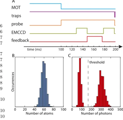
0 20 40 60 80 100 Number of atoms O cc ur re nc es 0 100 200 300 400 500 Number of photons threshold MOT traps probe EMCCD feedback time (ms) 100 120 140 160 180 200 A B C
Figure S1: Experimental sequence and atomic signal. A) Pulse diagram of the experimental sequence. B) Distri-bution of number of initially loaded atoms. C) Sample fluo-rescence count distribution for a single trap during 20 ms of exposure.
an angle of ≈ 120◦ due to the geometric restriction im-posed by the high resolution objectives). All three beams have a diameter of ≈ 1.5 cm, and carry ≈ 1.5 mW of cooling light and ≈ 0.4 mW of repumping light each. To reduce the necessary time to load the MOT, we shine UV light from a diode at 365 nm directly on the region of the glass cell within which the MOT is loaded [S1].
After 100 ms, the magnetic field gradient and the MOT beams are turned off to allow the MOT to dissipate over 28 ms. At the same time we turn on a set of probe beams which are 20 MHz red-detuned from the bare atom F = 2 → F0 = 3 transition. The probe beams have the same geometric configuration as the MOT beams, but they have ≈ 50 times less power, and a diameter of ≈ 1 mm, which largely reduces background light due to stray reflections during imaging. The probe beams fur-ther cool the atoms through polarization-gradient cool-ing, and are left on for the remainder of the sequence.
The result of this process is the probabilistic load-ing of atoms into the traps. For the data presented in Fig. 3 of the main text we loaded on average 59±5 atoms (Fig. S1B).
1.2 Imaging
The EMCCD camera (Andor iXON3) is triggered 128 ms after the beginning of the experimental sequence and acquires an image over the following 20 ms. Cooling light from the probe beams is scattered by the atoms and collected on the EMCCD, forming an image of the atoms in the array. Based on the collected photon statistics for each trap, we can set clear thresholds to determine the presence of an atom in a trap (see Fig. S1C). Further-more, the bimodal nature of the photon statistics is an indication that the traps are occupied by either 0 or 1 atom.
1.3 Feedback
Once the EMCCD has finished acquiring the signal, the image file is transferred over the following 10 ms to a computer which determines trap occupations, using pre-calibrated regions of interest and threshold counts for each trap, in sub-ms time. Using this information, the computer finds the correct pre-calculated waveform to displace each occupied trap during 3 ms from its initial position to its final position, and then adds up all of them into a multi-tone frequency-sweep waveform. This com-putation takes ≈ 0.2 ms for each trap to be displaced. Once the waveform is ready, it is sent to the AOD to perform the trap displacement, and then it goes back to producing the original set of 100 traps. It is important to note that the rearrangement waveform is only calculated for loaded traps, which means that all empty traps are turned off for the duration of the rearrangement but are restored immediately afterwards, so that the trap array returns after rearrangement to its original configuration. After rearrangement, there is a ≈ 7 ms buffer time before taking another 20 ms exposure image with the EMCCD. The entire process, consisting of image acquisition, trans-fer, analysis, waveform generation, rearrangement, and buffer, takes a total of 50 ms.
Currently, the profile of the frequency sweeps is cal-culated to be piece-wise quadratic in time, over a du-ration of 3 ms. For shorter transport times we observe an increase in the number of atoms lost during rear-rangement. For the experiments reported in the main text, atom losses are only slightly increased compared to the expected lifetime in static traps (see Fig. S2). These losses depend on the distance that the atoms move, and it is possible that they could be reduced by changing the length or the profile of the frequency sweep to minimize acceleration and jerk during the trajectory. However, the fidelity of our rearrangement would not be significantly improved by minimizing these losses (see Fig. 3B of the main text).
0 10 20 30 40 50 60
Distance traveled (# lattice spacings) 0.00 0.05 0.10 0.15 0.20 0.25 Loss probability
Figure S2: Rearrangement losses. Losses as a function of total distance traveled by the atom during rearrangement for the dataset presented in Fig. 3 of the main text. The dashed line represents the expected loss for a stationary trap with 6.2 s lifetime.
2 EXPERIMENTAL METHODS
2.1 Generating 100 traps
When driving the AOD with a single radio frequency (RF) tone, a portion of the input beam is deflected by an angle θ that depends on the frequency ω of the tone. By applying 100 different RF tones {ω1, . . . , ω100}, we generate 100 beams with output angles {θ1, . . . , θ100}, where θi = θ(ωi). The waveform that we send into the AOD is initially calculated by a computer that samples the desired waveform in the time-domain with a pling rate of 100 MHz. We stream these waveform sam-ples to a Software Defined Radio (SDR) (Ettus Research, model USRP X310, daughterboard UBX 160) which per-forms digital-analog conversion, low-pass filtering, and subsequent analog IQ upconversion by a frequency of ωup= 74 MHz, and outputs an analog waveform, which we then amplify and send to the AOD. The waveform that we calculate initially is given by:
100 X
i=1
Aieiφiei(ωi−ωup)t,
with Ai and φi being the real amplitude and phase, re-spectively, of the RF tone with frequency ωi. Since we generate all tones in the same waveform (relative to the same local oscillator inside the SDR), the tones in our waveform have well-defined phases {φi} relative to one another. Also, since all the frequencies we use are integer multiples of 1 kHz, we calculate a 1 ms waveform which is streamed on a loop without needing to continuously generate new samples.
2.2 Effects of intermodulation
The finite power bandwidth, along with other imper-fections of our system (RF amplifier and AOD) generate a nonlinear response to the input signal. To the lowest or-der nonlinearity, the system acts as a mixer and generates new tones at the sum and difference of the input frequen-cies. For example, for two tones, A1eiφ1eiω1t, A2eiφ2eiω2t, at the input, there will be a corresponding set of tones at the output:
E1,2− = A−1,2ei(φ1−φ2)ei(ω1−ω2)t,
E+1,2= A+1,2ei(φ1+φ2)ei(ω1+ω2)t
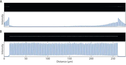
These terms are far removed from the main set of de-sired tones {ωi} and can in principle be filtered by fre-quency. However, they seed the next order of nonlinearity. The next order of nonlinearity contains the mixing of these first order nonlinearities with the original tones. For example, with two tones we would now see a mixing of the (ω1− ω2) tone with the original ω1 tone to produce a sum tone at (2ω1− ω2) and a difference tone at ω2. Similarly, the (ω1− ω2) tone would mix with the original ω2 tone to produce a tone at (2ω2− ω1) and ω1. If the phases of each input tone {φi} are not carefully selected, these intermodulations interfere destructively with the original tones, as shown in Fig. S3A.
2.3 Optimizing trap homogeneity
We address the issue of intermodulations by adjusting the phases of the different RF tones to almost completely cancel out the nonlinearities. As a first step, we generate a computer simulation of 100 tones evenly spaced in fre-quency and with random phases, and equal amplitudes. For each pair of traps {i, j}, we calculate the difference tone Ei,j−. By starting with random initial phases, the difference tones nearly completely destructively interfere with one another. We then optimize each phase, one at a time, to further reduce the sum of all difference tones P E−
i,j. After this, we proceed to generate the waveform to be streamed onto the SDR. The starting amplitudes for each tone are selected such that they individually pro-duce a single deflection carrying the correct amount of optical power. The frequencies span from 74.5 MHz to 123.01 MHz in steps of 0.49 MHz.
The next step in optimization consists of imaging the focused trap array on a CCD and performing 2D Gaus-sian fits. We use the amplitude of these fits to feed back on the amplitude of the individual tones. Once all the fit-ted amplitudes are approximately uniform, we continue to the last step of optimization.
Since we are interested in the uniformity of the traps at the positions of the atoms, we measure the AC Stark
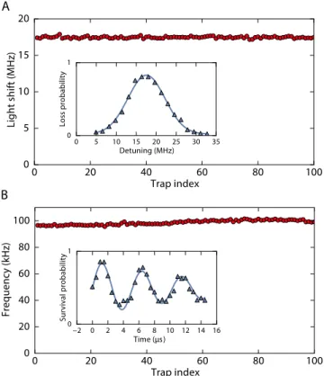
shifts induced by the traps, and use these values to feed back on the amplitude of each tone. In order to extract the AC Stark shift, we shine a single laser beam onto the trapped atoms for 10 µ s, and measure the loss prob-ability introduced by this “pushout” beam as a function of detuning from the bare F = 2 → F0 = 3 resonance (Fig. S4A inset). From the fits we extract the individual lightshift for each trap and use these values to perform feedback on the amplitudes. We repeat the procedure un-til the shifted resonances are uniform to within ≈ 2% across the trap array (Fig. S4A). At this point we have a set of optimal amplitudes {Aopti } and phases {φopti } as-sociated with the RF frequencies {ωi} (Fig. S3B). We interpolate between the values of {Aopti } to define the optimal amplitude as a function of frequency Aopt(ω).
2.4 Characterizing trap homogeneity
To characterize the homogeneity of the final trap con-figuration, we perform experiments to determine the AC Stark shift and trap frequency for each trap in the array (Fig. S4).
As outlined in the previous section, the measurement of the AC Stark shift is used to equalize the traps. We find an average shift of 17.5 MHz with a standard deviation of 0.1 MHz across the whole array.
The trap frequency (Fig. S4B) is found through a re-lease and recapture technique [S2]. We obtain the radial frequency from a fit to the probability of retaining an atom as a function of hold time (Fig. S4B inset). We find the average trap frequency to be 98.7 kHz with a stan-dard deviation of 1.7 kHz across the array. Combining these measurements with an independent determination of the waist, we estimate a trap depth of ≈ 0.9 mK.
2.5 Moving traps
For most of the experimental sequence time, the traps are static. However, during short bursts we stream new waveforms to the AOD to rearrange them, and the atoms they hold. We move our traps by sweeping the frequencies {ωi(t)} of the tones that correspond to the traps we wish to move, in a piecewise-quadratic fashion. This way, the atoms experience a constant acceleration a for the first half of the trajectory, and −a for the second half. Dur-ing the sweep, we also continuously adjust the amplitude of the RF tone to match the optimized amplitude for its current frequency: Ai(t) = Aopt(ωi(t)). Further, by slightly adjusting the duration of each sweep, we enforce each trap to end with the optimal phase corresponding to its new position.
Using these parameters we pre-calculate all waveforms to sweep the frequency of a tone at any given starting
In te ns ity 0 50 100 150 200 250 Distance (μm) In te ns ity A B
Figure S3: Generating uniform traps. Nonlinearities inside the AOD and RF amplifier cause frequency mixing. (A) Setting identical phases for each input tone results in intermodulations that strongly interfere with the intended frequency tones and significantly distort the trap amplitudes. (B) By optimizing the phases {φi} and amplitudes {Ai} of the RF tones we can
reduce intermodulations and generate homogeneous traps.
frequency in our array to any given final frequency, over 3 ms. This amounts to 1002 precalculated trajectories.
2.6 Lifetimes
The lifetime for each trap is found by an exponential fit to the probability of retaining an atom as a function of time. Under optimal conditions, this results in an av-erage lifetime for the traps in our array of 11.6 s with a standard deviation of 0.5 s across the array. However, this value depends on the background pressure inside the vacuum chamber and therefore depends on the current with which we drive our dispenser atom source. For the measurements presented in Fig. 3 of the main text, an average lifetime of 6.2 s was found from independent cal-ibration measurements.
In these measurements, we apply continuous laser cool-ing throughout the hold time. We observe that without continuous cooling, the lifetime is reduced compared to these values. The retention as a function of time in this case does not follow a simple exponential decay (indica-tive of a heating process), and we define the time at which the retention probability crosses 1/e to be the lifetime. For the standard configuration in the main text (100 traps with 0.49 MHz spacing between neighboring fre-quencies), we find a lifetime of ≈ 0.4 s. While we have not characterized the source of the lifetime reduction in detail, we have carried out a number of measurements in different configurations to distinguish various effects:
• Generating a single trap by driving the AOD with a single frequency from a high-quality signal gen-erator (Rhode & Schwartz SMC100A), we find a
lifetime of ≈ 2 s. This indicates that there are ad-ditional heating effects, such as photon scattering from trap light or intensity noise, that are indepen-dent of the use of the SDR or the fact that we drive the AOD with a large number of frequencies. Pos-sible improvements include using further detuned trap light and improving our intensity stabilization. Furthermore, in a separate experiment [S3], we ob-served that using a Titanium-Sapphire laser instead of a TA significantly improved trap lifetimes even at the same trapping wavelength.
• Generating a single trap by driving the AOD with a single frequency from the SDR, we find a lifetime of ≈ 1 s. This indicates that the RF-waveforms from the SDR could have additional phase or intensity noise. A possible source is the local oscillator used for IQ upconversion in the SDR, which could be replaced with a more phase-stable version.
• We observe the same trap lifetime of ≈ 1 s when driving the AOD with 70 frequencies at a spacing of 0.7 MHz using the SDR. This indicates that, in principle, there is no lifetime reduction associated with driving the AOD with a large number of fre-quencies.
• We observe a reduction of lifetime for frequency spacings smaller than ≈ 0.65 MHz. For example, we found a lifetime of ≈ 0.4 s, when setting the fre-quency spacing to 0.49 MHz. (This lifetime is un-changed by increasing the number of traps from 70 to 100.) We interpret this effect to be the re-sult of interference between neighboring traps. Due to the finite spatial overlap of the tweezer light,
0 20 40 60 80 100 Trap index 0 5 10 15 20 Li gh t s hi ft (M H z) 0 5 10 15 20 25 30 35 Detuning (MHz) 0 1 Lo ss pr ob abi lit y 0 20 40 60 80 100 Trap index 0 20 40 60 80 100 Fr eq ue nc y (k H z) −2 0 2 4 6 8 10 12 14 16 Time (μs ) 0 1 Su rviv al proba bi lit y A B
Figure S4: Characterization of trap and atom proper-ties. (A) The trapping light causes a lightshift on the atomic resonances that depends on the amplitude of the trap. The measured lightshifts across the array are used to optimize the RF amplitudes {Ai}. This process results in homogeneous
traps with lightshifts that are uniform to within ≈ 2%. Inset shows the result of a pushout measurement (see text) on trap 26 that is used to determine the individual lightshift. (B) The trap frequencies are determined from a release and recapture measurement [S2] (see inset for trap 26). The errors from the fits are smaller than the marker size for all the figures.
a time-dependent modulation occurs with a fre-quency given by the frefre-quency spacing between neighboring traps. When bringing traps closer to-gether, both the spatial overlap increases and the modulation frequency approaches the parametric heating resonance at ≈ 200kHz given by twice the radial trapping frequency.
We would like to stress that these effects only play a role after the rearrangement procedure is completed. During rearrangement, continuous laser cooling is a valid and powerful method to reduce heating effects. Additionally, the flexibility of our system makes it possible to load and continuously cool atoms in a set of closely spaced traps, and to rearrange the filled traps to an array with larger separations, at which point cooling can be turned off. This method of rearrangement takes advantage of the large number of atoms that can be initially loaded in our set of 100 traps separated by 0.49 MHz, while elim-inating the effect of interference by setting a larger final
frequency separation of, for example, 0.7 MHz. Further-more, atoms could also be transferred into a fully “static” trap array, such as an optical lattice, after rearrangement. However, even with optimal cooling parameters, heat-ing effects cannot be always compensated. For example, we observed a significant reduction of lifetime for fre-quency spacings below ≈ 0.45 MHz even with continuous laser cooling. This sets a limit on the maximum number of traps that can be generated within the bandwitdh of our AOD, and therefore limits the final sizes of the atomic arrays.
3 PROSPECTS FOR EXTENSIONS TO 2D ARRAYS
In this section we will discuss possible extensions of our method to form uniformly filled two-dimensional (2d) ar-rays. We will describe two different rearrangement strate-gies and compare their performance given realistic pa-rameters for loading efficiencies and lifetimes.
3.1 Method 1: Row or column deletion and rearrangement
Using a 2d AOD we could generate a 2d array of optical tweezers using two sets of RF tones, one set correspond-ing to rows and the other correspondcorrespond-ing to columns. After loading atoms probabilistically into the array, it would be possible to eliminate each defect by turning off the RF frequency that generates either the row or the column containing the defect, and then transport all remaining rows and columns to form a defect-free uniform array.
3.2 Method 2: Row-by-row rearrangement
A different approach is to generate a static two-dimensional array of traps using techniques such as op-tical lattices or spatial-light modulators. In a first step, atoms would be probabilistically loaded into this static array. After loading, we could use an independent AOD to generate a linear array of traps, deeper than the ones forming the static array and overlapping precisely with one row of static traps. By rearranging the linear array, we could transfer the atoms to their final locations in the static configuration, where they would remain after turn-ing off the traps used for transport. Doturn-ing this for each row would make it possible to fill an entire region of the static 2d array.
A B
C D
Initial # of columns Initial # of columns
Initial # of r ow s Initial # of r ow s M ethod 1 M ethod 2 0 200 400 600 800 100 300 500 700 Final # of A toms 10 20 30 40 50 10 20 30 40 50 10 20 30 40 50 10 20 30 40 50 20 30 40 50 20 30 40 50 40 80 120 160
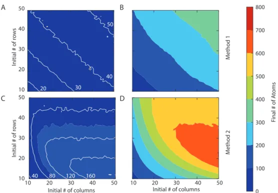
Figure S5: Projections for 2D system sizes. Expected number of atoms in defect free rectangular arrays generated through the “Row or column deletion and rearrangement method” with 0.6 loading efficiency and 10 s lifetime (A), and with 0.9 loading efficiency and 60 s lifetime (B). Expected number of atoms in defect free rectangular arrays generated through the “Row-by-row rearrangement method” with 0.6 loading efficiency and 10 s lifetime (C), and with 0.9 loading efficiency and 60 s lifetime (D).
3.3 Expected performance and scalability
The final size of the array will depend on the initial loading efficiency, while the probability to have a defect-free array after rearrangement will depend on the atom lifetimes in the traps, and the total feedback time. This time consists of several blocks: image taking, image trans-fer, waveform calculation, and trap movement. We can take an image in 20 ms. The time it takes to transfer the image from the camera to the computer takes a minimum of 9 ms and each row of atoms adds 0.8 ms to the transfer time. Analyzing the image to determine the location of the atoms and necessary frequency sweeps can be done in sub-ms time. Generating the waveform takes ≈ 0.2 ms for each sweep necessary. This time scales as the final number of atoms (O(N )) for method 2, and with the fi-nal number of rows and columns (O(N1/2)) for method 1. Finally, the rearrangement itself takes 3 ms for each set of frequency sweeps: for method 1 there are two sweeps, and for method 2 the number of sweeps equals the number of rows.
Figure S5 shows the result of a Monte Carlo simula-tion for the expected number of atoms in a defect-free rectangular array using two sets of parameters, and both rearrangement methods described above. Given our cur-rent loading efficiency of 0.6 and vacuum-limited lifetime of ≈ 10 s, we can expect more than 160 atoms in the final defect-free configuration (Fig. S5A, C). However, if
we were to upgrade our vacuum setup to increase the lifetime from 10 s to 60 s, and we increased the load-ing efficiency to 0.9 usload-ing currently available techniques [S4, S5, S6], we could expect more than 600 atoms in defect-free configurations (Fig. S5B, D). These numbers were calculated by simulating a sequence that performed repeated rearrangement until no more defects appeared, and every point on the plot is the average of 500 simula-tions.
4. MOVIES OF THE REARRANGEMENT PROCEDURES
(See ancillary files)
VS1: Rearrangement procedure. This video shows con-secutive pairs of atom fluorescence images. Each pair consists of an initial image showing the random load-ing into the array of traps and a subsequent image after the loaded atoms have been rearranged to form a regular array. The sequence of images demonstrates the effective-ness of the procedure to reduce the entropy associated with the random initial positions of the atoms by order-ing them in long, uninterrupted chains. The 1 Hz cycle rate in the video is slowed down by a factor of five relative to the 5 Hz experimental repetition rate.
VS2: Lifetime extension of 20 atom array. This video shows consecutive fluorescence images of atoms being
re-arranged from an initial probabilistic loading into an or-dered array of 20 atoms and a reservoir formed by surplus atoms. The length of the target array is kept constant by transporting atoms from the reservoir to replace lost atoms in the target array. This technique makes it possi-ble to extend the average lifetime of a defect-free 20 atom array to ≈ 8 s, at which point the reservoir typically has depleted. The 10 Hz frame rate of this video accurately reflects the rate at which these images were acquired.
VS3: Lifetime extension of 40 atom array. This video shows consecutive fluorescence images of atoms being re-arranged from an initial probabilistic loading into an or-dered array of 40 atoms and a reservoir formed by surplus atoms. The length of the target array is kept constant by transporting atoms from the reservoir to replace lost atoms in the target array. This technique makes it possi-ble to extend the average lifetime of a defect-free 40 atom array to ≈ 2 s, at which point the reservoir typically has depleted. The 10 Hz frame rate of this video accurately reflects the rate at which these images were acquired.
∗
These authors contributed equally to this work.
†
Current address: CNRS-Laboratoire de Physique Th´eorique de l’Ecole Normale Sup´erieure, 24 rue L’homond, 75231 Paris Cedex, France
[S1] C. Klempt et al., Phys. Rev. A 73, 013410 (2006). [S2] Y. R. P. Sortais et al., Phys. Rev. A 75, 013406 (2007). [S3] J. D. Thompson et al., Science 340, 1202 (2013). [S4] T. Gr¨unzweig, A. Hilliard, M. McGovern, and M. F.
An-dersen, Nat. Phys. 6, 951 (2010).
[S5] B. J. Lester, N. Luick, A. M. Kaufman, C. M. Reynolds, and C. A. Regal, Phys. Rev. Lett. 115, 073003 (2015). [S6] Y. H. Fung and M. F. Andersen, New J. Phys. 17, 073011