HAL Id: tel-02966928
https://tel.archives-ouvertes.fr/tel-02966928
Submitted on 14 Oct 2020HAL is a multi-disciplinary open access archive for the deposit and dissemination of sci-entific research documents, whether they are pub-lished or not. The documents may come from teaching and research institutions in France or abroad, or from public or private research centers.
L’archive ouverte pluridisciplinaire HAL, est destinée au dépôt et à la diffusion de documents scientifiques de niveau recherche, publiés ou non, émanant des établissements d’enseignement et de recherche français ou étrangers, des laboratoires publics ou privés.
Resolved spectroscopy of debris disks with
SPHERE/VLT
Trisha Bhowmik
To cite this version:
Trisha Bhowmik. Resolved spectroscopy of debris disks with SPHERE/VLT. Astrophysics [astro-ph]. Université Paris sciences et lettres, 2019. English. �NNT : 2019PSLEO019�. �tel-02966928�
Les disques de débris sont présents autour de nombreuses jeunes étoiles de la séquence principale. Ils se caractérisent par un environnement poussiéreux, dépourvu de gaz, par opposition à des disques protoplanétaires riches en gaz. Les disques de débris sont également considérés comme des «disques secondaires» car ils sont constitués de grains de poussière non primordiaux générés par des collisions continues de planétésimaux. Des observations récentes dans le sub-millimètre ont apporté des preuves convaincantes qu’une quantité significative de gaz peut être présente dans certains de ces disques.
L’imagerie à haut contraste et à haute résolution s’est révélée très efficace pour ob-server les disques de débris et résoudre leurs structures morphologiques, en traçant la distribution des petits grains de poussière. L’imagerie en lumière diffusée dans le proche infrarouge permet de mesurer la distribution d’intensité dans le disque, qui est liée aux propriétés des grains. L’intensité du disque varie différemment en intensité totale et en intensité polarisée. Il est donc nécessaire d’utiliser les deux méthodes pour mieux contraindre les caractéristiques de la poussière.
Compte tenu des avantages de l’imagerie à haut contraste, j’ai cherché à étudier des images de disques de débris obtenues en lumière diffusée par l’instrument SPHERE (Spectro-Polarimetric High-contrast Exoplanet Research), installée au VLT au Chili. Pour obtenir une image en intensité total d’un disque à partir d’une observation corono-graphique en optique adaptative dans laquelle les résidus stellaires sont réduits, ont utilise généralement les techniques d’imagerie différentielle angulaire (ADI) et d’imagerie différentielle polarimétrique (PDI), mais celles-ci peuvent engendrer une auto-soustraction qui doit être corrigée pour retrouver la vraie photométrie. Afin de modéliser les disques de débris, j’ai utilisé un module de transfert radiatif, GRaTer. Ces images synthétiques sont traitées selon une technique de post-traitement identique aux données, ce qui permet de contraindre la morphologie du disque et la distribution des grains. Le but de ma thèse est d’interpréter les variations spectrales et temporelles des disques de débris, à la fois en termes de morphologie et de distribution des grains, pour mieux comprendre la formation de planètaire. Pour ce faire, j’ai étudié la morphologie du disque de débris HD32297 et j’ai développé un modèle reproduisant la distribution de densité et d’intensité du disque. Ce modèle a ensuite été utilisé pour mesurer la luminosité de surface et la réflectance moyenne du disque. La réflectance moyenne a ensuite été comparée à un spectre théorique obtenu pour une distribution de taille de grains et pour différentes compositions de grains. L’ajustement des spectres en réflectance moyenne a fourni un résultat important, indiquant que la taille de grain minimale est bien inférieure à la taille de « blow-out », indépendamment de la composition du grain. Plusieurs explications sont possibles pour expliquer la présence de grains submicrométriques: cascade collision-nelle en régime permanent, mécanisme d’avalanche de collisions et drainage par le gaz lié à la présence d’une grande quantité de gaz dans ce disque de débris.
Dans la suite de la thèse je reproduit ce travail pour l’étude des disques de débris HD106906 et HD141569 en intensité totale. Pour HD106906, l’asymétrie du flux visible entre les deux côtés du disque a été modélisée. Pour HD141569, en utilisant la pho-tométrie d’ouverture, j’ai effectué une analyse spectrale d’une structure du disque que je compare à la partie sud du disque interne. En perspective, ce travail permettra une
analyse plus systématique des nombreuses observations multi-longueurs d’onde obtenues en imagerie haut contraste de disques de débris afin de comprendre l’évolution des grains vers les planètes.
Abstract
Debris disks are found around many young main-sequence stars. They are characterized by the dusty, gas-depleted environment as opposed to gas-rich protoplanetary disks. Debris disks are also considered as ‘secondary disks’ because they bear non-primordial dust grains which are constantly generated by continuous collisions of planetesimals. Recent observa-tions in the sub-millimeter have shown compelling evidence that a significant amount of gas can be present in some of these disks.
High-contrast and high-resolution imaging have proven to be very effective to observe debris disks and to resolve their morphological structures, tracing the distribution of the small dust grains. Scattered light imaging in the near-infrared can measure the intensity distribution of the disk, which is related to the grain properties. The disk intensity varies differently in total intensity imaging and polarimetric imaging so it is necessary to use both to better constrain dust characteristics.
Considering the advantages of high-contrast imaging, I aimed to study the scattered light images of debris disks obtained by one such instrument, the Spectro-Polarimetric High-contrast Exoplanet Research (SPHERE) which is installed at the VLT in Chile. To obtain a post-processed intensity image with reduced stellar residuals in a post-adaptive optics coronographic observation, the angular differential imaging (ADI) and polarimetric differential imaging (PDI) techniques are usually performed but imply self-subtraction which must be corrected for to recover true photometry. In order to model debris disks, I used a radiative transfer module, GRaTer and processed disk synthetic images through equivalent post-processing technique as the data, from which the morphology of the disk and its grain-size distribution is constrained.
The goal of my thesis is to interpret spectral and temporal variations of debris disks, both in terms of their morphology and grain-size distribution to finally understand planet formation. To achieve this I studied the morphology of the debris disk HD32297 and developed a model mimicking the density and intensity distribution of the disk. This model then was used to retrieve the surface brightness and average reflectance of the disk. The average reflectance was then compared to a spectrum obtained from analyzing the particle size distribution within the disk for different grain compositions. Fitting the spectra to the average reflectance provided an important result, which indicated that the minimum grain size is well below blow-out size independent of the grain composition. The possible explanations which were looked into for the presence of sub-micron grains are a combination of a steady-state collisional cascade, collisional avalanche mechanism and gas drag due to the presence of a large quantity of gas in this debris disk. In second part of the thesis I applied similar work to debris disk HD106906 and HD141569 in total intensity. For HD106906 the visible flux asymmetry between the two sides of the disk was modeled and resolved and for HD141569 using aperture photometry a spectral analysis of the particular structure compared to the full southern part of the inner disk was performed. In perspective, this work will open a more systematic analysis of the many multi-wavelength observations obtained with high-contrast imaging of debris disks in order to understand the evolution of grains to planets.
Acknowledgements
There are about 2000 people whom I should thank for making me achieve my dream of pursuing a career in PhD. Today, I am most thankful to my father, Tapash Bhowmik, to have sowed the seed of astronomy in my 11 year old brain by introducing me to my inspiration Late Dr. Kalpana Chawla. I thank my mom, Manika Bhowmik, to have had the courage to send me so far away from home. Once I was mature enough to realise that Astronomy was my passion, my parents and my entire family stood by me and encouraged me to pursue it as a career. For this, I am forever thankful to my entire Bhowmik family. I would like to give a special thanks to my brother, Tridib, who is my rock and would fight the entire universe for me (Gui Gui Chotto Manush).
I joined PhD in 2016 in November for which I am grateful to ED127 to have selected me and funded me. I am extremely thankful to Jacques Le Bourlot, Géraldine Gaillant and Jacqueline Plancy to have helped me with the VISA issues to come to France and allowed me to start the thesis a month later. I would like to thank Thierry Fouchet and Alain Doressoundiram who helped me in completing all the administrative protocols regarding writing the manuscript and conducting the defense. I would like to give my regards to all the LESIA administrative staff Vincent Coudé du Foresto, Sylvaine Destan and Cris Dupont to have helped me with all the necessary paperworks in the duration of my entire thesis. I am grateful to Pierre Dossart and Eric Gendron to be the member of my comité de suivi. I greatly appreciate all the technical support provided by Goran and Souda whenever I went with my laptop to them.
Next, I would like to thank my supervisor, Anthony, to have guided and groomed me throughout my PhD. He has been more like Saint Anthony to me and have always found the time to dig me out from scientifically challenging situations. I would like to thank Raphael and Pierre to have helped me and cleared my scientific queries whenever I knocked at their doorsteps. I am very thankful to Philippe and Quentin to have contributed in modeling the grain properties and understanding the effects of gas in debris disks. I would like to thank Johan for finding time to have valuable discussion on the photometric extraction and error analysis for the paper on HD 32297. I will forever be thankful to each and every member of the SPHERE collaboration have given me my big break in High-Contrast Imaging.
Now entering office 11, I would first thank Tobias to have found the patience to sit with me for hours teaching me IDL and reduction techniques of High-Contrast Imaging. Also, thanks Tobias to have introduced me to Star Wars. Thank you Fabien to have motivated me to start writing my thesis and document my every day’s work from the beginning of the thesis (eventhough I did not follow it routinely but I passed the same advise to the new PhD students). I would like to thank Clement and Lucas to have always helped me with French to English translation be it in social security office or with the apartment guardian (I hope I did not poison any of you with spicy Indian food). Elsa and Lucie, your motivation for science have helped me stay focused on my pursuit of being an astronomer, thank you for that. Axel, thank you for being my comic relief, thank you for tolerating my jokes and continuous leg pulling, you have been like a brother to me (Thanks Emilin to have taught me to make Crumble). I would next like to give my biggest thanks to Garima to have taken enormous amount of time to read my thesis, comment on it, correct it and
Reading till here you might be thinking I did not make any friends outside work, you are highly mistaken. Here, the biggest thanks should go to two people Adarsh and Ajit Bhaiya. Throughout, the final year of my thesis I never had to worry about what I am going to have for lunch or dinner because of Ajit. Thank you for making our apartment into home and never letting me miss home cooked delicious Indian food. Thank you Adarsh for being a great friend, for indulging with me into scientific/historical/political debates, for helping me out with my writing skills, for pulling me out of bed when I was too lazy to do anything and not trying too hard to hack into my work laptop for DOTA. I know I taught you a lottttt but still my parents insist that I thank you (I know that I would most probably have to share half of my inheritance with you). Karan bhaiya thank you for making amazing Chai and Roti for us. Sarah, I hope I can learn to be as brave and strong as you. Thank you for teaching me to relax and enjoy life sometimes. Raj di I am so thankful to you because of you even when I was living alone I had a part of family beside me, thank you for never pushing me away. I have never met a more respectable man in my life as you Rahul bhaiya, I always felt carefree and chill when you were around, thank you for taking care of all of us. Vasu, I have known you for a long time and I will always be thankful as you were there for me when I did not know anyone in the city. Despite of your own struggles you always made time for your friend, thank you for that. Thank you Theu and Bin for being so kind and helping me in my greatest need when no one else was able to stand with me. The two very important people whom I should thank and who have been in my life for more than 8 years now are Kalyan eta and Lydia. Kalyan eta you have helped me throughout the process of PhD applications and have been an inspiration for me to even think of stepping out of India for a PhD, thank you for all your valuable advices. Lydia you have been my strength since University, knowing that you are just a call away have always kept me away from my panic mode. Thanks Lydo for being my strength. I would like to thank the people who made my life more colourful without whom I wouldnt have enjoyed Paris as much as I did, so thanks a million Evan, Shweta, Desh, Isadora, Ane Lise, Paula, Fiorella, Elena, Julien, Valeria, Brisa, Clement F and Anton.
Last but not the least I would like to thank my faculties of Pondicherry University to have guided me and prepared me to pursue a PhD degree. Special thanks to Alok Sharan and S. V. M. Stayanarayana to have mentored me. Thank you Manoj Puravankara to have ignited the spark of circumstellar disk physics inside my mind.
कमर्ण्येवा धकारस्ते मा फलेषु कदाचन ।स्त्व कमर्िण ॥ मा कमर्फलहेतुभूर्मार् ते सङ्ोऽस्त्वकमर्िण ।।
Translation: You have a right to “Karma” (actions) but never to any fruits thereof. You should never be motivated by the results of your actions, nor should there be any attachment of not performing your prescribed duties.
Bhagvat Gita Chapter Two verse 47
“When you look at the stars and the galaxy,
you feel that you are not just from any particular piece of land, but from the solar system.”
–Late Dr Kalpana Chawla NASA Astronaut STS-87, STS-107
Résumé i
Abstract iv
Acknowledgements vi
Table of contents xiii
List of figures xx
List of Symbols xxii
1 Introduction 1
1.1 From molecular clouds to stellar systems . . . 2
1.2 From planetesimals to planets . . . 3
1.3 Debris Disks . . . 5
1.3.1 Physics behind debris disk. . . 7
1.3.2 Debris disk architecture . . . 9
1.3.3 Detection of Debris disk with Infrared Spectroscopy and SED . . . . 10
1.4 Observation of exoplanets . . . 11
1.4.1 Radial velocity method . . . 11
1.4.2 Transit method . . . 12
1.4.3 Microlensing . . . 13
1.4.4 Direct Imaging of exoplanets . . . 13
1.4.4.2 Coronographs . . . 16
1.4.4.3 Speckle noise and suppression . . . 17
1.5 Imaging debris disk. . . 18
1.5.1 Thermal Imaging . . . 18
1.5.2 Scattered Light Imaging . . . 18
1.6 Motivation . . . 19
1.7 The course of this thesis . . . 21
2 Observation, data reduction and forward modelling 23 2.1 High-contrast observation with SPHERE. . . 23
2.1.1 Sub-system details . . . 24
2.1.1.1 IRDIS . . . 24
2.1.1.2 IFS . . . 25
2.1.1.3 ZIMPOL . . . 25
2.1.2 Consortium . . . 25
2.1.3 Procedure to obtain the sequence of a science observation . . . 26
2.2 Procedure of data reduction . . . 27
2.2.1 ADI imaging . . . 28
2.2.1.1 Classical ADI. . . 29
2.2.1.2 LOCI and TLOCI . . . 29
2.2.1.3 PCA-ADI . . . 30
2.2.2 DPI imaging . . . 32
2.3 Forward modeling of debris disk. . . 33
2.3.1 GRaTer . . . 35
2.3.1.1 Effect of αin and αout . . . 36
2.3.1.2 Effect of the scale height . . . 37
2.3.1.3 Effect of eccentricity . . . 38
2.3.1.4 Effect of anisotropic scattering factor and inclination . . . 39 xii
3.1 Summary of the work . . . 46
3.1.1 Introduction . . . 46
3.1.2 Best Models and Photometry . . . 46
3.1.3 Grain Models . . . 47
3.1.4 Results . . . 49
3.2 Article on HD 32297 . . . 49
3.3 Supplements. . . 66
3.3.1 Histograms and selection of best-fit model . . . 66
3.3.2 Error measurement with fake disk . . . 66
3.3.3 Comparison with ALMA observation . . . 66
4 Test on other disks 71 4.1 Debris disk around HD 141569 . . . 71
4.1.1 Observation and Data Reduction . . . 72
4.1.2 Morphology of the disk as observed in two epochs . . . 75
4.1.2.1 IRDIS images . . . 75
4.1.2.2 IFS images . . . 75
4.1.3 Modeling the ringlet R3 . . . 77
4.1.4 Photometry of the ringlet R3 . . . 81
4.1.5 Modeling the particle size distribution in the ringlet R3 . . . 87
4.1.6 Discussion and Conclusion. . . 88
4.1.7 Perspective and Outlook. . . 89
4.2 Preliminary study of HD 106906. . . 90
4.2.1 Observation and Data Reduction . . . 90
4.2.2 Morphology of the debris disk and photometry of the planet. . . 93
4.2.3 Modeling the debris disk. . . 93
4.2.4 Photometry of the debris disk . . . 99
4.2.5 Modeling the particle size distribution in the debris disk . . . 99
4.2.6 Conclusion and Prospective . . . 104
5 Conclusion and Perspectives 107 5.1 Conclusion . . . 107
5.2 Perspective . . . 109
5.2.1 Outlook on the characterization of morphological features . . . 109
5.2.2 Future Telescopes . . . 110 xiii
1.1 A schematic diagram of the different steps in the stellar and planetary sys-tem formation representing a) dense regions formation in molecular cloud, b) formation of a dense core, c) formation of protostellar environment, d) protoplanetary disk formation, e) debris disk formation and f) final plane-tary system. In f) the ellipses in black are representation of planeplane-tary orbits. This diagram is not to the scale. . . 4 1.2 A schematic SEDs profile depending on the object class is presented. The
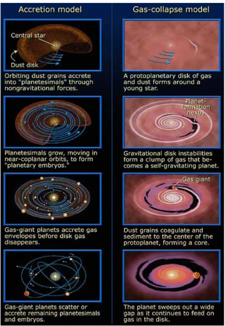
slope of the SEDs change from a positive to negative from Class I to Class III circumstellar disk stages, beyond 10 µm. This image is adapted from Perrot (2017). . . 4 1.3 A schematic diagram illustrating the “core accretion” (Left panel) and the
“gravitational collapse” (Right panel) model, Credits: https://www.nasa. gov/centers/goddard/images/content/96385main_i0319cw.jpg. . . 6 1.4 On the left side, three possible types of orbits are shown. Depending on
the value of beta experienced by the grain, either elliptical, hyperbolic or outward hyperbolic (anomalous hyperbolic) are followed. The image on the right hand side illustrates the elliptical orbits taken by the debris in the parent ring after the collision. Both the images are adapted from Krivov (2010). . . 8 1.5 This image shows a pictorial representation of five zones or belts of a debris
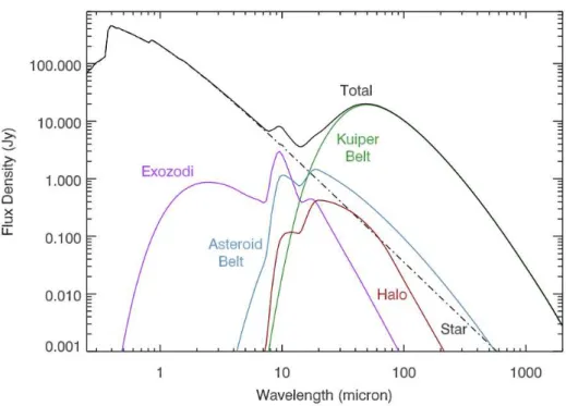
disk detailed Su & Rieke (2014). The five zones are characterized by the temperature of the grains. This representation is based on the solar-system model. . . 9 1.6 The image shows SEDs modeled for different zones of debris disk by Hughes
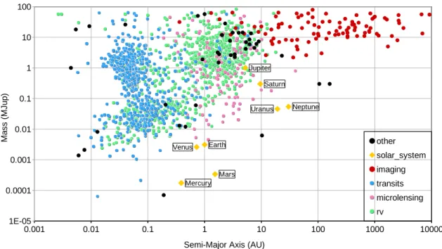
et al. (2018). The models are built around A0V stellar type and are adapted from SEDs of VEGA and β Pictoris. The dotted line represent the emission from the central star. The purple, blue, green, red, and black curves show the emission from the exozodis, the asteroid belts, the Kuiper belt, the halo and the total system (star+disk) respectively. . . 10 1.7 This image plot the mass (MJ) of exoplanets with respect to the semi major
axis represented in AU. This data is collected from http://exoplanet.eu as of August, 2019. The solar system planets are over plotted for reference. 12
1.8 Top: A schematic diagram of an AO system as presented by Rigaut (2015). The correction of the distorted wavefront is performed in real time with the help of a wavefront sensor, a feedback loop and a deformable mirror. Bottom: An image created by distorted wavefront before AO correction (Left) and an image post AO correction (Right) showing the Airy pattern (Sauvage et al., 2016). . . 15 1.9 Top: The image is of the first coronagraph used by Lyot displayed in
Obser-vatoire de Meudon, France. Bottom: Schematic sketch of operation of Lyot coronagraph (Sivaramakrishnan et al., 2001). . . 16 1.10 Top:The image shows debris disk around Fomalhaut as observed by HST (a)
Kalas et al., 2013), Herschel (b) Acke et al., 2012) and ALMA (c) MacGregor et al., 2017). The image in e) and f) show the debris disk around HR 4796 as observed in total intensity by Milli et al. (2017) and in polarimetry in Olofsson et al. (2016). North is up and East is left in all the images and the scale bar is 50 au for the top panel images. The disk is imaged in different wavelengths to see various structural features such as north-east south-west brightness asymmetry in (a), and brightness asymmetry between the two ansae in (b) and 1.3 mm thermal emission map in (c). . . 20 2.1 A top view of SPHERE bench with its sub-systems (IRDIS, IFS, ZIMPOL)
and many opto-mechanical components labelled as seen in Beuzit et al. (2019) 24 2.2 A schematic representation of the ADI technique. Here the disk is in blue
and diffraction from the telescopic optics and the stellar residual are seen in yellow. After subtraction of static speckle pattern (second column) from the science images (first column), each frames are re-rotated (fourth column) and averaged (last column) to obtain a speckle free image. . . 29 2.3 The section of interest (blue) and the section of optimisation (blue)
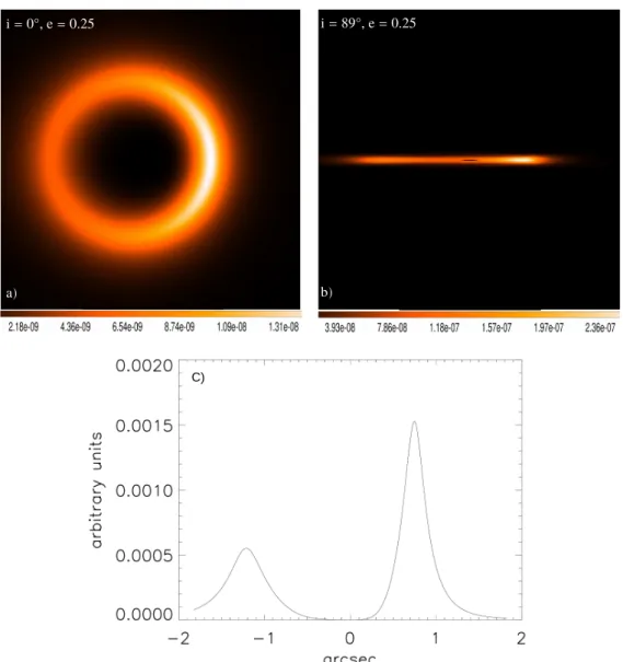
repre-sentation for LOCI. The section of interest (blue) and the section of opti-misation (red) representation for TLOCI as in Galicher et al. (2018) . . . . 30 2.4 a) and b) are the GRaTer images, using the geometrical parameters for
R0 = 100au, h=0.04 and e=0. The FOV of these images are 3.675′′×3.675′′. The colorbar represent the brightness scale of both the images. c) and d) are the plots representing the density variation across the disk corresponding to images a) and b) and normalised to the maximum of the image intensities. 37 2.5 a) and b) are the GRaTer images, using the geometrical parameters R0 =
100 au, αin = 5, αout =−5, i = 89◦ and e = 0. The FOV of these images are 3.675′′× 3.675′′. The colorbar represent the brightness scale of both the images. c) and d) are the plots representing the density variation across the disk corresponding to images a) and b) and normalised to the maximum of the image intensities. . . 38
The colorbars represent the brightness scale in the images. c) is the plot representing the density variation across the disk corresponding to images a) and normalised to the maximum of the image intensities. . . 40 2.7 GRaTer images including both geometrical and phase parameters to
under-stand the affect of g in total intensity and polarimetry for an inclination i=40◦. The FOV of these images is 3.675′′× 3.675′′. The colorbar represent the brightness scale of all the images.. . . 41 2.8 GRaTer images including both geometrical and phase parameters to
under-stand the affect of g in total intensity and polarimetry for an inclination i=80◦. The FOV of these images is 3.675′′× 3.675′′. The colorbar represent the brightness scale of all the images.. . . 42 2.9 Plot of phase functions for different values of g. The solid lines correspond to
polarimetric phase function and the dashed line for the total intensity and the dotted sky blue line corresponds to the combination of 2 g parameters for total intensity. . . 43 3.1 The S/N map of the disk as observed in Asensio-Torres et al. (2016) in
H band. c) is the S/N map of TLOCI reduced image and d) S/N map of the PCA reduced image. Both the images are in [−5σ × 5σ] linearly scale. The arrows point to potential gap at 0.75′′ of north-east side and 0.65′′ at south-west side of the disk. . . 46 3.2 The ALMA 1.3 mm continuum emission is overlaid as white contours as seen
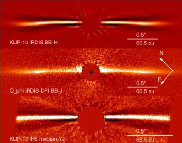
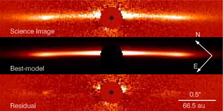
in MacGregor et al. (2018) over the HST STIS images as seen in Schneider et al. (2014) and on the bottom left corner of this image the beam size of ALMA is seen which is about 0.76′′×0.41′′. . . . 47 3.3 Top to bottom: The TLOCI image with front and back side of the disk
labelled, the KLIP image and the Qphi polarimetric image. All the images are rotated to 90◦- PA and cropped at 7′′× 1.3′′. The TLOCI processed, KLIP processed and Qphiimages are scaled linearly between [−1×10−5,1× 10−5]. . . 48 3.4 All the three images of Fig. 3.3 multiplied by the square of the radial scale.
All the images are rotated to 90◦- PA and cropped at 7′′× 1.3′′. All the images are scaled linearly between [0.015,-0.025]. . . 48 3.5 Histograms of Total intensity models with 1 HG (Top) and 2 HG (Middle)
parameter. Bottom: Polarimetric models with 1 HG parameter. Histograms are overlapped with Gaussian when significant . . . 67 3.6 Top:KLIP image of fake-disk injected at 90 ◦ to the real disk. The model
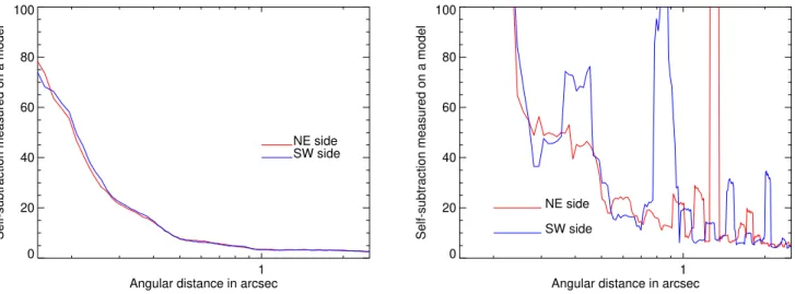
used for fake disk is i=88◦, α
out=-6, αin=2, R0=140 au, g1=0.70, g2=-0.4, w1=0.80, h=0.020, contrast = 0.0005. Bottom: Scaling factor retrieved for the fake-disk compared to its corresponding model . . . 68
3.7 Total Intensity model with the parameters i=88◦, α
out=-6, αin=2, R0=140 au, g1=0.70, g2=-0.4, w1=0.80, h=0.020 convolved with a 2D Gaussian PSF of HWHM=0.37′′. The dark stripes in the ADI processed model (Left) is an effect of ADI self-subtraction. Polarimetric model with parameters i=88.5◦, R0 = 125au, αin= 10.0, αout=-4.0, g=0.8, h=0.020 convolved with a 2D Gaussian PSF of HWHM=0.37′′. . . 69 4.1 The two images correspond to the Fig. B.1 (Leftmost) and B.2 (Top-Left)
from Perrot et al. (2016) respectively. The image on the left shows a bigger FOV with the outer ring, inner ring and associated features. The image on the right shows the IFS FOV with the ring R3 and the clump. . . 73 4.2 On the top row the median image of epoch 1 IRDIS-H2H3 reduced with
KLIP-3 (Left) and TLOCI (Right) is shown. Similarly, on the bottom row the IRDIS-K1 image of epoch 1 reduced with KLIP-3 (Left) and TLOCI (Right) is shown. The features are labelled. The colorbar represents the intensity scale (in arbitrary units) for all images. All the three images are of the FOV 4.97′′× 5.85′′ and smoothed to Gaussian kernel of radius of 5 pixels. . . 76 4.3 Contrast curves extracted with SpeCal for PCA 3 modes reduction of the
epoch 1 (in blue) and epoch 2 (in red) images presented in Fig. 4.2.. . . 77 4.4 Column 1 and Column 2 show the epoch 1 and epoch 2 median image of
KLIP reduced IFS observation, duplicate image of the top panel overplotted with the two ringlets R2 (blue) and R3(green) and the epoch 1 (median image of H2H3 band) and epoch 2 (image of K1 band) of KLIP reduced IRDIS observation overplotted with R2 (blue) and R3 (green). The colorbar represents the intensity scale (in arbitrary units) in all the images. The IFS images are cropped to 1.71′′× 1.33′′. The IRDIS image are cropped to 1.64′′× 1.25′′. All the images are smoothed to a Gaussian kernel of radius of 3 pixels.. . . 78 4.5 Histograms representing the 1% of reduced best-fit model for each
param-eter. Gaussians are overplotted for the histogram corresponding to the in-clination and αin parameters. The . . . 80 4.6 From Left to right: The images show the epoch1 masked KLIP processed
data, the KLIP processed data without the mask, the scaled best-fit model and the residuals map. The green ellipse drawn shows the innermost ringlet R3. The FOV is 0.7′′× 0.98′′ for all the images and smoothed to Gaus-sian kernel of radius of 2 pixels. Colorbar represents the intensity scale (in arbitrary units) for all the images. . . 81 4.7 On left is the image representing the de-projected KLIP 3 modes reduced
IRDIS H2 data. On right is the image representing the de-projected KLIP reduced best-fit model. The colorbar represent the intensity of both the images in arbitrary units. The image is cropped to 2′′× 1.36′′and smoothed to a Gaussian kernel of 2 pixels . . . 82
4.9 The figure represents spectral reflectance corresponding to the northern and southern part of the ringlet R3 in both epochs. . . 85 4.10 The figure represents spectral reflectance plot corresponding to the clump
and the southern part of the ringlet R3 masking out the clump in both the epochs.. . . 85 4.11 The figure (top) shows the three circular masks on the de-projected data
where the red circular region is the clump and the pink dotted circular region encompasses the left and the right regions on each side of the clump.The figure (below) depicts the spectral reflectance at the clump and at circular masks adjacent to the clump (on each side) in both epochs. The dotted lines are the error-bars corresponding to the two other apertures other than that of the clump. . . 86 4.12 Fitted synthetic spectra to the reflectance spectrum of epoch2. The dotted
line represents the best-fit spectra with smin = 0.30 µm and κ = -3.00 and the dashed line represent the spectra for fiducial case where smin = sblow and κ = -3.5. . . . 88 4.13 Debris disk around HD 106906 AB from Kalas et al. (2015) (Left) and an
arrow pointing to the planet HD 106906 AB b at 7′′ as seen in Lagrange et al. (2016) (Right). In both the images, north is up and east is left. . . 90 4.14 The topmost image is the KLIP-5 science image of HD 106906 as observed
by IRDIS BB_H. The image in the middle row is the IFS median image of the debris disk and the polarimetric Qϕ image of the disk smoothed to a Gaussian kernel of radius of 2 pixel is in the third row. . . 94 4.15 The disk and the thirteen point-sources encircled in green within the IRDIS
FOV is presented in the top row. The white arrow indicates the already known planet. In the bottom row a plot of the contrast of the planet in IRDIS BB_H filter is presented. . . 95 4.16 The histograms of total intensity models and polarimetric models are
pre-sented in the bottom two and top two rows respectively. Histograms are overlapped with Gaussian functions unless the distribution is continuously increasing or decreasing. . . 100 4.17 Left image from top to bottom presents the KLIP 5 IRDIS BB_H image,
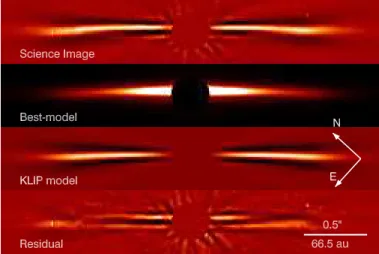
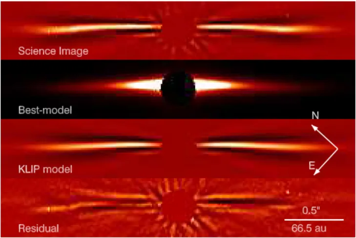
the total intensity best-fit model convolved with the instrumental PSF, the corresponding reduced best-fit model and the residual. The science image, reduced best-fit model and the residual image are scaled linearly between [−1 × 10−5,1 × 10−5] and the best-fit model convolved with the instru-mental PSF is scaled linearly between [0.0,0.5].image from top to bottom presents the Qphiimage, the polarimetric best-fit model convolved with the instrumental PSF and the residual. All the three images are scaled linearly between [−4 × 10−7,4 × 10−7] . All the images are rotated to 90◦-PA and cropped to 2.85′′× 0.5′′. . . . 101
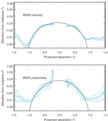
4.18 The surface brightness profile in total intensity (Left) in BB_H filter and polarimetry (Right) in BB_J filter. . . 101 4.19 The spectral reflectance plot with a positive slope of 0.0012 contrast/arcsec2
in NIR YJH bands . . . 102 4.20 Best fits of the reflectance spectrum obtained for a fiducial case with smin =
sblow and κ = −3.5 (left), and for best-fit when smin and κ are free param-eters (right). . . 103
List of Symbols
Fλ Flux distribution in SED
λ Wavelength
D Diameter of the focal plane of telescope ⃗
Fg Stellar gravitational force
⃗
Frad Radiation pressure ⃗
Fdrag Drag force
G Gravitational constant m Mass of grains in debris disk M∗ Mass of a central star M⊕ Mass of the Earth
r Radial distance in disk coordinates ⃗
er Radial unit vector
β The ratio between the radiation pressure and the gravitational force ⃗
Fpg Photogravitational force e Orbital eccentricity ρ Bulk density of grains s Grain size in debris disk
sblow Blowout size of the grains in debris disk
dn Particle size distribution of the grains in debris disk κ Power law index of particle size distribution
fIR Fractional luminosity of the disk L∗ Stellar luminosity
LIR Disk’s luminosity Td Disk temperature
I Master cube of science images observed with SPHERE A Image of static speckle pattern
IADI Image after speckle pattern is subtracted from science image Θ Parallactic angle
i, j Spatial axis of the master cube l Index of temporal axis
If Final image after speckle correction, re-rotation and averaged N Total number of angular frames
n Sections of image used for post-processing with LOCI technique ϱl Area of the sections n
lw Index or temporal axis in the sections n
I′ Speckle pattern calculated using LOCI or TLOCI techniques in different sections of the science image
clw Coefficients computed by LOCI
b combination of the spatial axis i, j Inorm Normalized science images xxii
P C Principle components calculated during KLIP technique
T Transpose of a vector
I, Q, U, V Stokes vectors
Q+, U+, Q−, U− Modulated set of images representing the Stokes vector IL0, IL22.5, IL45, IL67.5 Images obtained in the left channel in four polarisation angle IR0, IR22.5, IR45, IR67.5 Images obtained in the right channel in four polarisation angle
ϕ Azimuthal angle with respect to center of the star Qphi, Uphi Azimuthal stokes vector
ν Degree of freedom in χ2 calculation
Si,j Science image
Mi,j Reduced model
Ndata Total number of pixels in the region of interest where χ2 is calculated Nparams Number of parameters used to create a GraTer model
a Scaling factor between two arrays
G Distribution function in GRaTer
H Scattering phase function
ρG Density distribution function in GRaTer
z Distance to the midplane
g Anisotropic scattering function
θ Scattering angle
ρ0 Density on the midplane
R0 Distance where the density of the parent ring peaks
γ Power law of the exponential function in the density distribution βf Radial flaring index of a disk
ζ0 Vertical thickness of the disk at different radial distance
h Scale height of a disk
αin, αout Positive and negative power law indices of the radial distribution fT I Henyey Greenstein phase function
i Inclination of the disk
xd, yd, zd The disk coordinates
θ∗ The angle between xdand yd axes
fP Polarised phase function
P Porosity of grains in debris disk
CHAPTER
1
Introduction
1.1 From molecular clouds to stellar systems . . . . 2
1.2 From planetesimals to planets . . . . 3
1.3 Debris Disks . . . . 5 1.3.1 Physics behind debris disk. . . 7
1.3.2 Debris disk architecture . . . 9
1.3.3 Detection of Debris disk with Infrared Spectroscopy and SED . . 10
1.4 Observation of exoplanets . . . 11 1.4.1 Radial velocity method . . . 11
1.4.2 Transit method . . . 12
1.4.3 Microlensing . . . 13
1.4.4 Direct Imaging of exoplanets . . . 13
1.5 Imaging debris disk . . . 18 1.5.1 Thermal Imaging . . . 18
1.5.2 Scattered Light Imaging . . . 18
1.6 Motivation . . . 19
1.7 The course of this thesis . . . 21
Looking up at the night sky, we see millions of twinkling stars with naked eyes. In reality, there are billions of such stars in the universe. These are classified according to their properties such as stellar luminosity, surface temperature, age, mass, and size. Because of such diversity astronomers look for and study various types of stars to understand stellar evolution. In January 1983, the Infrared Astronomical Satellite (IRAS) was launched to survey the sky in far-infrared wavelengths. The first task of this satellite was to calibrate the detectors which had to be done by observing a few bright stars whose properties were thought to be well understood at that time. One such star observed was Vega, which is an A0 type star in the Lyra constellation. The blackbody spectrum of the star can be used to calculate the temperature of the star and Vega was often taken as a point of reference for astronomical objects to be scaled in magnitude. Therefore, Vega was one of the primary targets of IRAS. As soon as the spectrum of the star was generated, it was seen that there was an excess response at long wavelengths. This was a perplexing result and immediate
2 1.1 From molecular clouds to stellar systems measurements of multiple such stars were obtained. It was soon realized that there was no instrumental issue with IRAS but this excess emission was from a cold dust-gas region at a distance of several astronomical units away from the stars. These emissions were from the circumstellar disks around their respective central stars.
The infrared excess emission of Vega opened a new class of study dedicated in the search of stellar systems or exosystems with a circumstellar disk around their central star. While on this quest, many stellar systems have been discovered which has helped our understanding of the formation and existence of our solar system. The solar system itself is an outcome of star and planet formation. To be precise, it is the final stage of the circumstellar disk to planet evolution. This thesis focuses on one of the intermediate steps between star to planet formation and that is the debris disk stage. This class of disk is the last stage of a circumstellar disk and a precursor of solar system. Observing such disks and possible planets within such systems can not only open gateways to finding life signatures but also tell more about the past of solar system. Thus, current and future telescopes are going leaps and bounds to detect debris disks where planet-forming signatures or an Earth-like exoplanet can be found.
1.1 From molecular clouds to stellar systems
Young stellar environments are formed within the cold and dense regions of the interstellar medium (ISM) known as molecular clouds. The schematic illustration of the stellar system evolution process is given in Fig.1.1. Molecular clouds are made up of gas-dust mixture and are gravitationally unstable. The primary constituent (∼90%) of these clouds is molecular hydrogen (Krumholz,2011). However, over 150 types of chemical constituents, including He and CO have been detected in their gaseous form in the molecular clouds. The dust present in these clouds is stellar remnants mostly consisting of silicates and carbonaceous sub-micron grains. At this stage, the cloud is optically thin with regions of density of 104-106 cm−3 (Fig. 1.1(a)) and temperature ∼10 K. In a few thousands of years, the density in these regions increases under the influence of gravitational collapse overpowering the gas pressure and the magnetic forces. This forms a “Class 0” stage with an optically thick core inside an envelope as seen in Fig.1.1(b). The source of such dense cores is undetectable between the visible and mid-infrared (mid-IR) wavelengths because of the optical thickness and the low temperature (Hueso & Guillot, 2005; Yorke et al., 1993).
The accretion of the dense core starts to form the central protostar. The protostellar system is fed by the overlying envelope making this envelope thinner compared to that of its Class 0 counterpart. The high angular momentum of the dense core is vastly transported in forming a circumstellar disk surrounding the protostar. The transport of the angular momentum of the system is balanced by powerful out driven bipolar jets. The protostar, the surrounding disk, the remaining envelope, and the bipolar jets together form the “Class I” stage of the stellar system evolution (Fig.1.1(c)).As gas and dust are transported inward through the disk onto the protostar, massive amounts of materials are ejected out of these lobes at a velocity of several hundreds of kilometers per second (Ollivier et al.,2009).The excess emission from the disk can be detected in the spectral energy distribution (SED)
over the black body curve followed by the protostar. SED describes the distribution of the energy in terms of λFλ of a system as a function of wavelength. The power-law slope
of the SED of Class I objects is positive (Armitage,2019) compared to a pure star that follows Rayleigh-Jeans law as seen in Fig.1.2. The Class I stage remains for ∼105 years.
The envelope around the protostar of Class I stage completely dissipates slowing down the accretion rate of the young stellar system. At this stage, the power-law slope of the SED becomes negative as seen in Fig.1.2. However, it still has a significant excess above the Rayleigh-Jeans curve followed by the central star and is classified as “Class II” (Fig. 1.1(d)). Class II lasts up to a few million years. The disk around the central star is known as the protoplanetary disk as seen in Fig. 1.1(d). The material within the protoplanetary disk continues to fuel the stellar accretion and the outflow. How-ever, simultaneously, the dust grains and gas start processing to form planetesimals and protoplanets.
The process of protoplanet formation accretes the gas present in the protoplanetary disk and leaves behind the protoplanets and the debris of planetesimals. This leads to a “Class III” phase (Fig. 1.1(e)) where the power-law slope of the SED is steeper than the Class II phase but still has some amount of excess (Fig.1.2). The optically thin disk around the star is known as the debris disk. As planet cores and giant planets are expected to have already formed in this stage, they continuously collide and form smaller grains that survive in a debris disk. So this type of disk is not the leftover of a protoplanetary disk, rather they are the leftover of already formed planets (Hughes et al., 2018; Kral et al., 2016). With time, the disk loses its mass due to the formation and evolution of a planetary system as shown in Fig. 1.1(f). Evidence suggests that the Kuiper belt in our solar system is the remnant of a massive debris disk. Following this analogy, a stellar system with a debris disk can be considered as an immediate precursor of our star-planet system. This thesis concerns the study of debris disks formed around Class III objects. Details on the fundamentals of debris disk formation, their architectures and the physical processes involved are described in Sect.1.3.
1.2 From planetesimals to planets
A sufficient amount of sub-micron dust and gas from the ISM is sustained during the evo-lution of circumstellar disks. Though there exist several theoretical models of explaining the evolution of planets, it is generally accepted that young planets are formed during the protoplanetary disk phase. Below, I briefly explain the two most established theories: core-accretion and gravitational instability.
• Core-accretion (Pollack et al., 1996; Rice et al., 2003): The sub-micron sized dust grains stick together to form centimeter-sized particles. Increasing size of grains force them in settling towards the disk mid-plane (Blum & Wurm,2008;Dullemond & Dominik, 2008;Zsom et al., 2010). Goldreich & Ward (1973) proposed that the kilometer-sized planetesimals are formed when the clumps of meter-sized particles directly collide with each other. This stage can be of complex dynamics as there can be elastic collision (Booth et al.,2018), radial drifts of metric particles towards
the star (Laibe et al.,2012) and/or fragmentation of these particles during collisions instead of coagulation (Gonzalez et al.,2017). The planetesimals, under the grav-itational influence, grow to form terrestrial planets or massive planetary cores for gaseous planets at outer orbits. Once these planetary cores have become sufficiently massive ( 10-20 M⊕ ), they accrete gas from the disk to form giant planets.
The limitation of this model is the timescale of the planet formation. Protoplanetary disks generally survive up to 5 Myr whereas, the core accretion process creating giant planets would require ∼10 Myr. The timescale of planet formation can be reduced by planetary migration. Evidence of planets younger than 10 Myr has already been found (e.g. PDS70b, Keppler et al., 2018). Under the influence of the negative torque produced by the gas, a planet would move inward. This process would lead to an accretion of a higher amount of gas and dust by the planet in much shorter timescale (Alibert et al.,2005).
• Gravitational instability (Boss, 2002; Cameron, 1978): This model is a “top down” route for planet formation in protoplanetary disks. According to gravitational insta-bility, in massive and cold protoplanetary disks, dense gaseous regions are formed and they collapse under the influence of self-gravity. This collapse continues and forms a self-gravitating gas giant. The core of the planet is formed after the collapse, by the coagulation of dust from the disk carving out wide gaps. The planet formation in this process takes 1 Myr which is less than the core accretion model. Additionally, more distant planets can be formed by gravitational instability as compared to the core-accretion model where the planet formation is limited to 10-30 au. However, the limitation of this model is having a cold and massive protoplanetary disk as a prerequisite.
Figure 1.3 show a schematic diagram of the possible steps involved in core-accretion and gravitational instability models. These two models are widely accepted theories of planetary evolution in the scientific community. With more and more observational data, planet formation theories are evolving. Studying circumstellar environments is helping us constrain the stellar system evolution and planet formation theories. As debris disks are considered to be the evolved form of circumstellar disks where planet formation has already started, studying these disks can provide important clues about planet-disk-interactions in stellar environments. In the next section, details regarding the physical processes, architecture, and detection techniques using SED of such disks are provided.
1.3 Debris Disks
About 20 % of nearby main sequence stars have debris disk around them. As defined in Sect.1.1, these disks are the type of circumstellar disk which reaches “Class III” phase after planetesimals and giant planets have already been formed and believed to have accreated most of the gas in the system. The planetesimals continuously collide to form small grains and these small grains collide amongst each other to form sub-micron grain. This process of continuous grinding of grains in a thin belt is known as collisional cascade(Hughes et al., 2018). Debris disks are reservoirs of varied sized grains which depending on the size emit at different wavelengths (Sect.1.3.2). Since these grains are mostly produced by secondary
6 1.3 Debris Disks
Figure 1.3 – A schematic diagram illustrating the “core accretion” (Left panel)
and the “gravitational collapse” (Right panel) model, Credits: https://www.nasa. gov/centers/goddard/images/content/96385main_i0319cw.jpg.
processes the disk itself is called a secondary disk. The primary forces which act on such grains within a debris disk are the gravity of the central star ⃗Fg, the radiation pressure from the central star ⃗Fradand the drag forces ⃗Fdrag. The effects of these forces are detailed in Sect.1.3.1.
Apart from the presence of different types of dust grains in debris disks, recent observa-tions by Atacama Large Millimeter Array (ALMA) have shown that a significant amount of gas is present in these disks (Kral et al.,2018;Moór et al., 2017). These observations contradict our previous understanding of debris disks that were known to have a much lower gas to dust ratio. This gas tends to affect the drag forces experienced by the grains which are discussed in Sect.1.3.1.
1.3.1 Physics behind debris disk
The radiation pressure ( ⃗Frad) of the central star exerts an outward force that is respon-sible for blowing smaller grains out of the system (Burns et al., 1979). The net force of radiation pressure and stellar gravity ( ⃗Fg) experienced by the grains is known as the “photogravitational” force. This is given by ⃗Fpg as detailed inKrivov (2010).
⃗
Fpg = ⃗Fg+ ⃗Frad =−
GmM∗(1− β)
r2 e⃗r, (1.1)
where G is the gravitational constant, m is the mass of the grain located at distance r from a central star of mass M⋆, ⃗er is the radial unit vector and β is the ratio between
the radiation pressure and gravitational force such that β =
F⃗rad/ ⃗Fg
. β is inversely proportional to the grain size s and the grains bulk density ρ. This parameter classifies the orbits assumed by the dust grains. When 0 ≤ β < 0.5, the grains follow a circular (β = 0) or elliptical orbit (0 < β < 0.5) and are “bound” to the system. If 0 < β < 0.5, the grains follow eccentricity orbit where the eccentricity is given by e = β
1− β. When β = 0.5, the “blowout size” sblowlimit is set, which is the minimum size needed for a grain to be able to stay bound to the system. If 0.5 < β < 1, the grains become “unbound” and are blown out of the system following either a parabolic (β = 0.5) or a hyperbolic (β > 0.5) orbit. Finally, for β > 1.0 the gravitational force is overwhelmed by the radiation pressure. As a result, such grains follow a non-Keplerian trajectory defined by “anomalous hyperbola” which moves the grains outward from the release point. Figure 1.4 (Left) illustrates the cases of β with different values and the corresponding orbital trajectory followed by the grains. When β is within the range of 0.0-0.5, the grains are segregated according to their sizes in different orbits. Since β is inversely proportional to the grain size s, a higher value of β corresponds to smaller grains and because the effect of radiation pressure is stronger on smaller grains, such grains tend to move to a larger orbit. Figure 1.4 (Right) shows that the size of the orbit increases with an increasing value of β within the range of 0.0-0.5. The particle size distribution is often described dn(s) ∝ sκds where κ is the
power-law index. For the debris disk to be stable, there exist a balance between the grain loss due to radiation pressure and an increase in the production of such grains by a collisional
8 1.3 Debris Disks
Figure 1.4 – On the left side, three possible types of orbits are shown. Depending
on the value of beta experienced by the grain, either elliptical, hyperbolic or outward hyperbolic (anomalous hyperbolic) are followed. The image on the right hand side illustrates the elliptical orbits taken by the debris in the parent ring after the collision. Both the images are adapted fromKrivov (2010).
cascade. This state is known as the “quasi-steady state” where the power-law index is −3.5 Dohnanyi (1969) for the particle size distribution within the debris disk. Most current models identify κ to be in between -3.0 to -4.0.
The drag forces, in general, tend to affect the grains in a way such that they move inward within the system. In the context of a debris disk, these forces include Poynting-Robertson (PR) effect and gas drag. The PR effect is caused due to an orthoradial component of the stellar radiation pressure (Kral et al.,2016). As a result, this force acts opposite to the radiation pressure and millimeter-sized grains spiral towards the central star. Wyatt (2005b) described that under the effect of grain-grain collision in case of massive debris disks, millimeter-sized grains would break into much smaller pieces before migrating further in towards the star. Consequently, the effect of PR drag is very small for most observed debris disks. Another drag force that plays an important role is the Epstein force (Takeuchi & Artymowicz,2001). This effect is due to the presence of gas in the disk. Some theories predict that the gas present in these systems can interact with the grains and affect the morphology of the disk when the gas-to-dust ratio is close to unity. For example, Lyra & Kuchner (2013) discussed the formation of gaps in the presence of gas when the gas-to-dust ratio is close to unity without taking into account the formation of planets. The presence of gas can also explain the presence of small grains below the blowout size in the disk (Bhowmik et al.,2019).
Other forces, such as the magnetic fields creating clumps (Rieke et al.,2016;Su et al., 2016), sublimation of larger grains while undergoing PR drag (e.g.Kobayashi et al.,2009), eccentric planet perturbing the disk’s eccentricity (Wyatt et al.,1999), etc can influence the disk’s chemistry and geometry.
Figure 1.5 – This image shows a pictorial representation of five zones or belts of
a debris disk detailed Su & Rieke (2014). The five zones are characterized by the temperature of the grains. This representation is based on the solar-system model. 1.3.2 Debris disk architecture
New development in the field of debris disk theory and observation has led to constrain the architecture of such disks. Debris disks are often comprised of multiple belts (Kennedy & Wyatt, 2014). Based on the solar system model, five zones of debris disk has been proposed bySu & Rieke (2014) as seen in Fig.1.5. The classification of different zones is based on the temperature of the grains present in that particular zone. The most easily observable part of the disk is the outer part which has dense cold grains with ∼ 50 K temperature. The dust grains mostly emit in the far-IR wavelengths. This is analogous to a massive form of “Kuiper belt” of our solar system (Carpenter et al.,2009). The dust mass is expected to be between 100− 103 M⊕. Many disks consist of a warm component (100-200 KBallering et al., 2013; Moór et al.,2009; Morales et al., 2012) comparable to the present asteroid belt of our solar system. The dust grains in the warm belt emit at mid-IR wavelengths. The mass of such disk is estimated byKrivov(2010) to be in between 10−8− 10−6 M⊕. Broadly, it can be said that multiple parent belts can be present in a debris disk which consists of the warm and cold component. Beyond the Kuiper-belt zone there is expected to be a disk halo of smaller dust grains (e.g.Schneider et al.,2014).
The terrestrial zone which is populated with larger grains is at a closer separation from the central star. This zone on closer inspection can probe certain features associated with rocky planet formation, such as grain crystallization and/or Moon-forming impact (Lisse
10 1.3 Debris Disks
Figure 1.6 – The image shows SEDs modeled for different zones of debris disk by
Hughes et al.(2018). The models are built around A0V stellar type and are adapted from SEDs of VEGA and β Pictoris. The dotted line represent the emission from the central star. The purple, blue, green, red, and black curves show the emission from the exozodis, the asteroid belts, the Kuiper belt, the halo and the total system (star+disk) respectively.
et al., 2009; Mittal et al., 2015). At a very close distance of 1 au, exozodiacal dust or sometimes referred to as “exozodis” of temperature ∼1500K have been detected.
This scheme is largely inspired by the solar system model. However, observations of exoplanets have taught us that the solar system model might not be an ideal paradigm to describe all debris disks. Therefore, further observations of different types of debris disks would constrain our understanding of the grain distribution within debris disks and their architectures.
1.3.3 Detection of Debris disk with Infrared Spectroscopy and SED Historically, the most immediate way of detecting a debris disk is to obtain its SED. The dust grains in the disks are heated by the stellar radiation, which emit to show an IR excess mostly in 10-170 µm. The debris disk around Vega was the first disk detected by the IR excess using IRAS (Infrared Astronomical Satellite,Aumann et al.,1984). Over 500 nearby debris disks are observed by Spitzer Space Telescope, ISO (Infrared Space Observatory) and Herschel (Chen et al.,2019). The most important physical parameter obtained from these observations is the fractional luminosity of the disk given by fIR = LIR/L∗, where, LIRand L∗ are the disk and stellar luminosity respectively. Here, the disk luminosity can
either be calculated by integrating the disk flux from the SED or the maximum of the flux and the corresponding wavelength in the SED (Wyatt,2008). The temperature of the grains in the disk can also be calculated using Wien’s displacement law.
Some SEDs studied byMorales et al.(2011) showed a bimodal distribution of temper-ature (a cold Td ∼ 50 K and warm dust component Td ∼ 200 K) which can be explained by multiple zones or belts in the debris disk. In Vega (Absil et al., 2006) and τ Ceti (even warmer, di Folco et al., 2007) exozodiacal dust has been inferred from the SED. SEDs modeled byHughes et al. (2018) for multiple belts in a debris disk is illustrated in Fig. 1.6. The illustrated SED is adapted from the models of Vega and β Pictoris debris disk. The model is built for an A0V star, 7.7 pc away with a total integrated luminosity of 1.4×10⁻³.
Apart from the calculation of fractional luminosity and disk temperature, features associated with terrestrial events can also be inferred. Silicate features at 10µm can be extracted which can be indicative of grain growth and crystallization (e.g.Bouwman et al., 2001). In a few other cases, spectral features such as Fe-rich sulfides feature, water ice feature, etc, are also detected (e.g.Lisse et al.,2007).
Current observations of debris disks are continuously changing and challenging the known theories of debris disks. For example, the presence of massive amounts of gas led us to integrate a gas drag in the influential forces experienced by grains within a debris disk. Also, the detection of giant planets at a very close distance from the star made us realize that the solar system model for debris disk architecture might be a special case and not a general representation. The most recent developments in theories of debris disks have come from the detection and resolving of exoplanets. As a result, exoplanet and debris disk studies have become complementary to each other. Hence, in the upcoming sections, I am briefly explaining a few techniques to observe exoplanets and debris disks.
1.4 Observation of exoplanets
An exoplanet is a planet that orbits a star other than our Sun. Over the past two decades, several thousands of exoplanets were detected by different techniques. The most commonly known methods are radial velocity, transits, microlensing, and direct imaging. As of 30th
of August 2019, we have confirmed the detection of 4,110 exoplanets by the existing techniques described below. Apart from these confirmed discoveries, about 2,500 planet candidates are yet to be confirmed. The plotted data in Fig. 1.7 shows the distribution of exoplanets detected by various indirect and direct methods in terms of mass and semi-major axis, which are briefly explained below.
1.4.1 Radial velocity method
One of the oldest methods to detect exoplanets is by identifying a Doppler shift in the stellar spectrum due to the gravitational pull of the planet. When a planet with significant mass orbits its star, the star acquires a periodic motion and rotates about the center of
12 1.4 Observation of exoplanets
Figure 1.7 – This image plot the mass (MJ) of exoplanets with respect to the semi major axis represented in AU. This data is collected from http://exoplanet.euas of August, 2019. The solar system planets are over plotted for reference.
mass of the system. By monitoring the perturbation in the radial velocity of the star, the minimum mass, eccentricity and the orbital period of the planet can be calculated. This calculation is possible only when Keplerian orbits are assumed. However, this technique is most sensitive to planets with a small orbital period in between 0-5 au (peaking at 1 au) and, like “Hot Jupiters” (masses greater than 100 M⊕) and “super-Earths” (3-30 M⊕), as seen in Fig. 1.7. A limitation of this technique is the underestimation of the planetary mass when the orbital plane of the planet is not aligned to the line of sight of the observer.
1.4.2 Transit method
In this technique, the dimming of starlight is observed when a planet passes in front of its star. To successfully find a planet using transit, the orbital plane of a planet should be aligned with the line of sight of an observer. The periodic dimming of starlight determines the planet’s mass and radius (Ollivier et al.,2009). Moreover, the spectrum of a planetary atmosphere can be studied using this technique. Apart from the alignment requirement, the detection of transiting planets is sensitive to short-period planets. However, owing to space missions such as KEPLER/K2 and TESS (Ricker et al., 2015) the number of exoplanets discovered and validated by this technique has largely increased as seen in Fig.1.7. With 2,954 planets detected until August 2019, the transit method has been the most successful technique among all the other methods.
1.4.3 Microlensing
The microlensing technique detects planets based on the phenomenon of a gravitational lens that creates an effect of magnification (Einstein, 1936). When a massive object is present between the observer and the source, the image of the source is deformed and magnified. In the case of microlensing, distortion of starlight of a background star due to a source star with an exoplanet in the foreground is detected and associated with the planet detection. This technique has an advantage as it can detect less massive planets and/or planets with an orbital period of more than a few hundred days. This trend can be seen in Fig1.7where super Earth-type planets are detected. The biggest drawback to this technique is that the microlensing events are extremely rare and never repeat for the same target.
1.4.4 Direct Imaging of exoplanets
Direct imaging, in contrast to the above-explained indirect methods, obtains the image of the planets. The goal of obtaining the image of an exoplanet is to measure its flux, obtain a spectrum and determine its orbit. The exoplanet candidates which are point sources can either be detected in reflecting light (at visible wavelengths) or in its thermal emission (at IR wavelengths). While indirect observations have proven quite effective in exoplanet detection, direct imaging technique offers complimentary advantages.
This technique gives access to the spectro-photometric and possibly polarimetric mea-surements of planet atmospheres. Spectral information can determine certain key param-eters, such as the temperature, surface gravity, the presence of certain molecules such as methane or water, cloud fraction, the mass of the planet, etc.. However, atmospheric and planet formation models are mandatory to interpret such data. Also, in just a few epoch observations, orbital characterization of the exoplanet can be done by direct imaging. Also, images of young stellar systems can be obtained. These observations can detect planets at a very young age before migration takes place. This way the technique can potentially put a constraint on planet formation. Another major advantage of this technique is the possibility to capture an entire stellar system at once. Therefore, in principle a system with multiple planets, exo-moons and a circumstellar disk can all be detected. These observations have led to a better understanding of circumstellar disk evolution. Direct imaging, however, is quite challenging because of two requirements.
1. The star-planet contrast: The flux ratio, Fp/F∗, of an Earth-Sun system with an
angular separation of 0.5′′ at 10 pc is 10−10 in the visible range. For a Jupiter-Sun system, it is 10−9 (Traub & Oppenheimer,2010). As flux is wavelength-dependent the flux ratio for an Earth-like planet will lie in between 10−8 to 10−7 at 0.1′′ in the IR, which is still non-achievable with current ground-based high-contrast imagers. 2. The star-planet angular resolution: The second challenge is to observe an exoplanet
at small separations. A planet of interest (exo-earth or super-Earth) would lie be-tween 0.1-0.5′′. However, 30 plus meter class telescopes are expected to observe terrestrial planets. From space, imaging terrestrial planets around Sun-like star
14 1.4 Observation of exoplanets would still need greater than 4 meter class telescopes. Using such monolithic tele-scope can induce launching limitations. However, segmented mirrors in teletele-scopes as used in JWST (James Webb Space Telescope) is the next advancement to this technology.
Because of the two challenges, until now there are only a handful of exoplanets that are directly imaged, as seen in Fig.1.7. The most observed planets are giant planets at large separations known as EGP (Extrasolar Giant Planets) which is because of the current challenge faced by imaging from both space (Hubble Space Telescope) and ground.
The requirement to achieve high contrast is challenging, firstly wavefront errors are always present and secondly, the stellar glare infiltrates the image which incapacitates observation of faint exoplanets. Wavefront aberrations can occur in space-based observa-tion due to optomechanical vibraobserva-tions. And for ground-based observaobserva-tions, the Earth’s atmosphere introduces turbulence. This turbulence adds to the wavefront aberrations, degrading the image quality. To solve this issue an AO (Adaptive Optics,Babcock,1953) system is used to correct for the aberrations induced by the turbulence. Similar tech-niques are required for space-based observations. Secondly, to suppress the starlight or the diffraction effect of a telescope an optics called coronagraph is used. In this thesis, such a ground-based instrument including these techniques are used. Thus, these techniques are explained in the forthcoming subsections.
1.4.4.1 Adaptive optics
The light from a stellar object is emitted in the form of a spherical wave. Traveling a quasi-infinite distance to the Earth these spherical waves are treated as plane waves and ideally should form an “Airy Disk” diffraction pattern (Point Spread Function or PSF) at the telescope’s focal plane. When limited by diffraction, the angular resolution of a telescope is given by λ/D where D is the diameter of the entrance pupil of the telescope. However, atmospheric turbulence distorts the wavefront at the entrance pupil and degrades the angular resolution. The distortions are dominated by phase fluctuations and have comparatively small amplitude fluctuations. These fluctuations produce residuals known as speckles in the images. These speckles can be misidentified as planet signals in the science images. Therefore it is necessary to correct for such distortions. The distorted wavefront can be corrected in real-time with AO, to approach the theoretical diffraction limit.
The atmospheric turbulence-control requires three steps: measurement of the wave-front distortion, calculation of the necessary correction and application of the correction to the incident wavefront. The diagram of a conventional AO system is presented in Fig.1.8 (Top). The incident light from the source is divided into two paths using a beam-splitter, one of them sends the light towards a wavefront sensor and the other towards the camera. The distorted wavefront is then measured by a wavefront sensor and a real-time calculator determines the shape to be applied on the deformable mirror to compensate for wavefront phase errors (Madec,2012). The AO system works in a closed-loop.