Beyond normality: Learning sparse probabilistic graphical models in the non-Gaussian setting

Figure 20: Cholangiographie rétrograde endoscopique montrant la présence du matériel hydatique dans la voie biliaire principale ;. Figure 21 : Cholangiographie rétrograde

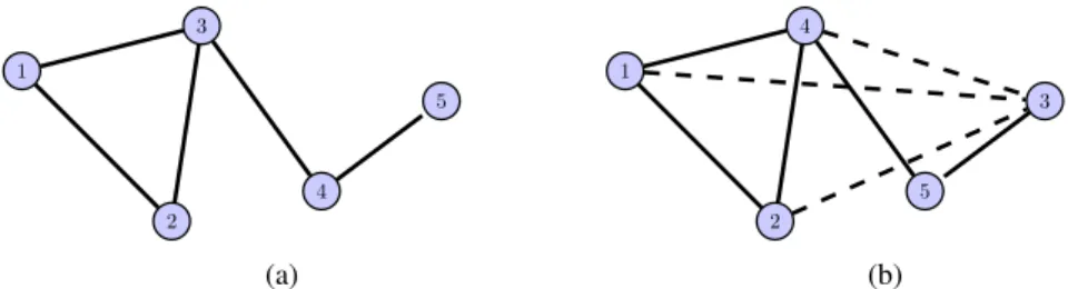
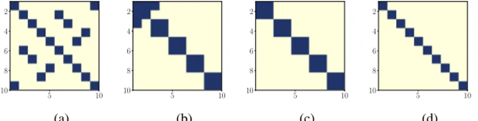
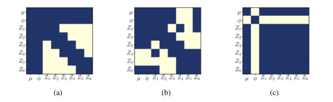
Si les graphes des modèles graphiques non orientés sont caractérisés par les zéros de la matrice de précision, les propositions qui suivent lient le graphe d’un modèle

It is an important step for statistical physics since the authors are able to show by explicit calculations that, in two examples of random variables, previously put forward

tau xi precuneus hippocampus entorhinal cortex fusiform gyrus midtemporal lobe amygdala temporal pole insula parahippocampus cortex ventricles ADAS-Cog (multi-domain) RAVLT

Dis autrement, cette deuxième étape consiste donc en une analyse en profondeur de la relation de causalité entre (a) le changement de régime institutionnel

Keywords: Estimator selection, Model selection, Variable selection, Linear estimator, Kernel estimator, Ridge regression, Lasso, Elastic net, Random Forest, PLS1

We first investigate the order of magnitude of the worst-case risk of three types of estimators of a linear functional: the greedy subset selection (GSS), the group (hard and

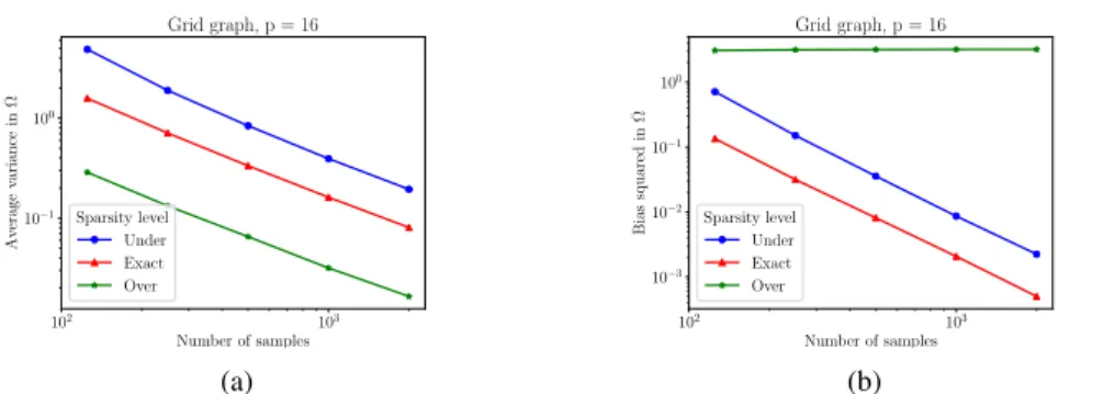
Recalling that most linear sparse representation algorithms can be straight- forwardly extended to non-linear models, we emphasize that their performance highly relies on an

References

[1] D. Bigoni, A. Spantini, and Y. Marzouk. On the computation of monotone transports. In preparation. [2] V. I. Bogachev, A. V. Kolesnikov, and K. V. Medvedev. Triangular transformations of measures. Sbornik:
Mathematics, 196(3):309, 2005.
[3] T. Cai and W. Liu. Adaptive thresholding for sparse covariance matrix estimation. Journal of the American Statistical Association, 106(494):672–684, 2011.
[4] J. Friedman, T. Hastie, and R. Tibshirani. Sparse inverse covariance estimation with the graphical lasso. Biostatistics, 9(3):432–441, 2008.
[5] S. K. Ghosh, A. G. Cherstvy, D. S. Grebenkov, and R. Metzler. Anomalous, non-Gaussian tracer diffusion in crowded two-dimensional environments. New Journal of Physics, 18(1):013027, 2016.
[6] S. Kim, N. Shephard, and S. Chib. Stochastic volatility: likelihood inference and comparison with ARCH models. The Review of Economic Studies, 65(3):361–393, 1998.
[7] H. Knothe. Contributions to the theory of convex bodies. The Michigan Mathematical Journal, 1957(1028990175), 1957.
[8] D. Koller and N. Friedman. Probabilistic Graphical Models: Principles and Techniques. MIT Press, 2009. [9] C. Liu, R. Bammer, B. Acar, and M. E. Moseley. Characterizing non-Gaussian diffusion by using
generalized diffusion tensors. Magnetic Resonance in Medicine, 51(5):924–937, 2004.
[10] H. Liu, F. Han, M. Yuan, J. Lafferty, and L. Wasserman. High-dimensional semiparametric Gaussian copula graphical models. The Annals of Statistics, 40(4):2293–2326, 2012.
[11] H. Liu, J. Lafferty, and L. Wasserman. The nonparanormal: Semiparametric estimation of high dimensional undirected graphs. Journal of Machine Learning Research, 10:2295–2328, 2009.
[12] P.-L. Loh and M. J. Wainwright. Structure estimation for discrete graphical models: Generalized covariance matrices and their inverses. In NIPS, pages 2096–2104, 2012.
[13] Y. Marzouk, T. Moselhy, M. Parno, and A. Spantini. Sampling via measure transport: An introduction. In R. Ghanem, D. Higdon, and H. Owhadi, editors, Handbook of Uncertainty Quantification. Springer, 2016. [14] N. Meinshausen and P. B¨uhlmann. High-dimensional graphs and variable selection with the lasso. The
Annals of Statistics, pages 1436–1462, 2006.
[15] T. A. Moselhy and Y. M. Marzouk. Bayesian inference with optimal maps. Journal of Computational Physics, 231(23):7815–7850, 2012.
[16] G. W. Oehlert. A note on the delta method. The American Statistician, 46(1):27–29, 1992.
[17] M. Parno and Y. Marzouk. Transport map accelerated Markov chain Monte Carlo. arXiv preprint arXiv:1412.5492, 2014.
[18] M. Parno, T. Moselhy, and Y. M. Marzouk. A multiscale strategy for Bayesian inference using transport maps. SIAM/ASA Journal on Uncertainty Quantification, 4(1):1160–1190, 2016.
[19] C.-K. Peng, J. Mietus, J. Hausdorff, S. Havlin, H. E. Stanley, and A. L. Goldberger. Long-range anticorre-lations and non-Gaussian behavior of the heartbeat. Physical Review Letters, 70(9):1343, 1993.
[20] M. Perron and P. Sura. Climatology of non-Gaussian atmospheric statistics. Journal of Climate, 26(3):1063– 1083, 2013.
[21] P. Ravikumar, M. J. Wainwright, and J. D. Lafferty. High-dimensional Ising model selection using l1-regularized logistic regression. The Annals of Statistics, 38(3):1287–1319, 2010.
[22] M. Rosenblatt. Remarks on a multivariate transformation. The Annals of Mathematical Statistics, 23(3):470– 472, 1952.
[23] H. Rue and L. Held. Gaussian Markov Random Fields: Theory and Applications. Chapman & Hall/CRC Monographs on Statistics & Applied Probability. CRC Press, 2005.
(12)
[25] A. Sengupta, N. Cressie, B. H. Kahn, and R. Frey. Predictive inference for big, spatial, non-Gaussian data: MODIS cloud data and its change-of-support. Australian & New Zealand Journal of Statistics, 58(1):15–45, 2016.
[26] A. Spantini, D. Bigoni, and Y. Marzouk. Inference via low-dimensional couplings. arXiv preprint arXiv:1703.06131, 2017.
[27] T. M. Team. TransportMaps v1.0. http://transportmaps.mit.edu. [28] C. Villani. Optimal Transport: Old and New, volume 338. Springer, 2008.
Figure
Figure 1: (a) A sparse graph with an optimal ordering; (b) Suboptimal ordering induces extra edges.
Figure 2: (a) Variance of Ω ˆ jk decreases with fewer coefficients and/or more samples; (b) Bias in Ω ˆ jk
Figure 4: (a) Adjacency matrix of original graph under random variable permutation; (b) Iteration 1;
Figure 6: Recovered graphs using: (a) SING, β = 2, n = 15000; (b) SING, β = 1; (c) GLASSO.
Références
Documents relatifs