Brand-specific tastes for quality

Brand-specific tastes for quality

The MIT Faculty has made this article openly available. Please share

how this access benefits you. Your story matters.

Citation Bonatti, Alessandro. “Brand-Specific Tastes for Quality.”

International Journal of Industrial Organization 29, no. 5 (September 2011): 562–575.

As Published http://dx.doi.org/10.1016/j.ijindorg.2010.11.008

Publisher Elsevier

Version Author's final manuscript

Citable link http://hdl.handle.net/1721.1/98829

Terms of Use Creative Commons Attribution-Noncommercial-NoDerivatives Detailed Terms http://creativecommons.org/licenses/by-nc-nd/4.0/

Brand-Speci…c Tastes for Quality

Alessandro Bonatti

November 10, 2010

Abstract

This paper develops a model of nonlinear pricing with competition. The novel ele-ment is that each consumer’s willingness to pay for quality is private information and is allowed to di¤er across brands. The consumer’s preferences are represented by a multidimensional type containing the marginal value of quality for di¤erent products. Buyers with high willingness to pay for quality also display strong preferences for par-ticular brands, and require higher discounts in order to switch away from their favorite product. Therefore, competition is …ercer for buyers with lower tastes for quality, and hence more elastic demands. This is in sharp contrast to earlier models in which com-petition is …ercer for higher-taste, more valuable buyers. In equilibrium, …rms either compete intensively for the entire market (providing strictly positive rents to all con-sumers) or shut down the least pro…table segment of the market. Quality levels are distorted downwards for all buyers, except for those with the highest type. The number of competing …rms and the degree of correlation across brand preferences enhance the e¢ ciency of the allocation.

Keywords: Nonlinear pricing, multidimensional types, oligopoly, menus of contracts, product di¤erentiation.

JEL Classification: D43, D86, L13

MIT Sloan School of Management, 100 Main Street, Cambridge MA 02142. bonatti@mit:edu.

This paper is based on Chapter 2 of my doctoral dissertation at Yale University. I am indebted to Dirk Bergemann and Ben Polak for their invaluable help and encouragement throughout this project. This paper bene…ted from comments by Rossella Argenziano, Mark Armstrong, Luigi Balletta, Dino Gerardi, Michael Grubb, Jean-Charles Rochet, Maher Said, Dick Schmalensee, and participants in the 2007 North American Summer Meeting of the Econometric Society and in the Micro Theory Lunch at Yale University. Finally, I wish to thank Bernard Caillaud and two anonymous referees whose comments helped improve both the analysis and the exposition of the paper.

1

Introduction

The empirical industrial organization literature has successfully used discrete choice models of product di¤erentiation to analyze markets in which consumers have varying tastes for product characteristics. In these models, consumers’choices of brand are largely driven by the di¤erent features of the products o¤ered by each …rm: buyers with strong tastes for given product characteristics are more likely to purchase high quality items, and are willing to pay a larger premium for their favorite brand.

Theoretical models of competitive quality pricing have also been developed, mainly with

the goal of analyzing …rms’ choices of product characteristics and prices simultaneously.1

However, the existing models represent brand preferences as independent, additive shocks to the consumer’s utility. An implication of this approach is that a …xed discount applied to a …rm’s entire product line yields an identical increase in the sales of each item. As a consequence, estimating these models may deliver unrealistic predictions about the price elasticity of demand for di¤erent products.

In this paper, we propose a screening model in which sellers o¤er menus of contracts (nonlinear tari¤s) to buyers with private information about their preferences for both brand and quality. Brand preferences are modeled by letting each consumer’s marginal utility of quality depend on the product’s brand. Equivalently, we can interpret a consumer’s idiosyncratic taste for a brand as the value of the match between her tastes for characteristics and the attributes of that brand’s products. This implies that buyers who purchase high quality items also require higher discounts in order to switch away from their favorite brand. The dependence of brand preferences on the purchased quality level best describes mar-kets for products involving choices on both the intensive and the extensive margin, such as subscription plans. For example, consider cell phone plans: consumers’ willingness to pay for a given carrier’s plan depend on the desired usage intensity, and on some carrier-speci…c features, such as network coverage and the bundled telephones. Consumers with a higher usage intensity, who sort into plans with more free minutes, text messaging, or Internet ac-cess, assign a higher value to better network coverage. It is then reasonable to assume that consumers are willing to pay per-minute premia for their preferred carrier. As an alternative example, one might consider the market for memberships into clubs. In this case, more intensive users, who are more likely to buy higher-quality, “premium”membership packages,

command a per-usage discount in order to switch clubs.2

Our formulation of brand preferences may also be derived directly from the characteristics 1_{In particular, Armstrong and Vickers (2001), Rochet and Stole (2002), and Yang and Ye (2008).} 2_{For example, see the analysis of golf clubs’rewards programs by Hartmann and Viard (2006), and that} of airlines’frequent ‡yer programs by Lederman (2007).

approach of Lancaster (1971), in which consumers’ willingness to pay for each product is given by a weighted average of several features, rather than by a one-dimensional quality measure. In this framework, consumers’ tastes and product characteristics determine the equilibrium market share of each brand. With this interpretation, our model represents a theoretical contribution towards integrating endogenous product characteristics and price discrimination in an imperfectly competitive environment.

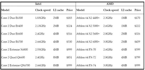
As a concrete example, consider the market for Central Processing Units (CPU), in which buyers (e.g. computer manufacturers) have needs for performance based on characteristics such as clock speed and cache memory. In addition, each of the two leading brands (Intel and AMD) has a comparative technological advantage at one of these two characteristics. In this context, buyers sort into di¤erent brands based on their particular needs: those who assign a higher value to clock speed are willing to pay a premium for Intel’s products, and the opposite is true for those consumers with a higher valuation for cache memory. It can be useful to summarize a the features of computer into a unitary measure of product quality. In this case, a consumer will naturally exhibit brand-speci…c tastes for quality. In fact, her willingness to pay for products of identical quality and di¤erent brand could not be represented by a …xed dollar amount. On the contrary, since brand preferences originate from di¤erences in product characteristics, this premium should be proportional to the quality of the goods being compared (a per-gigahertz premium, for the case of clock speed).

The results show that the equilibrium menus of contracts share the main qualitative fea-tures of the Mussa and Rosen (1978) monopoly allocation, namely e¢ cient quality provision for the highest type and quality distortions for all other types. One notable di¤erence is that …rms choose either to compete intensively for the entire market (providing strictly positive rents to all consumers) or to shut down the least pro…table segment of the market. The degree of correlation across buyers’brand preferences and the number of competing sellers have similar e¤ects on the equilibrium allocation: they increase market coverage, reduce quality distortions and increase the consumers’information rents.

In sharp contrast with other competitive screening models, our formulation of brand preferences implies that quality level o¤ered to the lowest consumer type is ine¢ ciently low. In consequence, compared to the existing papers, our model has the following implications in terms of observable variables: (i) a wider range of o¤ered quality levels, for a given distribution of consumers’tastes; and (ii) higher marginal prices for each quality level. We come back to the CPU market in section 7, and we use it as an example to illustrate these di¤erences and their implications for empirical work. Compared to our model, previous models would tend to overestimate the fraction of high valuation consumers, as well as the price sensitivity of their demand. Conversely, we …nd that our model would predict a much

higher demand sensitivity for low valuation consumers.

This paper is mainly related to the literature on competitive nonlinear pricing. Following the classi…cation in Stole (2007), early theoretical contributions with single dimensional models are given by Spulber (1989), Champsaur and Rochet (1989), and Stole (1995). In Ellison (2005), buyers di¤er both in taste for quality and in marginal utility of income. The more recent contributions of Armstrong and Vickers (2001), Rochet and Stole (2002), and Yang and Ye (2008) use multidimensional models to capture uncertainty both over brand preferences and taste for quality. In particular, the three latter papers assume that buyers’types have both a horizontal component (measuring brand preferences) and a vertical component (measuring taste for quality). We discuss these papers at length in section 7.

Our approach to brand preferences is also related to the theoretical and empirical discrete choice models of product di¤erentiation, such as those in Perlo¤ and Salop (1985), Anderson, De Palma, and Thisse (1992), and Berry, Levinsohn, and Pakes (1995). It is even more closely related to Berry and Pakes (2007), who develop a pure-characteristics demand model which removes the additive shocks and only de…nes consumers’ preferences over a set of product characteristics. Song (2007) adopts a pure-characteristics framework to estimate consumer demand and welfare in the CPU market. Nonlinear pricing with competition is also the object of a growing number of papers in empirical industrial organization. This strand of the literature includes the works of Miravete and Röller (2004) and Miravete (2009) on the cellular telephone industry, the paper by Busse and Rysman (2005) on the yellow pages industry, and the work of McManus (2007) on competing co¤ee chains.

2

The Model

Consider an imperfectly competitive market and let I = f1; : : : ; i; : : : Ig be the set of (identi-cal) sellers. Let there also be a continuum of buyers with unit demands. Buyers di¤er in their valuation of the quality of the goods produced by each …rm. A type for a buyer is a vector

of valuations = ( 1; :::; I) 2 RI: Buyer types are distributed on [ L; H]I according to

a distribution function F ( ) with a strictly positive and continuously di¤erentiable density f ( ).

The utility of a type buyer, consuming a good of quality qi, produced by …rm i and

sold at price pi is given by

v ( ; qi; pi) = iqi pi. (1)

We can view each type component i as the value of the match between consumer and the

an item of quality q produced by …rm i rather than by …rm j. In other words, consumers are willing to pay brand-speci…c premia that are proportional to product quality. It follows that demand for high quality products is less sensitive to absolute price reductions than demand for low quality items.

It can be useful to contrast (1) with the utility function commonly adopted in the

litera-ture on competitive screening. This literalitera-ture de…nes a buyer type as (t; x) = (t; x1; :::; xI)2

RI+1. The utility of type (t; x), when consuming a good of quality qi produced by …rm i and

sold at price pi is given by

v (t; x; qi; pi) = tqi pi+ xi. (2)

Suppose that both …rms i and j o¤er product q at price p: Under demand speci…cation (2),

a type (t; x) buyer is willing to pay xi xj more for …rm i’s item independently of the quality

level q. It follows that demand functions for high quality and high price items are more sensitive to equal percentage discounts than the corresponding demand functions for low quality items.

Our utility function formulation (1) can also be obtained from a more general model, in which preferences are de…ned over a vector of product characteristics, as in Berry and Pakes (2007). In this context, a brand is identi…ed by a combination of characteristics, while quality represents a scaling decision for products with similar combinations of characteristics. The rest of this paper works directly with the reduced form utility function (1), but we will come back to the product characteristics interpretation in section 6.

Each …rm i 2 I can produce goods of quality qi with the same technology c (qi), which

satis…es c (0) = 0, as well as c0_(q

i) > 0 and c00(qi) > 0 for all qi. If each …rm i chooses a

nonlinear tari¤ pi(qi), the indirect utility of a type consumer when purchasing from …rm

i is given by

Ui( ) = max

qi ( iqi pi(qi)).

Let U0( ) denote the consumer’s outside option and assume that U0( ) = 0 for all types :

A type consumer chooses to make her purchase from …rm i whenever this …rm provides

her the highest net utility,

Ui( ) Uj( ) for all j = 0; 1; :::; I.

Firm i’s market segment is de…ned as the set of types purchasing from i:

Zi =f 2 [ L; H]

I

: Ui( ) Uj( ) 8j 2 I[ f0gg.

i then seeks to maximize pro…ts: i = max qi;pi(qi) Z Zi [pi(qi( )) ci(qi( ))] f ( ) d .

3

Menu Pricing

As buyers have unit demands, we analyze competition among I sellers in an exclusive dealing framework. Throughout the paper, we maintain the assumption that …rms o¤er determin-istic menus of contracts. Under this assumption, it is without loss of generality to restrict attention to direct mechanisms. Furthermore, in these mechanisms, each …rm i only

condi-tions its price and quality o¤er on the buyer’s relevant type component i. The reason for

this result lies in the separability of the agent’s preferences. Under utility function (1), the agent’s ranking of items within each …rm’s menu is una¤ected by the menus o¤ered by other …rms. Therefore, following Martimort and Stole (2002), …rms cannot bene…t from o¤ering out of equilibrium contracts, i.e. price-quality pairs that are not chosen by any type in equi-librium. Restricting the message space to the type space then entails no loss of generality.

Furthermore, since all types = ( i; ) have the same preferences over the items in …rm i’s

menu, …rm i is unable to screen over all type components j 6= i. We can therefore restrict

attention to menu o¤ers in which the agent only reports type component i to each …rm i.

This feature of our model does not require any assumption on the distribution of types (e.g. independence). In fact, if type components were correlated, then each …rm i would

derive additional information about the buyer’s reservation utility from the revelation of i.

This information would certainly a¤ect the terms of the o¤er the …rm makes to each type i.

However, the …rm could not possibly use this information to further screen consumers, since

it lacks the instruments to discriminate among types with identical i and di¤erent i.

Therefore, each …rm’s optimal nonlinear pricing problem may be solved with the tradi-tional techniques of one-dimensional screening. In a direct mechanism, each …rm’s price and

quality o¤er is a function of the buyer’s reported type ^i: The utility of a type i buyer who

reports ^i when buying from …rm i may be written in the usual form:

Ui( i; ^i) = iqi(^i) pi(^i):

Normalize the buyers’ reservation utility to zero, and write the individual rationality con-straint as

Now de…ne each …rm’s utility provision schedule as

Ui( i) = max

^_i Ui( i; ^i):

The incentive compatibility constraints for the …rm’s problem are then given by the con-sumer’s …rst- and second-order conditions for truthful revelation of her type. By standard arguments, these are equivalent to:

U_i0( i) = qi( i), (4)

q_i0( i) 0. (5)

Consider a pro…le of incentive-compatible menus fqi( i) ; Ui( i)gIi=1. The incentive

com-patibility constraints (4) and (5) imply the indirect utility function Ui( i)is strictly

increas-ing. Therefore, a buyer of type chooses …rm i whenever her taste ifor brand i is su¢ ciently

large, relative her other type components _j6=i. We can then characterize the market share

of …rm i through a vector of I 1 threshold types j. Fixing a type component i, the

threshold _j represents the lowest taste for brand j that would induce consumer = ( i; )

to prefer …rm j over …rm i. The threshold types are de…ned as follows:

j(Ui( i) ; Uj) = 8 > < > : L if Ui( i) Uj( j) < 0 for all j, t s.t. Ui( i) = Uj(t) if t2 [ L; H], H if Ui( i) Uj( j) > 0 for all j. (6)

Notice that the set of types = ( i; ) that choose to purchase from …rm i depends on the

utility level U ( i) assigned to type i and on the entire utility schedules Uj( j) o¤ered by

…rms j 6= i. If we let fi( i) denote the marginal density of type component i, we can then

use equation (6) to de…ne …rm i’s market share function Mi(Ui( i) ; U i; i) as

Mi(Ui( i) ; U i; i) = Pr(Uj( j) Ui( i) 8j 6= i j i) fi( i)

= Pr( j j(Ui( i) ; Uj) 8j 6= i j i) fi( i). (7)

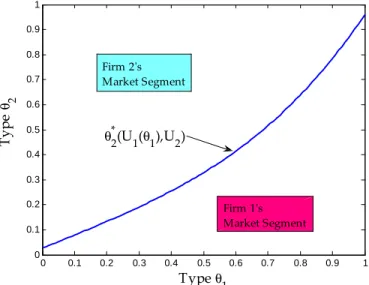
Figure 1 provides an illustration of the market segments in the case of a duopoly, when types are distributed on the unit square.

Figure 1: Threshold Types and Market Segments 0 0.1 0.2 0.3 0.4 0.5 0.6 0.7 0.8 0.9 1 0 0.1 0.2 0.3 0.4 0.5 0.6 0.7 0.8 0.9 1 Typeθ₁ Ty pe θ 2 Firm 1's Market Segment Firm 2's Market Segment θ₂*(U₁(θ₁),U₂)

Finally, de…ne the total surplus generated by providing quality qi to type i as

Si(qi; i) = iqi( i) ci(qi( i)).

Given the strategy pro…le fqj( j) ; Uj( j)g_j6=i of all …rms j 6= i, each seller i solves the

following problem: max qi( i);Ui( i) Z H L (Si(qi; i) Ui( i)) Mi(Ui( i) ; U i; i) d i (8) s.t. (3), (4), and (5).

The …rm’s objective function di¤ers substantially from the Mussa and Rosen (1978) monopoly problem. The di¤erences are mainly due to the e¤ect of buyers’brand-speci…c tastes on the competition among sellers. In particular, each …rm’s allocation of buyer types is endoge-nously determined, meaning that …rms can acquire larger market shares by o¤ering higher

utility levels. For a given strategy pro…le fqi( i) ; Ui( i)g

I

i=1, the utility levels o¤ered by

…rms j 6= i in‡uence the fraction of types ( i; ) served in equilibrium by …rm i. In other

words, market shares measure sales of products of quality qi( i)by …rm i. The market share

function Mi(Ui( i) ; U i; i) given in (7) may then be viewed as a weighted average of the

initial marginal distribution fi( i) that places a higher weight on high i types. Clearly,

4

Symmetric Equilibrium

We now present the necessary conditions for a symmetric equilibrium, and their implications for the properties of the solution. To simplify the notation, we now drop the subscript i

from the …rms’strategies, and (with a slight abuse of notation) we let type components i

be identically and independently distributed according to a univariate distribution F ( i).

We extend the analysis to the case of correlation in section 6.

The necessary conditions for a symmetric equilibrium can be expressed as a second-order

di¤erential equation in U ( i). For greater clarity, Proposition 1 presents them in terms of

both functions q ( i) and U ( i), which are linked by incentive compatibility constraint (4),

or equivalently by condition (10) in what follows. Proposition 1 (Necessary Conditions)

The necessary …rst-order conditions for quality and utility provision at a di¤erentiable sym-metric equilibrium are given by:

c00(q ( i)) q0( i) = 2+ c (q ( i)) + U ( i) q ( i) c0(q ( i)) (I 1) f ( i) F ( i) +( i c0(q ( i))) f0₍ i) f ( i) , (9) where U ( i) = U ( L) + Z i L q (t) dt, (10)

with the boundary condition

c0(q ( H)) = H: (11)

The transversality condition (11) delivers the well-known “no distortion at the top”result. In the Mussa and Rosen (1978) monopolistic price discrimination model, the …rm extracts all the rent from the lowest type in the distribution. The equilibrium nonlinear tari¤ may

therefore be found using the boundary conditions (11) and U ( L) = 0.

In a competitive environment, this second boundary condition is no longer valid, because information rents have a positive impact on market shares and may therefore increase pro…ts.

In particular, as shown in condition (10), the utility of the lowest type U ( L) shifts the

entire rent function U ( i). As such, it represents a free endpoint for the …rm’s problem.

This immediately allows us to conclude that the shadow value of the incentive compatibility

constraint (4) must be zero at L. In the Rochet and Stole (2002) model, in the absence of

bunching, this condition delivers the “no distortion at the bottom” result.3

3_{This feature is also present in other contexts where the objective function is not everywhere decreasing} in information rents. For instance, see the optimal taxation model of Seade (1977).

This is not the case in our model, where the di¤erential equation (9) has a singularity

at L. This occurs because …rm i’s market share of types i = L is equal to zero, since the

probability of another type component _j6=i being larger than Lis equal to one. As we show

in the Appendix, this implies that shadow value of the incentive compatibility constraint (4)

is equal to zero independently of the level of qL. Therefore, e¢ cient quality provision at the

bottom of the distribution is not an equilibrium feature in the brand-speci…c tastes model. Indeed, as we show in Proposition 2, the quality level served to the lowest type in equi-librium must be distorted downwards from the e¢ cient level. This feature of the equiequi-librium brings the monopoly and oligopoly results closer together, and represents the key novel im-plication of the brand-speci…c tastes model. We stress that this feature of our model extends

to the case of correlation across type components, as long as Pr ( j > Lj i = L) = 1 for

all i and j.

Proposition 2 (Lowest Type)

1. If the market is covered in equilibrium, the utility level of the lowest type is given by

U ( L) = c0(q ( L)) q ( L) c (q ( L)) . (12)

2. The quality level provided to the lowest type is distorted downward ( L > c0(q ( L))).

An implication of Proposition 2 is that a symmetric equilibrium cannot involve both positive quality provision and full surplus extraction at the bottom of the distribution. To gain some intuition about this result, observe that the provision of positive quality levels to

any type i requires the …rms to incur in the shadow cost of the incentive constraints for

all higher types. Not providing a type with a strictly positive utility level e¤ectively means making zero sales. Therefore, o¤ering positive quality and zero utility (as in the monopoly case) bears only costs and no bene…ts to the …rm.

Perhaps more importantly, condition (12) in Proposition 2 allows us to rule out e¢ cient

quality provision at the bottom ( L = c0(qL)). If that were the case, direct substitution into

(12) would immediately imply that …rms leave the entire surplus S (q ( L) ; L) to the buyer,

thereby obtaining zero pro…t margins on the lowest type.4 _{Per se, this is not su¢ cient to}

rule out e¢ ciency at the bottom, because each …rm i never actually serves any consumer

with i = L. Furthermore, we know from condition (10) that U ( L) is chosen optimally,

taking into account its e¤ect on the entire rent function U ( i), and that competition is

…ercer for the lower types, which are more price-elastic. Therefore, it is not a priori clear that lowering the utility of the lowest type (i:e: shifting the rent function down) can increase

the …rm’s pro…ts. However, as we show in the Appendix, e¢ cient quality provision at the

bottom would imply that pro…t margins on types i in a neighborhood of L vanish faster

than …rm i’s equilibrium market share. Intuitively, the …rm can then pro…tably raise prices

(at the expense of market shares) and obtain positive pro…ts in a neighborhood of L.

The positive distortions result brings our model closer to the …ndings of Yang and Ye (2008). The main di¤erence with this paper is that Yang and Ye (2008) assume vertical types

t are uniformly distributed on [0; 1] : As a result, a set of lowest types are inevitably shut

down, because they provide a cost in terms of incentives, and no surplus. Quality distortions are then a consequence of shut down. In other words, the main novel element of our …ndings is that quality distortions arise even under full market coverage.

In addition to these economic insights, Proposition 2 allows us to use (12) as boundary condition, together with (11), to solve for the symmetric equilibrium under the hypothesis of

full market coverage. In the alternative case, in which all types i below a lower threshold 0

are excluded in equilibrium, we can use (11) together with boundary conditions U ( 0) = 0

and q ( 0) = 0, in order to solve (9).

In the Appendix, we provide two di¤erent algorithms to compute the solution in the

cases of full and partial market coverage, respectively.5 These algorithms include a simple

procedure, based on a result by Seierstad and Sydsaeter (1977), to verify the su¢ ciency of our system (9)-(11). There are two main di¢ culties associated with analytically checking these conditions: the …rst one arises because a closed form solution to the …rst-order conditions can only be obtained in a few special cases; the second one originates from the equilibrium functional form of market shares, which (when all …rms j 6= i adopt the same strategy) is

given by FI 1₍

j(Ui( i) ; Uj)). This makes it di¢ cult to show the concavity of the objective

function in the information rents. The Appendix contains a duopoly example, with uniformly distributed types and quadratic costs, which admits a closed-form solution and for which we verify the second order conditions analytically. Both for this reason, and for tractability, we now specialize the model by introducing these two assumptions.

5

Uniform-Quadratic Model

Throughout this section, we maintain the following assumptions:

c (qi) = 1 2q 2 i; (13) F ( i) = i L H L i.i.d. 8i. (14) These restrictions allow us to clearly separate our results with those of Armstrong and Vickers (2001) and Rochet and Stole (2002), and to provide some insights into the comparative statics of the equilibrium nonlinear prices with respect to the number of competing …rms.

Assessing the e¤ects of competition requires some attention. First, because our model lacks a general existence and uniqueness result, we need to rely on numerical solutions to ensure that the comparative statics exercise is well-founded. Second, increasing the number of …rms enhances competition, but also multiplies the preference space of the consumer and the potential social surplus. This e¤ect is similar to what happens in discrete choice models, where consumers have preferences over product characteristics. In that context, the e¤ect of introducing a new product depends on the degree of similarity with the existing ones. In section 6, we relate the degree of similarity of the underlying product characteristics to the correlation among brand-speci…c taste parameters. In the case of positive correlation, the e¤ects of enlarging the preference space are then clearly dampened. Indeed, the e¤ects of introducing new brands are most stark in the independent types case. As such, the analysis under the independence assumption provides a benchmark, and a lower bound, on the competitive e¤ects of increasing the number of …rms.

The e¤ect of a higher number of competitors need not a priori dominate the stochastic

im-provement in the distribution of consumers’valuations.6 _{Therefore, in the uniform-quadratic}

model, we vary the number of products I, and we contrast the case of competition with the multiproduct monopolist’s solution. The following results assume (and numerically validate this assumption) that there is a unique solution to the …rst order conditions, and that the second order conditions are satis…ed. In particular, Proposition 3 compares the e¤ect of an increase in the number of brands I in the cases of competition and multiproduct monopoly. In order to facilitate this comparison of the equilibrium menus, we solve the monopolist’s problem under the assumptions of anonymous pricing. This corresponds to forcing the mo-nopolist to literally posting I menus of contracts. Formally, this means we restrict the direct mechanisms o¤ered by the monopolist to o¤er the same set of price-quality options to all 6_{The work of Chen and Riordan (2008) addresses exactly this point in the context of a duopoly model} with price competition.

buyers, regardless of their reported types. Proposition 3 (Comparative Statics)

Assume (9)-(11) admit a unique solution, which is in fact an equilibrium. 1. In the competitive model, as the number of …rms I increases:

(a) market coverage (weakly) increases;

(b) utility provision (weakly) increases for all buyer types; (c) quality provision (weakly) increases for all buyer types.

2. In the monopoly model, as the number of products I increases, the quality and utility

levels qi( i) and Ui( i) decrease for all i.

Consider …rst the multiproduct monopolist’s problem. Since consumers have unit de-mand, restricting attention to anonymous pricing schemes reduces the monopolist’s problem to one of one-dimensional screening. Each product i’s market share of consumers is given

by Mi = f : i = maxj2I( j)g. In other words, each product i is sold as if the monopolist

were facing a population of consumers distributed according to FI₍

i). Therefore the quality

schedules are given by

qm_i ( i; I) = i 1 FI₍ i) IFI 1₍ i) f ( i) .

Proposition 3 shows that the number of products yields an increase in the magnitude of the quality distortions. In terms of indirect utility, buyers may either gain or lose. In particular, each consumer draws a taste parameter for the new product. If this new type component is not high enough, her utility will decrease. Similarly, the e¤ect on overall market coverage is ambiguous, as each individual product sells to fewer buyer types, but new products capture a share of the market as well.

The reasons for the di¤erent comparative statics results in the competitive and monopoly models lie in the opportunity cost of providing utility. In the monopoly case, there are no gains in terms of market shares. An increase in the number of products only enlarges the preference space. This creates the possibility for the …rm to exploit the gains from additional product variety. In the competitive case, an increase in the number of …rms I a¤ects both the size and the composition of each …rm’s equilibrium market shares. The size of the overall market shares obviously decreases, reducing both the costs and the bene…ts of providing extra utility in a similar fashion. However, an increase in competition also increases the proportion

consumers with a higher iserved by each …rm. This means that the provision of utility at the

top of the distribution is now more rewarding. As a consequence, the incentive compatibility

requirements of distorting quality for low i types are less stringent, resulting in higher utility

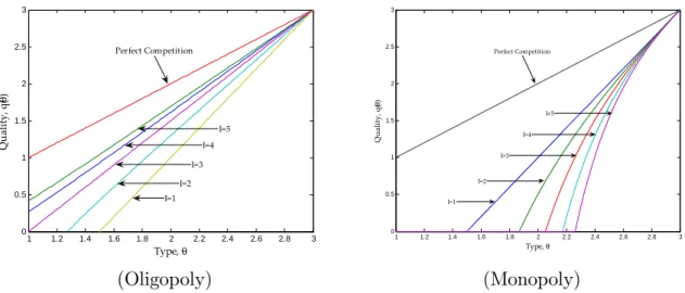
e¢ cient levels and the agents’ rents increase. Qualities remain distorted downward at the bottom of the distribution, but the range of quality levels o¤ered in equilibrium decreases.

In Figure 2, we show the equilibrium quality levels when i 2 [1; 3] for the case of

competition (left panel) and multiproduct monopoly (right panel).

The forces underlying the comparative statics results in our model di¤er sharply from

those in other models of nonlinear pricing with spatial competition.7 These models adopt a

linear-city or circular-city framework. As a consequence, …rms directly compete only with their “neighbors.” By allowing a more general formulation of brand preferences, our model allows for “global” competition among several …rms, as is the case in the applied discrete-choice literature. The extent to which two rival …rms are competing is then determined by the speci…c distribution of consumers’brand preferences.

Figure 2: Equilibrium Quality Supply, Uniform Distribution

1 1.2 1.4 1.6 1.8 2 2.2 2.4 2.6 2.8 3 0 0.5 1 1.5 2 2.5 3 Type,θ Q ual ity, q( θ ) Perfect Competition I=5 I=4 I=3 I=2 I=1 (Oligopoly) 1 1.2 1.4 1.6 1.8 2 2.2 2.4 2.6 2.8 3 0 0.5 1 1.5 2 2.5 3 Q ual ity, q( θ ) Type,θ Perfect Competition I=2 I=4 I=5 I=3 I=1 (Monopoly)

Finally, we point out that in the uniform quadratic model, the entire market is served,

and the lowest type i = L receives exactly zero quality when the following relationship is

satis…ed:

H =

3 + I

2 L:

As we show in the Appendix, in this case the system of …rst-order conditions for a symmetric equilibrium has an analytic solution characterized by linear quality provision:

q ( i) =

(I + 3) i 2 H

I + 1 .

For example, in Figure 2 (left), the analytic solution is obtained for I = 3, H = 3, L= 1.

The following corollary can then be derived from Proposition 3. 7_{For example, Spulber (1989), Stole (1995), and Yang and Ye (2008).}

Corollary 1 (Market Coverage)

Assume (9)-(11) admit a unique solution, which is in fact an equilibrium. Then the market

is fully covered if and only if I 2 ( H= L) 3.

An equivalent interpretation of this result suggests that whenever the ratio of L to H

exceeds a critical value the equilibrium involves the provision of strictly positive utility to all

types. Conversely, whenever the ratio of Lto H falls short of the critical value, (3=2 + I=2),

the equilibrium involves the shutdown of the lowest types. For the case of a duopoly, the threshold is equal to 2=5, which for example is lower than the threshold of 1=2 obtained in the Mussa and Rosen (1978) monopoly model.

6

Correlated Types and Product Characteristics

Correlation across brand preferences directly a¤ects the intensity of competition by in‡uenc-ing the distribution of buyers’outside options. In particular, positive and negative correlation

may be expected to respectively increase and relax competition between …rms.8

In this section, we derive the necessary conditions for a symmetric equilibrium. These conditions generalize those in Proposition 1. They also serve as a building block for the analysis of the link between product characteristics and brand preferences. We show that brands selling products with similar characteristics generate positively correlated tastes for quality, and provide an illustration of this link through an example with a bivariate normal type distribution.

6.1

Symmetric Equilibrium Conditions

Assume that types is distributed over [ L; H]I according to a symmetric distribution F ( )

with density f ( ). Analogously to the independence case, …x a pro…le fqi( i) ; Ui( i)gI_i=1 of

incentive-compatible menus and a seller i. The indi¤erent types _j(Ui( i) ; Uj) are de…ned

as in (6). Firm i’s market share of participating types ( i; ) may be written as

Mi(Ui( i) ; U i; i) =

Z _j(Ui( i);Uj) L

f ( ) d i.

As noted in section 3, the distribution of types does not a¤ect the buyer’s ranking of the items within each …rm’s menu. The …rms’incentive compatibility and individual rationality 8_{The case of perfect negative correlation has been analyzed by Spulber (1989), who …nds that …rms operate} in a local monopolies regime. The case of perfect positive correlation has been analyzed by Champsaur and Rochet (1989), who introduce vertical di¤erentiation by letting …rms choose quality ranges …rst, and then compete in nonlinear prices.

constraints are therefore unchanged and …rm i’s objective function may be formulated as follows: max qi( i);Ui( i) Z H L Z j(Ui( i);Uj) L (Si(qi; i) Ui( i)) f ( i; i) d id i.

The …rst order conditions for a symmetric equilibrium are then stated in the following

propo-sition. Let ( i) denote the multiplier on the incentive compatibility constraint (4) for each

…rm i.

Proposition 4 (Necessary Conditions with Correlation)

The necessary …rst-order conditions for quality and utility provision at a di¤erentiable sym-metric equilibrium are given by:

( i c0(q ( i))) Z i L f ( ) d i+ ( i) = 0, (15) Z i L f ( ) d i Si(qi; i) U ( i) q ( i) X j6=i Z i L :: Z i L f ( )d i j = 0( i) , (16) H c0(q ( H)) = 0: (17)

In the Appendix, we provide a duopoly example based on the Farlie-Gumbel-Morgenstern copula (see Nelsen (2006) for more details), in which the degree of correlation is small. We show that the qualitative properties of the equilibrium under independence carry over to the case of correlation. One drawback of using the FMG copula is that it only allows for low values of correlation. We consider higher degrees of correlation in the next example. Before we do so, we demonstrate how brand-speci…c tastes for quality may be derived from a pure characteristics demand model. We then apply the equilibrium conditions from this subsection to this new “micro-founded” model.

6.2

Product Characteristics

Consider a hedonic oligopoly model in which products are de…ned as bundles of

charac-teristics x 2 RK _{with K 2: Let}

k be the consumer’s marginal utility of consuming

characteristic k: The utility of a buyer consuming product x = (x1; :::; xK)is then given by:

u ( ; x) = K X

k=1

kxk p (x).

This speci…cation is virtually identical to the one adopted in the pure characteristics demand model of Berry and Pakes (2007). In contrast with the earlier discrete-choice

em-pirical literature, which takes all product characteristics as given, we assume that each …rm can produce several di¤erent quality levels of its variant of the product. We de…ne …rm i’s

variant of the product as a bundle of characteristics i = ( i1; :::; iK). In other words, …rm

i’s production possibility set is given by the i ray in RK.

Yi = x2 RK : x = (q i1; :::; q iK) ; q 2 R+ .

Production costs are expressed in terms of quality levels q only. This formulation allows one to identify a brand with an exogenously determined variant of the product, and quality with an endogenously chosen scaling parameter that distinguishes products of the same brand.

The utility of a consumer with preferences is then given by

u ( ; i; q) = q

K X

k=1

k ik p (q) :

We can now de…ne

i( ) =

K X k=1

ik k

and obtain the original formulation of brand-speci…c tastes for quality (1) from preferences

over product characteristics. The degree of heterogeneity between …rms’ variants i is an

index of product di¤erentiation and, as such, measures the intensity of competition in the market. When adopting the original formulation (1), given an initial distribution of buyers’ tastes for characteristics, the degree of similarity between …rms’variants is directly related to the degree of correlation between brand-speci…c taste parameters in the population. In order to obtain a tractable model with a symmetric equilibrium, we only need to ensure

that all type components i are distributed over the same support. This can be achieved

by assuming that P_k ik = a for all i and that the distribution of each component k

has the same support. To summarize, the brand-speci…c model represents a concise way of summarizing tastes for characteristics into a single dimensional brand-speci…c index. We now illustrate an example based on the multivariate normal distribution.

6.3

The Multivariate Normal Case

Let tastes for each characteristic k be identically and independently distributed according to the following normal density:

k N ;

De…ne …rm i’s variant of the product by i = ( i1; i2). The two …rms’production possibility sets are then given by:

Xi = x2 R2 : x = (q i1; q i2) ; q 2 R+ , 8i = 1; 2:

Brand-speci…c tastes can therefore be de…ned as:

i( ) = i1 1+ i2 2:

Under the normal distribution assumption for k, the brand speci…c tastes ( 1; 2)are jointly

normally distributed with mean vector

m = (( 11+ 12) ; ( 21+ 22) ),

and dispersion matrix

= " v1 pv1v2 p_v 1v2 v2 # , where vi = 2(( i1) 2 + ( i2) 2

)denotes the variance of each type component. The correlation

coe¢ cient is given by = 1 2

k 1kk 2k = cos (t), where t denotes the angle between the two

char-acteristics vectors ( 11; 12)and ( 21; 22). Therefore, in this model, the degree of similarity

between the two …rms’variants of the product determines the correlation coe¢ cient between the consumers’tastes, and hence the intensity of competition on the market. For example, if …rms characteristics are collinear, the brand-speci…c tastes are perfectly correlated, and Bertrand equilibria are obtained. If characteristics are orthogonal, types are independent, and the analysis is identical to that of section 4.

To apply these …ndings, consider an example in which types i follow a symmetric

bi-variate normal distribution. In particular, we make the following assumptions on consumers’

preferences ( ) and …rms’variants ( i):

k N (0; 1) 8k = 1; 2

2 X

k=1

( ik)2 = 1 8i = 1; 2.

In other words, we let each taste parameter _k be distributed according to a standard

normal, and we assume that variants of the product lie on the unit radius circle. Under

mean vector m = (0; 0) and dispersion matrix = " 1 1 # , where = 1 2 k 1kk 2k.

We now use the symmetric equilibrium conditions derived above to characterize the solution of this model for di¤erent values of . In order to compute a numerical solution, we need to truncate the distribution of each type component at a common upper bound

( H). It may be easily shown that the truncation point only a¤ects the terminal conditions

and not the di¤erential equations governing the solution. The probability density function is then given by f ( 1; 2) = 1 2 p1 2exp 2 1 2 1 2+ 22 2 (1 2₎ ,

which means that the market share function may be expressed in closed form via the error

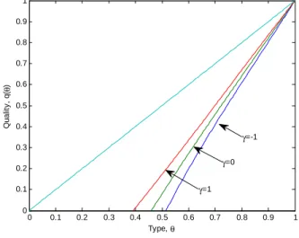
function erf ( i). In Figure 3, we let costs be quadratic, and let the correlation parameter

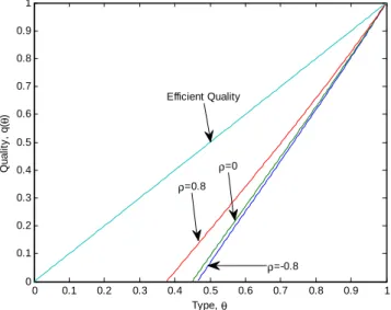
take values in the set f 0:8; 0; 0:8g.

Figure 3: Duopoly Quality Provision - Bivariate Normal

0 0.1 0.2 0.3 0.4 0.5 0.6 0.7 0.8 0.9 1 0 0.1 0.2 0.3 0.4 0.5 0.6 0.7 0.8 0.9 1 Type,_θ Qual it y , q( θ ) Efficient Quality ρ=0.8 ρ=0 ρ=-0.8

The numerical results con…rm the intuition that positive correlation across type components increases the e¢ ciency of the quality supply schedules. Quite surprisingly, even values of the correlation coe¢ cient as high as 0:8 do not dramatically improve the e¢ ciency of the allocation. In the opposite case of negative correlation, low types’outside options are higher, and for some parameter values the equilibrium quality provision lies below the monopoly level.

7

Comparison with the Literature

The papers most closely related to the present work are those by Armstrong and Vickers (2001), Rochet and Stole (2002), and Yang and Ye (2008). As alluded to previously, in these papers buyers value quality uniformly, and their brand preferences are given by seller-speci…c additive utility shocks (see utility function formulation (2)). These shocks are assumed to be uncorrelated with the quality of the purchased product, and distributed independently from the tastes for quality in the population. Thus, these models separate the consumer’s “vertical”preferences over veri…able product quality from her “horizontal”brand preferences. However, as a result, the relative value of purchasing products of similar quality from di¤erent …rms is independent of the quality of the chosen products. We now illustrate the di¤erent the theoretical results of these papers and our model. We then turn to their empirical predictions and discuss the implications of taking each model to the data, in the context of the CPU market example.

7.1

Model Predictions

The main apparent di¤erence between our results and those of Rochet and Stole (2002) lies in the equilibrium quality schedules. When the market is covered, Armstrong and Vickers (2001) and Rochet and Stole (2002) predict the e¢ cient quality levels are produced in

equi-librium. When not all types (tL; ) participate, the Rochet and Stole (2002) allocation is

characterized by e¢ ciency at the top and at bottom. This is in contrast with our result in

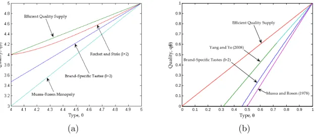
Proposition 2, which predicts quality distortions for all types, including L. Figure 4, panel

(a), considers an example where types i (and vertical types t) are distributed uniformly on

[4; 5]. It shows that our model predicts more severe quality distortions for all types.

This di¤erence is due to the equilibrium composition of market shares, and to their sensitivity to prices in the two models. To clarify this point, remember that in the Armstrong and Vickers (2001) and Rochet and Stole (2002) models, at a symmetric equilibrium with full market coverage, each …rm serves a constant fraction of all vertical types t. In equilibrium, each …rm e¤ectively serves a population of consumers whose types are distributed according to (1=I) f (t). Conversely, in the symmetric equilibrium of our model, types in the market

segment of …rm i are distributed according to FI 1₍

i) f ( i), which indicates a relatively

larger presence of high types.

To obtain a meaningful comparison between the di¤erent models, we appropriately mod-ify the initial distributions of types. In particular, consider the model in Yang and Ye (2008), which extends the one in Rochet and Stole (2002) to the case of imperfect market coverage. Vertical types t in the model of Yang and Ye (2008) are uniformly distributed on [0; 1]. For

Figure 4: Equilibrium Quality Provision - Comparison (a) 0 0.1 0.2 0.3 0.4 0.5 0.6 0.7 0.8 0.9 1 0 0.1 0.2 0.3 0.4 0.5 0.6 0.7 0.8 0.9 1 Type,θ Q ual ity, q( θ )

Efficient Quality Supply

Yang and Ye (2008)

Mussa and Rosen (1978) Brand-Specific Tastes (I=2)

(b)

all types t, market shares are de…ned by x (Ui(t) ; Uj(t)), which is the solution to:

Ui(t) x = Uj(t) (1 x ) :

At a symmetric equilibrium, over the full coverage region, market shares are equal to one-half. Furthermore, the sensitivity of market shares to utility provision is constant and equal to

@x (Ui(t) ; Uj(t))

@Ui(t)

= 1

2 8t.

In our model, let type components i be distributed according to F ( i) =

p

i on [0; 1].

As in the model of Yang and Ye (2008), the equilibrium market share of each …rm is given

by F ( i) f ( i) = 1=2: However, in the present work, market shares are determined by the

solution to Uj( j) = Ui: Therefore, their sensitivity to utility provision is given by

@ _j(Ui( i) ; Uj) @Ui = 1 U0 j( j) = 1 qj(Ui( i) ; Uj) :

Since quality is an increasing function of type, utility provision has a positive but declining e¤ect on market shares. In other words, the value to …rm i of providing additional utility to high-valuation types is much lower than in Yang and Ye (2008), because those types require larger discounts in order to switch brands. Figure 4, panel (b), compares our equilibrium allocation with the model in Yang and Ye (2008), holding constant the composition of the equilibrium market shares. Distortions are greater in the present work, despite the stochas-tically dominated initial distribution of types. We can then conclude that di¤erences in the

sensitivity of market shares drive the main qualitative di¤erences between the two classes of models.

7.2

Implications for Observable Variables

The most immediate implication of quality distortions in terms of observable variables con-cerns the variety of products o¤ered by each …rm. In particular, when the market is covered and there is no bunching, our model predicts a wider range of product qualities than the

previous models. Quite simply, the upper bound on quality is identical ( H = c0(qH)), while

the lowest o¤ered quality is below the e¢ cient level for the lowest type ( L > c0(qL)).

A more subtle implication of quality distortions is related to the actual nonlinear prices

pi(qi). Under our linear utility speci…cation, the marginal price charged for each quality

level is equal to the type of the consumer buying that product. This is most clearly seen from the …rst order condition for type ’s choice from …rm i’s menu,

i = p0i(qi) : (18)

More severe quality distortions imply that a given quality level is assigned to a higher-valuation buyer, and hence it is sold at a higher marginal price. To illustrate the di¤erence with the Rochet and Stole (2002) model, Figure 5 shows the equilibrium marginal prices,

when types i (and vertical types t) are distributed uniformly on [4; 5].

Figure 5: Equilibrium Marginal Prices - Comparison

3.5 4 4.5 5 4 4.1 4.2 4.3 4.4 4.5 4.6 4.7 4.8 4.9 5 Quality, q M arg ina l P rices , d p(q )/d q

Rochet and Stole Brand-Specific Tastes

7.3

Inference from Data

In the Rochet and Stole (2002) and in our model, the econometrician can use price and quality data, together with the …rst-order condition for the consumer’s problem (18) to make inference about the valuations of the consumers buying each product. For example, if the utility function is assumed to be known, the highest and lowest marginal prices identify

H and L.

In addition, if data on production costs is available, the presence of quality distortions at the top and at the bottom of the menu can be tested directly. This is the case, for example, of McManus (2007), who studies specialty co¤ee chains, and …nds no distortions at the top of the menu (large, sweet espresso drinks), and positive distortions in the size of all other co¤ee products. He interprets the diminishing distortions towards the bottom as evidence of more intense competition for these items. The results of McManus (2007) are in line with the …ndings of Proposition 2, as well as with the our model’s feature of more price-sensitive demand for buyers of low-quality items.

In the absence of information on cost, but with knowledge of each product’s market share, the existing models and the present work can yield very di¤erent estimates of the distribution of valuations and of demand elasticity. We illustrate these di¤erences in the context of our motivating example of the CPU market. In this market, the relevant product characteristics are clock speed and cache memory. Table 1 summarizes these features for the main Intel and AMD processors for sale in 2007. Consistent with our approach in section 6.2, AMD processors generally run faster than their Intel counterparts, but have a smaller cache memory.

A competitive nonlinear pricing model may be employed to analyze the two …rms’choices of product characteristics and prices simultaneously. In particular, the present model would construct a separate quality measure for each brand, by considering di¤erent linear combi-nations of clock speed and cache memory. Conversely, the existing models are based on a one dimensional vertical type. Thus, they would de…ne quality as a linear combination of

the two characteristics which is common to both brands.9

In both models, the observed market shares provide information on the underlying dis-tribution of consumers’valuations for each product. The main di¤erence in this respect is that the Rochet and Stole (2002) model would attribute each purchase of a high quality product to a “high t” type, and explain the choice of brand entirely through consumer-…rm …xed e¤ects (equivalently, the logit errors). Conversely, our model would recognize that con-sumers sort based on their idiosyncratic needs, and hence that the observed market shares

correspond to a selected sample of consumers.10 _{In other words, some high-quality purchases}

should be attributed to consumers with a particularly high taste for one brand, but not for the other. Therefore, our model would yield much lower estimates of the number of con-sumers with uniformly high valuations. This is a general feature of empirical applications of discrete choice models, but in particular of Song (2007), who considers a one-dimensional pure characteristics approach, and of Hendel (1999), who matches buyer characteristics with product characteristics in a multinomial logit model.

Finally, in order to explain the observed marginal prices, the Rochet and Stole (2002) model would estimate a single transportation cost parameter for all vertical types t. Instead in the present model, the degree of horizontal di¤erentiation is implicit in the distribution of brand preferences. As shown in section 6.2, this distribution summarizes the buyers’tastes for characteristics and the properties of each brand’s products. Compared to the Rochet and Stole (2002) results, the implied sensitivity of demand will be much lower at the top of the type distribution. For example, if a consumer of the top Intel product (QX6700) were to switch to AMD, she would most likely choose the FX-72 or FX-74, which have considerably di¤erent characteristics (most notably, half as much cache memory). Even though these

products might have very similar quality levels qIN T EL and qAM D, this buyer requires a very

large discount in order to consider switching brands. Conversely, market share sensitivity is higher towards the bottom, where absolute di¤erences in product characteristics are smaller. 9_{This might already be a problem, as there exists no linear combination of clock speed and L2 cache that} yields increasing price functions for both brands in Table 1.

10_{Loosely speaking, many di¤erent applications bene…t from a large cache memory, while a single, simpler} application bene…ts from a higher clock speed.

8

Conclusion

This paper develops a competitive nonlinear pricing model, where the buyers’valuation of quality depends on the product’s brand. In particular, buyers of high quality items are willing to pay larger brand premia, leading to a lower price elasticity for high quality items. In the symmetric equilibrium, brand-speci…c tastes for quality restore the quality distortions that may be absent from earlier random participation models, and rule out the possibility of marginal cost pricing.

However, our model does not nest those of Armstrong and Vickers (2001), Rochet and Stole (2002) and Yang and Ye (2008), and is to be considered a complement rather than substitute to their approach. Another contribution of this paper is to build a tighter con-nection between the empirical and theoretical literature on di¤erentiated products oligopoly. In particular, it relates the pure characteristics demand model of Berry and Pakes (2007) to a competitive nonlinear pricing problem. Under particular functional forms, the resulting screening model with correlated types may be solved for a symmetric equilibrium. This al-lows us to trace out the implications of consumers’preferences over multidimensional product characteristics, when …rms simultaneously choose prices and qualities.

A natural extension of our model considers a dynamic game in which product charac-teristics are determined in a …rst stage and competitive price discrimination (e.g. through two-part tari¤s) takes place in the second stage. Another, more ambitious extension con-sists of integrating proportional and additive brand preference components in the consumer’s choice problem. At present, these extensions constitute the object of further research, but both represent important steps towards adopting the present model for empirical work.

Appendix

Proof of Proposition 1: _{Suppose all …rms j 6= i are o¤ering an identical menu of contracts}

(qj( j) ; Uj( j)). The Hamiltonian for …rm i may be written as

H (qi; Ui; i; i) = ( iqi c (qi) Ui) FI 1( j(Ui( i) ; Uj))f ( i) + iqi. (19)

The …rst order conditions for (19) with respect to quality and utility provision are given by:

( i c0(qi)) FI 1( j (Ui( i) ; Uj))f ( i) + i = 0 (20) iqi c (qi) Ui qj(Ui( i) ; Uj) (I 1) FI 2( _j(Ui( i) ; Uj))f2( i) (21) +FI 1( _j (Ui( i) ; Uj))f ( i) = 0i( i) i( H) = 0. (22)

At a symmetric equilibrium, qj( j) = qi( i) and j = i: Di¤erentiating (20) with respect

to i, solving for 0i( i), and substituting into (21) delivers the expressions for …rst order

conditions (9)-(11).

Proof of Proposition 2: (1.) Consider the necessary conditions (9)-(11) and drop the

argument ( i). Rearranging condition (9) one obtains:

U ( i) = c0(q ( i)) q ( i) c (q ( i)) 2 c00_{(q (} i)) q0( i) I 1 F ( i) f ( i) q ( i) (23) i c0(q ( i)) I 1 F ( i) f0( i) f2₍ i) q ( i),

which holds for all i > L. Since both F and f are assumed to be continuously di¤erentiable,

and f > 0 for all i, by the continuity of U , we have

lim i! L F ( i) f ( i) = lim i! L F ( i) f0( i) f2₍ i) = 0.

Therefore, taking the limit of the right hand side of expression (23) as i ! L, we can

conclude that:

U ( L) = c0(q ( L)) q ( L) c (q ( L)),

(2.) No …rm o¤ers qualities in excess of the socially e¢ cient level, as it could o¤er the same utility levels at a lower cost by reducing quality. Therefore, we seek to rule out the following allocation:

c0(q ( i)) < i 8 i 2 ( L; H),

c0(q ( L)) = L,

c0(q ( H)) = H.

De…ne the pro…t margin on type i as

( i), iq ( i) c (q ( i)) U ( i) :

Suppose towards a contradiction that c0_{(q (}

L)) = L.Condition (12) immediately implies

( L) = 0. Di¤erentiating and using the incentive compatibility constraint (4), we obtain

0₍

L) = ( L c0(q ( L))) q0( L) + q ( L) U0( L) = 0. (24)

At a symmetric equilibrium, …rst order condition (21) may be written as

FI 1( i) f ( i)

( i) q ( i)

(I 1) FI 2( i) f2( i) = 0( i) : (25)

Both q ( i)and f ( i)are strictly positive. Therefore, as i ! L, condition (24) implies that

the second term in (25) goes to zero at rate (d i)I. Conversely, the …rst term goes to zero

at rate (d i)I 1. Consequently, there exists an " > 0 such that

Z L+" L

0₍

i) d i = ( L+ ") ( L) = ( L+ ") > 0,

since …rst order condition (20) implies ( L) = 0: But then …rst order condition (20) also

implies the …rm is o¤ering quality c0(q ( L+ ")) > L+ ", which is in excess of the e¢ cient

level and clearly sub-optimal.

We now use restriction (12) from Proposition 2 to implement two algorithms to compute the symmetric equilibrium.

Computing the solution under full market coverage: First, choose an initial value

q0 for q ( L) on [ L; H]. Then solve the system using c0(q ( H)) = H and q ( L) = q0 as

boundary conditions, and verify whether condition (12) holds. If it does, then the equilibrium

step. This procedure must be repeated until the right-hand side of (12) converges to the

corresponding U ( L; q0). The limit q0, along with the associated schedules q ( i)and U ( i),

result in the computed equilibrium. To verify that the second order conditions are satis…ed,

use …rst order condition (20) to compute the equilibrium value of ( i). Then check that the

computed q ( i) and U ( i) maximize the modi…ed Lagrangean of Seierstad and Sydsaeter

(1977):

L (qi; Ui; i) = ( iqi c (qi) Ui) FI 1( j (Ui( i) ; Uj))f ( i) + ( i) qi+ 0( i) Ui. (26)

Computing the solution under partial market coverage: First, choose an initial value

for 0 on [ L; H]. Then solve the system using c0(q ( H)) = H and U ( 0) = 0 as boundary

conditions and verify whether the condition q ( 0) = 0 holds or not. If it does, then the

equilibrium has the desired properties; otherwise, adjust the initial value for 0 and go back

to the …rst step. This procedure must be repeated until q ( 0) converges to zero. The limit

0, along with the associated schedules q ( i)and U ( i), result in the computed equilibrium.

To verify that the second order conditions are satis…ed, use …rst order condition (20) to

compute the equilibrium value of ( i). Then check that the computed q ( i) and U ( i)

maximize the modi…ed Lagrangean given in (26).

The following lemmas are instrumental to the proof of Proposition 3.

Lemma 1 Under the quadratic costs assumption (13), if q0₍

i) (>) 1 for all 0i i, then

q2₍

i) =2 (>) U ( i).

Proof of Lemma 1: We know that U0₍

i) = q ( i) by incentive compatibility and that

U ( L) = q2( L) =2 from Proposition 2. Now rewrite U ( i) and q ( i) as

U ( i) = Z L L q( L) [x ( L q ( L))] dx + Z i L q (x) dx and q ( i) = Z i i q( i) [x ( i q ( i))] dx: Since q0₍

i) 1 for all 0i i, the quantity x ( i q ( i)) lies below both q (x) and

x ( L q ( L)) for all x 2 [ i q ( i) ; i] : Therefore, U ( i) q2( i) =2. The converse

holds when q0₍

Lemma 2 Under the uniform distribution and the quadratic cost assumptions (13)-(14),

U ( i) q2( i) =2 for all i.

Proof of Lemma 2: We know from Lemma 1 that if there is a type i such that U ( i) >

q2₍

i) =2, then there must also exist a type 0i i for which q0( 0i) < 1. Furthermore, notice

that notice that, under assumptions (13)-(14), equation (23) may be re-written as follows:

q0( i) = 2 + U ( i) q ( i) q ( i) 2 I 1 i L : (27)

In particular, this implies the following:

q0( i)7 1 , q ( i) 2 U ( i) q ( i) ? i L I 1 : (28)

Two cases are possible. (a) If U ( 00_i) > q2₍ 00

i) =2, then direct substitution into equation (27) and (28) yields a

contradiction.

(b) If U ( 00_i) q2₍ 00

i) =2, then consider the di¤erence between the two functions U ( i) and

q2₍ i) =2: d d i 1 2q 2₍ i) U ( i) = q ( i) (q0( i) 1) : (29)

The two conditions q2( 0_i) =2 U ( _i0)and q2( i) =2 < U ( i), together with (29) imply that

there must exist a type 00i 2 ( 0i; i) for which q0( 00i) < 1 and U ( 00i) > q2( 00i) =2. One may

then repeat the steps from part (a) and derive a contradiction.

Proof of Proposition 3: (1.) Assume that types are uniformly distributed and let the

num-ber of …rms I increase. We want to show that (a) market coverage, (b) every type’s utility,

and (c) quality provision all (weakly) increase for all i. Denote by (qI( i) ; UI( i) ; I( i))

and (qI+1( i) ; UI+1( i) ; I+1( i))the equilibria with I and I +1 …rms respectively. Consider

the …rst order condition for quality provision (20) in both cases.

( i qI( i)) FI 1( i) f ( i) + I( i) = 0 (30)

( i qI+1( i)) FI( i) f ( i) + I+1( i) = 0. (31)

Multiplying the left hand side of (30) by F ( i) one obtains:

( i qI( i)) FI( i) f ( i) + F ( i) I( i) = 0.

( i qI+1( i))and ( i qI( i)). Now consider the …rst order conditions for utility provision

in the two cases, and omit the argument ( i) for ease of notation:

0 I = FI 1f SI UI qI (I 1) FI 2f2 (32) 0 I+1 = F I_f SI+1 UI+1 qI+1 IFI 1f2: (33)

(a) Market coverage is higher under I + 1 …rms. Given the common terminal condition

q ( H) = H, this is equivalent to showing that quality provision qI+1( i)cannot cross qI( i)

from below for the …rst time.

Suppose qI+1( i) crossed qI( i) from below at the point i = ^i and that qI+1( i) qI( i)

for all i ^i: Then we would have qI+1(^i) = qI(^i) and qI+10 (^i) > qI0(^i): Di¤erentiating

(30) and (31), and evaluating them at ^i;one obtains:

I+1(^i) = F (^i) I(^i) 0 I+1(^i) > d d i (F (^i) I(^i)). However, from conditions (32) and (33), one can write

0 I+1 = FIf SI+1 UI+1 qI+1 IFI 1f2 = F 0_I SI+1 UI+1 qI+1 IFI 1f2+ SI UI qI (I 1) FI 1f2 = d d i (F I) f I SI+1 UI+1 qI+1 IFI 1f2+ SI UI qI (I 1) FI 1f2. (34)

Now, since qI+1( i) qI( i)8 i ^i, then UI+1(^i) UI(^i):Hence at i = ^i, (SI UI) =qI

(SI+1 UI+1) =qI+1. Then, from (34), one obtains

0 I+1 d d i (F I) = f I FI 1f2 SI+1 UI+1 qI+1 I SI UI qI (I 1) < f I FI 1f2 SI UI qI :

Then, using Lemma 2 and (30), the following inequality can be established, 0 I+1 d d i (F I) < f I FI 1f2 SI UI qI = (^i qI)FI 1f2 FI 1f2 SI UI qI = FI 1f2 qI 2 + UI qI 0;

which contradicts 0_I+1(^i) > d(F (^i) I(^i))=d i. Hence, the possibility of qI+1( i) qI( i)

for all i ^i is ruled out. Incidentally, this also proves that quality provision with I + 1

…rms cannot be everywhere lower than under only I …rms (let ^i = H).

(b) Every type’s utility increases: 8 i; UI+1( i) UI( i) :Note that if there exists a type i

such that qI+1( i) < qI( i), then, given the common terminal condition, the function qI+1

must cross qI from below at least once (potentially at H). Therefore, there must also exist

a type ^i for which

I+1(^i) = F (^i) I(^i) and (35) 0 I+1(^i) > d d i (F (^i) I(^i)) (36)

Furthermore, if at i = ^i it is the case that (SI UI) =qI < (SI+1 UI+1) =qI+1 then the

previous argument can be replicated to show that 8 i; qI+1( i) qI( i) :

Suppose however, that for all ^isuch that (35) and (36) hold, it is the case that (SI UI) =qI

(SI+1 UI+1) =qI+1: This inequality may be expressed as

SI UI qI SI+1 UI+1 qI+1 , qI+1 2 + UI+1 qI+1 qI 2 + UI qI : (37)

However, inequality (37) must also hold for points ^i where qI+1(^i) = qI(^i): Therefore,

UI+1 UI; 8^i : qI+1(^i) = qI(^i):

This means that UI+1 UI at all points where qI+1 crosses qI from below. These points

represent the local minima of the function g ( i) = UI+1( i) UI( i) : Since g(^i) 0 it can

be concluded that:

(c) Quality provision increases everywhere. We have established that UI+1( i) UI( i) for

all i and that qI+1( i) must cross qI( i) from above for the …rst time. Therefore, if there

exists a point for which qI+1( i) < qI( i), using the fact the common terminal conditions,

it follows that there must exist a point ~i for which

qI+1(~i) < qI(~i) q_I+10 (~i) = qI0(~i):

Using the expression for the derivative of the quality provision schedule from condition (23)

q_I0(~i) = 2 + UI(~i) qI(~i) qI(~i) 2 ! f (~i) (I 1) F (~i) = 2 + UI+1(~i) qI+1(~i) qI+1(~i) 2 ! f (~i)I F (~i) = q0_I+1(~i).

However, note that UI+1(~i) UI(~i) and qI+1(~i) < qI(~i)imply

UI+1(~i) qI+1(~i) qI+1(~i) 2 ! f (~i)I F (~i) > UI(~i) qI(~i) qI(~i) 2 ! f (~i) (I 1) F (~i) :

Therefore, it is impossible that the two quality schedules increase at the same rate.

(2.) Because consumers have single-unit demand, under anonymous pricing, the

multiprod-uct monopolist will sell prodmultiprod-uct i to all consumers for which i = maxjf jg : Conditional

on selling product i, the monopolist will o¤er the Mussa and Rosen (1978) monopoly quality

schedule for the distribution of the highest order statistic FI₍

i).

Denote the Mussa and Rosen (1978) quality provision under distribution F ( i)by

qF( i), i

1 F ( i)

f ( i)

:

Now consider two di¤erent distributions F ( i) and G ( i) with the associated quality

func-tions qF( i)and qG( i) :Following (for example) Krishna (2002), one can show that if F ( i)

dominates G ( i) in terms of the likelihood ratio (i:e: if f ( i) =g ( i)is nondecreasing), then

FI₍

i)in terms of the likelihood ratio. The ratio of the densities is given by

dFI+1₍ i) =d i dFI₍ i) =d i = (I + 1) F I₍ i) f ( i) IFI 1₍ i) f ( i) = (I + 1) F ( i) I ;

which is clearly increasing in i: Therefore, quality provision is decreasing in I for all i.

It immediately follows that market coverage (by each product) is (weakly) decreasing in I:

Finally, since in the monopoly problem U0₍

i) = q ( i) and U ( L) = 0 for all I, it follows

that information rents U ( i) are decreasing in I for all i.

Proof of Proposition 4: The Hamiltonian for each …rm i’s problem may be written as

H (q; U; ) =

Z _j(Ui( i);Uj) L

(S (qi( i) ; i) Ui( i)) f ( i; i) d i+ qi. (38)

The necessary conditions for a symmetric equilibrium (15)-(17) are then obtained by

dif-ferentiating (38) with respect to qi and Ui, and by imposing the transversality condition

Example: Analytical solution in the linear-quadratic model Let I = 2 and assume

the support of the type distribution satis…es H = 5 L=2. In this case, it is immediate to

verify that (9)-(11) admit a quadratic solution, which is given by

U ( i) = 1 6( i L) (5 i 2 H), (39) and hence by q ( i) = 5 3 i 2 3 H, (40)

from which we can immediately verify that q ( L) = 0:From …rst order condition (9), we can

solve for the associated costate variable,

~ ( i) = 2 3 ( H i) ( i L) ( H L) 2 :

In order to check that the second order conditions are satis…ed, suppose all …rms j 6= i o¤er

the rent function U ( j) given in (39), and consider the Hamiltonian:

H ( i; q; U; ) = iq q2=2 U

j(U ) L

( H L)

2 + q.

where the threshold type j is the solution to U = U ( j), and therefore,

j (U ) = L+

r 6

5U.

Now consider the maximized Hamiltonian

H ( i; U; ~) = iq (U ) q (U ) 2 =2 U j(U ) L ( H L)2 + ~ ( i) q (U ), (41) where q (U ) = i+ ~ ( i) j(U ) L ( H L)2 = i 10 3 ( H i) ( i L) p 30U .

We can plug q (U ), ~ ( i) and j(U ) into (41), and verify that the resulting expression

is strictly concave in U for all i 2 [ L; H] : Therefore, we can apply the Arrow su¢ cient

condition (see Seierstad and Sydsaeter (1987), Theorem 3.17), and conclude that (39)-(40) are an equilibrium.

Example: FMG Copula A tractable functional form to introduce correlation is given by the Farlie-Gumbel-Morgenstern (FMG) family of copulas (see Nelsen (2006) for a detailed description and for the properties of this family). Given identical marginal distribution

functions F ( i), and a parameter 2 [ 1; 1], de…ne the joint cdf and pdf (for the case of

two …rms) as

H ( 1; 2) = F ( 1) F ( 2) (1 + (1 F ( 1)) (1 F ( 2)))

h ( 1; 2) = f ( 1) f ( 2) (1 + (1 2F ( 1)) (1 2F ( 2))) :

The equilibrium market share function may be written as follows

G ( i) = Z i L h ( i; t) dt = (1 + (1 F ( i)) (1 2F ( i))) F ( i) f ( i) and h ( i; i) = f2( i) 1 + (1 2F ( i)) 2 :

These equations are equivalent to (20)-(22) when = 0. In Figure 6, let F ( i) be the

uniform distribution on [0; 1], let costs be quadratic, and draw the symmetric equilibrium quantity provision schedules for di¤erent values of the correlation parameter .

Figure 6: Duopoly Quality Provision - FMG Copula

0 0.1 0.2 0.3 0.4 0.5 0.6 0.7 0.8 0.9 1 0 0.1 0.2 0.3 0.4 0.5 0.6 0.7 0.8 0.9 1 Type,θ Qual it y , q(θ ) γ=-1 γ=1 γ=0