Analysis of spatial mode sensitivity of gravitational wave interferometer and targeted search for gravitational radiation from the Crab pulsar

Analysis of spatial mode sensitivity of a gravitational wave

interferometer and a targeted search for gravitational

radiation from the Crab pulsar

by

Joseph Betzwieser

Submitted to the Department of Physics

in partial fulfillment of the requirements for the degree of

Doctor of Philosophy

at the

MASSACHUSETTS INSTITUTE OF TECHNOLOGY

August 2007

@

Joseph Betzwieser, MMVII. All rights reserved.

The author hereby grants to MIT permission to reproduce and distribute publicly

paper and electronic copies of this thesis document in whole or in part.

A A.-V

A uthor ...

Deparrment of Physics

August 31, 2007

Certified by ...

: .... ...

Nergis Mavalvala

Associate Professor of Physics

Thesis Supervisor

~~----"

Accepted by...

OCT 0

9

2008

LIBRARIES

...

... ..- .

Associate Department Head f

Education

Analysis of spatial mode sensitivity of a gravitational wave interferometer

and a targeted search for gravitational radiation from the Crab pulsar

by

Joseph Betzwieser

Submitted to the Department of Physics on August 31, 2007, in partial fulfillment of the

requirements for the degree of Doctor of Philosophy

Abstract

Over the last several years the Laser Interferometer Gravitational Wave Observatory (LIGO) has been making steady progress in improving the sensitivities of its three interferometers, two in Hanford, Washington, and one in Livingston, Louisiana. These interferometers have reached their target design sensitivities and have since been collecting data in their fifth science run for well over a year.

On the way to increasing the sensitivities of the interferometers, difficulties with in-creasing the input laser power, due to unexpectedly high optical absorption, required the installation of a thermal compensation system. We describe a frequency resolving wave-front sensor, called the phase camera, which was used on the interferometer to examine the heating effects and corrections of the thermal compensation system. The phase camera was also used to help understand an output mode cleaner which was temporarily installed on the Hanford 4 km interferometer.

Data from the operational detectors was used to carry out two continuous gravitational wave searches directed at isolated neutron stars. The first, targeted RX J1856.5-3754, now known to be outside the LIGO detection band, was used as a test of a new multi-interferometer search code, and compared it to a well tested single multi-interferometer search code and data analysis pipeline. The second search is a targeted search directed at the Crab pulsar, over a physically motivated parameter space, to complement existing narrow time domain searches. The parameter space was chosen based on computational constraints, expected final sensitivity, and possible frequency differences due to free precession and a simple two component model. An upper limit on the strain of gravitational radiation from the Crab pulsar of 1.6 x 10-24 was found with 95% confidence over a frequency band of 6 x 10- 3 _{Hz centered on twice the Crab pulsar's electromagnetic pulse frequency of 29.78 Hz.} At the edges of the parameter space, this search is approximately 105 _{times more sensitive}

than the time domain searches. This is a preliminary result, presently under review by the LIGO Scientific Collaboration.

Thesis Supervisor: Nergis Mavalvala Title: Associate Professor of Physics

Acknowledgments

I have been lucky to be able to work with an incredible group of people doing what some people said was impossible ten or twenty years ago. During my time at MIT and at the Hanford site I have met, worked with, and learned from too many people to thank properly. However, I'd still like to try to thank a few by name.

To Luca, thanks for showing me the ropes at Hanford. To Keita, thanks for your all insightful suggestions. To Fred, thanks for all the words of wisdom.

To Dave, thanks for teaching me the ins and outs of optics.

To Gregg, thanks for teaching me how to make a ringdown measurement. To Myron, thanks for showing me how to use a machine shop the right way. To Paul, Josh, and Richard, thanks for sharing your electronics expertise.

To the whole Hanford crew, thanks for showing me how to put together, break, fix, and finally run a LIGO interferometer.

To Mike, Greg, MAP, and the rest of the continuous wave search group, thanks for teaching me how to hear the universe.

To the group at MIT, thanks for sharing your experience and your friendship. To Nergis, thanks for your unwavering support and guidance.

I'd also like to thank Yoon and the rest of my family for the support and love they have shown me these many years.

Contents

I Introduction

1 Generating gravitational waves

1.1 General relativity and gravitational waves . . . . 1.1.1 Gravitational wave effects on test masses 1.1.2 Generation of gravitational waves . . . . . 1.2 Continuous gravitational wave sources . . . . 1.2.1 Potential source: RX J1856.5-3754 . . . . 1.2.2 Potential source: the Crab pulsar . . . . .

2 Laser interferometer gravitational

2.1 Laser interferometers . . . . 2.1.1 Introduction . . . .

2.1.2 Laser and mode cleaners . 2.1.3 Fabry-Perot arms . . . . . 2.1.4 Power recycling cavity . . 2.1.5 AS port ...

2.2 Problems ... 2.2.1

2.2.2

Thermal heating and thermal compensation . . . Mode and power mismatches and the ASI signal

II Spatial mode analysis

3 The phase camera: a frequency sensitive wavefront sensor 3.1 M echanical details ... 17 . . . . . . 17 . . . . . . 18 . . . . . . 19 . . . . . . 21 . . . . . . 23 wave detectors . . . . 32 . 32 35 37

3.2 Testing the phase camera and the output mode cleaner. 3.2.1 Motivation for the output mode cleaner . . . . . 3.2.2 Theory and modeling ...

3.2.3 Phase camera measurements and comparisons .

4 Improving and applying the phase camera

4.1 Phase camera with reference beam . . . ... 4.1.1 Experimental setup . . . . 4.1.2 Demodulation board redesign . . . . 4.1.3 Fitting and understanding the data . . . . 4.2 H1 in different heating states . . . . 4.2.1 Discussion of phase camera results . . . .

III Targeted continuous gravitational wave searches

5 Neutron stars, spindown models, and estimating upper li

5.1 Neutron stars and pulsars ...

5.2 Estimated deformations of neutron stars . . . . 5.3 Energy considerations ...

5.4 Differences between GW and EM pulses . . . . 5.4.1 Free precession ...

5.4.2 Two component model . . . . 5.5 Application to RX J1856.5-3754 . . . . 5.6 Application to the Crab pulsar . . . .

6 Search methods

6.1 Search codes and constraints ...

6.2 Detector response function ... . ...

6.3 Signal form in terms of Doppler and amplitude parameters 6.4 The F statistic: a coherent search method . . . . 6.5 Coherent vs incoherent templates and unknown parameters 6.6 Exact grid spacing ...

6.7 Interferometer sensitivities . . . .

mits of sources

6.8 Estimating limits of detection ...

7 Searches and results 125

7.1 RX J1856.5-3754 directed search ... ... . . 125

7.1.1 Parameter space chosen ... 125

7.1.2 Search results ... 126

7.1.3 Version 1 coincidence step ... ... 128

7.1.4 Upper limit injections ... 129

7.1.5 Final comparison ... ... 130

7.2 Crab wide parameter search ... ... 133

7.2.1 Chosen search parameter space and results . ... 133

7.2.2 Upper limits ... 137

7.2.3 Checks on the search result and upper limits . ... 138

7.2.4 Constraining energy loss in the Crab pulsar . ... 156

IV

Conclusion

160

Conclusion

161

Appendices

163

A Table of acronyms

163

B Phasecamera demodulation and control board schematic

165

List of Figures

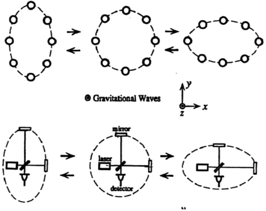
1-1 A passing gravitational wave's effects . . . . 1-2 Neutron star with a non-axisymmetric bump . . . . 2-1 LIGO interferometer ...

2-2 TCS system ...

3-1 Phase camera and galvo control loop . . . . 3-2 OMC in relation to the interferometer . . . . 3-3 Modal decomposition of OMC transmission . . . . . 3-4 Phase map generated from OMC model . . . . 3-5 Michelson bright fringe on transmission of the OMC 3-6 Direct reflection off ITMY on transmission of OMC . 3-7 Michelson bright fringe directly to phase camera . . 3-8 Direct reflection off ITMX directly to phase camera. 3-9 Qphase fit of Michelson bright fringe data . . . . 4-1 4-2 4-3 4-4 4-5 4-6 4-7 4-8

Carrier, sidebands and reference beam . . . .

Reference beam setup for the phase camera .

Carrier signal: horizontal and vertical profiles Fit of carrier on sideband signal .. . . .

"Reversed TCS" state images .. . . .

"No TCS" state images ...

"Tuned TCS" state images .. . . .

"Power up" state images .. . . .

5-1 Diagram of angles for precession . . . .

. . . . . 66 . . . . . 70 . . . . . 71 . . . . . 72 . . . . . 78 .... . 79 . . . . . 80 . . . . . 81

5-2 Precession for small A ... 5-3 Precession for small 0 ...

5-4 Ellipticity as a function of current frequency . . . . 5-5 1st Spin down as function of current frequency . . . . 6-1 Reference angles for definition of interferometer location .

7-1 7-2 7-3 7-4 7-5 7-6 7-7 7-8 7-9 7-10 7-11 7-12 7-13 7-14 7-15 7-16 7-17 7-18 7-19 7-20 7-21 7-22 7-23

RX J1856.5-3754: version 1 largest 2F values for H1 RX J1856.5-3754: version 1 largest 2F values for L1 RX J1856.5-3754: version 2 largest 2F values . . . . . RX J1856.5-3754: coincident largest 2F values . . . .

RX J1856.5-3754: upper limits . . . . RX J1856.5-3754: ratio of V1/V2 upper limits . . . .

Sensitivity scaling as a function of templates . . . . .

Confidence vs injection runs . . . . Strain vs SFT for all 3 interferometers . . . . Estimated strain vs frequency for all 3 interferometers

Gaussian noise strain vs SFT . . . . Estimated Gaussian noise strain vs frequency . . . . .

Expected versus actual number of templates for all 3 interferometers . . . .

Expected versus actual number of templates for a Gaussian noise data set . L1: weighted noise from 59 to 60 Hz . . . . H1: weighted noise from 59 to 60 Hz . . . . Distribution of templates with 2F greater than 25 for all 3 interferometers . Distribution of templates with 2F greater than 25 for Gaussian noise data . Response of the Hanford detector to varying 0 and i . . . . Response of the Livingston detector to varying O and i . . . . Confidence versus injected signal strength . . . . Ellipticity versus moment of inertia . . . . Ratio of GW energy loss to total spin down energy loss . . . .

95 96 101 102 107 . . . . . 127 . . . . . 127 . . . . . 128 . . . . . 129 . . . . . 131 . . . . . 132 . . . . . 135 . . . . . 138 . . . . . 140 . . . . . 142 . . . . . 143 143 145 146 148 148 150 151 154 154 155 157 158

List of Tables

3.1 OMC parameters ...

3.2 Astigmatic beam decomposition . . . . 3.3 Fit and model of OMC scan . . . . 3.4 Amplitude modulation comparisons . . . . 3.5 Model and fit comparisons for both the Michelson

reflection . . . . 4.1 NSPOB and sideband power ratios . . . . 4.2 Heating states and phase camera power ratios . . . 7.1 Crab parameters at the start of S5 . . . . 7.2 Positions of Hanford and Livingston detectors . . . A.1 Acronym definitions . . . .

bright fringe and direct 75 76 136 153 163

Part I

Chapter 1

Generating gravitational waves

This chapter describes gravitational waves and considers their generation from isolated neutron stars.

1.1

General relativity and gravitational waves

From the simple experimental observation of the equivalence of inertial and gravitational masses and the desire to incorporate the principle of relativity into a theory of gravity was developed one of the most elegant and successful theories of physics, that of Einstein's General Relativity [20]. It tells us that masses move along geodesics and that the curvature of space-time along which mass moves generates the perceived gravitational force. In turn space-time curvature is generated by the presence of mass and energy. This fact leads General Relativity to predict the propagation of gravitational waves on space-time [40].

Consider the curvature encoded in the space-time metric g,, where

ds2 _{= gdx} d x . _(1.1)

Here ds is the space-time interval or proper time of an observer who is at rest with the coordinate system, dxl and dxv are the indexed coordinates of space-time and the Einstein summing convention is assumed. From this most general case, let us consider the weak-field limit where space can be considered mostly flat with a small perturbation on top of it, which is a reasonable approximation to human scale laboratories on Earth. In this case the metric g,, can be written as

ggi = 7guj + h(,.

where h,, is the perturbation (and thus holds the gravitational wave information) and ,,v

is the Minkoski metric of flat space-time equal to -1 0 0 0

0 100

7/pv = .(1.3)

0 010

0 0 0 1

In order for a gravitational wave to propagate, it must satisfy the wave equation h

=

(V2

We neglect the static solutions to the wave equation, as we are interested in radiation which changes with time as opposed to static Newtonian potentials. We are free to choose the coordinate system in which to view the perturbation (gauge choice) and the one in which the math is most clear is the transverse traceless gauge, in which freely falling masses move along coordinate lines. In the transverse traceless gauge with the weak-field assumption, the solution of a wave propagating in the x3 direction can be written as [40]

00

0 0

0

h h 0

h, (x, t)

cos

0 hx -h

0

c

00 0 0 0

where h+ and hx are the two possible polarizations of the wave and

fGaw

1.1.1

Gravitational wave effects on test masses

Consider a h+ polarized gravitational wave acting on a pair of test masses at rest relative to each other. Place both a distance L from the arbitrary origin of their common Lorentz frame, one along the x1 axis and the other along the x2 axis. Apply the g,, metric to find

the space-time interval ds between the origin and each of the masses as a function of time.

As a h+ polarized gravitational wave propagates in the x3 direction, the ds between the

origin and the first mass will vary sinusoidally and be 1800 out of phase with the sinusoidal variation of ds between the origin and the second mass.

One method to sample this change in ds is to propagate a laser beam from the origin to each test mass and back. One can integrate along the laser's path from the origin to each test mass to find a measurable quantity, the difference in the light's phase between the two round trip paths:

L L

A = 2

Ig

dx

- 2-f Vlgxxlldx

(1.6)

0 0

where A is the wavelength of the laser light and A4 is the difference in total accumulated round trip phase by the laser light along the two paths. If the laser light round trip time is small compared to the gravitational wave period, then the maximum total difference caused by a h+ wave can be approximated by

2rL

a)

r

1.1.2

Generation of gravitational waves

To gain insight into the generation of gravitational waves, we look to electromagnetic theory as a guide. Electromagnetic waves are governed by the same wave equation except that the electromagnetic field E replaces the perturbation h,,. If we restrict ourselves to waves whose wavelength is much larger than the source we can use a multipole expansion. In the same way acceleration of charge is necessary for electromagnetic waves, acceleration of mass (and thus second derivatives of the moments) are necessary for gravitational waves. The monopole of the expansion for both electromagnetic waves and gravitational waves does not radiate due to the conservation of charge on the one hand and the conservation of mass and energy on the other. We can move on to consider the gravitational equivalent to the electric dipole [40]

b

I

SGmravitational

Waves

F

II

\

Figure 1-1: Effects of a passing gravitational wave on free masses and a laser interferometer.

• /

dg = p(r)rdxidx₂dx3 .

(1.8)

However, it is easy to see that the second derivative of dg will be zero because of the conservation of momentum (mr = constant). The next higher moments are equivalent

to the magnetic dipole and the electric quadrupole. The gravitational equivalent to the magnetic dipole is

Pg

=

v

Again in this case there is no radiation, this time due to the conservation of angular momentum (min x r = constant). Finally, with the quadrupole moment we lack any more

conservation laws to apply and thus have the first term in the expansion that can generate radiation. The typically quoted reduced gravitational quadrupole moment is

I

=

zX

Z

F,

Thus in direct analogy to electromagnetism's potential [35]

A = -- (1.11)

R

where di is a charge dipole moment and R is the distance from the dipole to the point where the potential is measured at, we can write

hJV = R

_Rp,.

Note that we are working in units where the gravitational constant, G, and the speed of light, c, are set to 1. The factor of 2 comes from the correct tensor calculations which are presented in detail in [40].

1.2

Continuous gravitational wave sources

For the majority of this thesis we will focus on one type of source of changing quadrupole moment, a non-axisymmetric isolated neutron star. One can imagine such a star with a bump on its surface or an equatorial bulge producing an eccentricity as shown in Figure 1-2. Consider a non-axisymmetric neutron star with the principle moments 111, 122, 133.

Let us assume it is rotating about the x3 axis with frequency fROT. In this case the second derivative of the quadrupole moment tensor IA, is [56]

I, =

0

-167r 2

f~OT (11 - 122) cos (47fROTt)

-321r 2 _fOT

_(I11

0

0

-327r 2f OT (/11 - 122) sin (47fRoTt) 1672fROT (11 - 122) cos (47rfROTt)

0

I1-122 can be replaced in the above with E133 by using the definition of equatorial ellipticity

Ill - 122 E = 133 (1.13) (1.14) "

Using this I,, in Eq. (1.12) and choosing to observe the generated wave from a new coordinate system with the X3 axis oriented at an angle i away from the axis of rotation we get [56]

0

0

0

0

327r2f,2tEI33

0

0

0

0

0

(1.15) This can be compared to Eq. (1.5) which allows one to read off h+ and hx and also note that fGW = 2

_fROT.

From the above Eq. (1.15) it is easy to determine what properties a detectable contin-uous wave source would have. First of all, it must have some eccentricity. However there are theoretical estimates of the maximum possible eccentricities supportable by neutron stars. These estimates are based off of possible equations of state for neutron stars, which are equations which define the relationship between the temperature, pressure and density within the star. By surveying the more plausible equations of state one finds a maximum ellipticity of - 10-6 [51] can be supported. Exotic equations of states for things such as hybrid or quark stars, where the core is partially or completely made up of quark matter, can have maximum ellipticities a factor of 100 larger. However, it should be noted that such equations of state are considered by many astrophysicists to be speculative, and so the ellipticities we infer from them may not be quite as plausible [42]. A more in-depth discussion of ellipticities of neutron stars is covered in Section 5.2.

Secondly, the source needs to be rotating rapidly, due to the f2 dependence of the strain. It also needs to be within the LIGO detection band, which has a low end. around 50 Hz determined by seismic noise. Known pulsars have a maximum spin periods of a few milliseconds, yielding maximum gravitational wave frequencies of about 1 kHz. In the case of an isolated neutron star this means it needs to be young and not have radiated away

too much of its angular momentum. Thirdly, an ideal source should be as close as possible since the strain at a detector is inversely proportional to the distance to the source.

By considering the known properties of neutron stars we can now make a quick estimate of the maximum strength of gravitational waves reaching detectors on Earth. Typical radii are of order 10 km and typical masses are around 1.4 M₀ [40]. This leads to a typical moment of inertia 104 5 g cm2 _{assuming a rigid rotator. Using 1 kpc as a distance standard} and simply note any change in distance just produces an inverse change in the detect strain. The above equations can be converted from natural units to experimentalist units by including correct factors of G and c. Using the typical maximum values for frequency and ellipticity yields a GW amplitude of the order h - 10-24(1 kpc/R) (/10- 6)(f/500Hz)2 detected at Earth from a source 1 kpc away.

Angular Momentum

Vector

7

Figure 1-2: Diagram of a non-axisymmetric neutron star with a bump. The angle i is the inclination angle between the axis of rotation and the direction to the detector.

Next we consider two isolated neutron stars that could make good candidates for detec-tion by LIGO.

1.2.1

_{Potential source: RX J1856.5-3754}

A potential candidate that meets several of the previously listed criteria is the isolated

neutron star RX J1856.5-3756. RX J1856.5-3754 is the closest known neutron star, at a distance of - 120 pcs [31] [53], as determined by parallax measurements. While it is seen in the optical by the Hubble space telescope, it was actually discovered in the X-ray by the Rosat All Sky Survey in 1996 [54]. It does not emit detectably at radio wavelengths,

and thus was not in the original set of pulsar candidates being examined by LIGO. It has a remarkably featureless x-ray spectrum which is well fit to a black body spectrum of temperature 63.5 eV, although there is an excess in the UV-optical region of the spectrum by about a factor of 7 from just the x-ray data fit [13]. A naive black body fit to the x-ray data suggests that the star is of the order 4km in radius while a similarly naive black body fit to the optical data leads to a star of radius of 14km [13]. The extreme mismatch between these two fits indicates that one must model the effects of the neutron star's atmosphere to understand the electromagnetic emission. At the time of considering RX J1856.5-3754 as a source Chandra and XMM observations had not been able to detect any periodic variation in the x-ray emission, having placed an upper limit of 1.5% on the pulsing fraction of x-rays relative to the total x-ray flux [12].

A lack of spin period to focus on requires a blind search, although there are good estimates of its age allowing us to limit the parameter space of the search, when coupled with spin down energy calculations. Since the star is losing rotational energy as it radiates away gravitational radiation, an equation relating the current rotation frequency and the rate of change of that rotation frequency (the spin down rate) can be written. If sufficient time has passed since the birth of the neutron star, such that the current rotation frequency is small compared to the rotation frequency at birth, the ratio between the current rotation frequency and the current spin down rate will become a function only of the age of the star. If the age is known then at any given frequency, spin downs only up to a certain maximum need be considered, limiting the spin down parameter space necessary to be searched. This is covered in more depth in Section 5.3.

Age estimates for RX J1856.5-3754 come from considering its temperature and how rapidly it cools, the lack of a visible super nova remnant, and possible associations with other stars from a common starting point. Its high temperature and x-ray brightness implies that RX J1856.5-3754 must be around 106 years old or younger, since the star has not lived long enough to cool too much by thermal emission. On the other hand, there is no visible supernova remnant, which implies an age greater than about 105 years, the length of time most supernova remnants remain visible. RX J1856.5-3754's proper motion of - 0.33 masyr- 1 suggests that - 5 x 105 years is correct. Tracing RX J1856's trajectory back in time finds it crossing the trajectory of run-away star ( Oph 5 x 105 years in the past [52]. They both may have originated in the Upper Sco OB association, where their paths meet,

before the supernova of the progenitor of RX J1856.5-3754 kicked them out.

While carrying out a gravitational wave search directed at RX J1856.5-3754 it was found to have a spin period below the LIGO detection band by X-ray astronomers. It has a period of 7 seconds with only a variation in the X-rays of 1.5%, the smallest ever seen in an isolated X-ray pulsar [50]. However the methodology and resulting test of the code and search pipeline performed using it as a target are still of use and thus it is presented here and in Chapter 7.

1.2.2

Potential source: the Crab pulsar

The Crab pulsar and its surrounding nebula are remnants of a supernova that occurred in 1054 AD approximately 2 kpc distant [17]. Its been well studied over a broad band of electromagnetic frequencies from radio to gamma rays [38]. It produces very regular pulses across the electromagnetic spectrum whose frequency and time evolution are known to high accuracy. These electromagnetic wave pulses provide insight into the rotation rate and spin down rate of the Crab pulsar and also act as a starting point from which to narrow down directed searches for gravitational waves from the Crab pulsar.

The Crab has a known radio pulse frequency of ~ 30 Hz which implies the rotation

frequency is close to that. It also known to be spinning down at the rate of - 3 x 10-10 Hz/s [38] [28]. This information lets us calculate a naive classical upper limit on the strain at an earth based detector of 1.4 x 10-24 and upper limit of 7.5 x 10-4 _{on the ellipticity}

of the Crab pulsar [43]. Thus the Crab is a good potential source because of its extreme youth and rate of spin down, despite its distance. These radio observations also let us narrow the parameter space down, but there is still some uncertainty left in how closely the gravitational radiation period matches the radio pulse period [56].

Chapter 2

Laser interferometer gravitational

wave detectors

This chapter will summarize the basics of a laser interferometer detector. It will then discuss heating problems with certain optics which arose while trying to reach the designed input laser power and how these problems were addressed with a thermal compensation system. An in depth examination of the laser light inside the interferometer from before and after this compensation system was used can be found in Chapter 4.

2.1

Laser interferometers

2.1.1

Introduction

One of the simplest and most sensitive methods for measuring the difference in length along two paths is a Michelson interferometer. Figure 2-1 shows the full Michelson interferometer combined with the two Fabry-Perot arms, discussed in Section 2.1.3 and a power recycling cavity, discussed in Section 2.1.4. This setup is the heart of all three LIGO detectors. These interferometers have been undergoing construction and commissioning for the past decade and recently have gone through several periods of designated data collection. These periods, during which the interferometer is left to simply run without constant upgrades and commissioning, are refered to as science runs. The most recent science run, the 5th SO

far, started in November 2005 and was the first science run in which the interferometers were operating at their designed sensitivity level.

At its most basic, a LIGO interferometer consists of a laser light source which is then directed through a 50/50 beamsplitter. The transmitted and reflected beams travel along perpendicular paths until reaching two end test masses (ETMs), which are highly reflective mirrors. The reflected light from each mirror is then recombined at the beamsplitter. The recombined electric field at the anti-symmetric (AS) port depends on the difference in the optical paths of the two beams. The electric field at the AS port for this simple configuration can be written as

EAs

=

Ein

(2.1)

where Ein is the electric field incident on the beamsplitter from the laser source, Ox and

¢y are the phases accumulated by the light in a one way trip down each arm, tbs and rbs

are the field transmission and reflection of the beamsplitter, and rex and rey are the field reflection of the end mirrors [3]. In reference to the earlier calculations in Section 1.1.1, the A,1 of Eq. (1.6) would be equal to 2(%y - Ox).

2.1.2

Laser and mode cleaners

The main laser is a 10 Watt Nd:YAG laser from Lightwave, which operates at a wavelength of 1064 nm. It is both frequency and intensity stabilized. The laser output is passed through a pre-mode cleaner (PMC). This is a 21 cm long triangular cavity designed to filter the spatial mode and intensity noise above about 1 MHz. It then passes through the mode cleaner, another triangular cavity, with a 24.492 meter round trip. This cavity spatially filters the light, only allowing a single mode to pass, while higher order modes pick up additional phase and fall out of resonance. It also acts as a stable angular reference, as misalignments become translated to higher order modes within the cavity and also fall out of resonance [3].

2.1.3

Fabry-Perot arms

To increase the sensitivity of the basic Michelson interferometer, one would like to increase

L, the length of the arms, up until the length is comparable to the wavelength of the

gravitational waves, roughly 300 to 6000 km. At that point the approximations leading up to Eq. (1.7), which shows the signal grows linearly with L, break down. Effectively,

Pickoff

Port

BS

Ii

AntETMi-

Anti-Symmetric

Port

Figure 2-1: A diagram of a LIGO interferometer (taken from [3]). The purple light repre-sents the input laser light. The blue line reprerepre-sents the resonant sidebands in the power recycling cavity while the red line represents the carrier signal resonant in the recycling cavity and the Fabry-Perot arms, as discussed in Sections 2.1.3,2.1.4, 2.1.5.

the light is picks up phase shifts from multiple cycles of the wave which cancel each other, preventing any further gain in sensitivity. There are technical problems with building the arms even 300 km long. One way to effectively make the arms longer is to have the laser light make multiple trips down the same arm. As long as the time spent by the light in the cavity is small compared to the period of the gravitational waves, this will significantly increase the sensitivity of the instrument. However for changes occurring faster than this storage time, the resulting signal will be attenuated relative to the lower frequencies in the same configuration.

By turning the Michelson interferometer arms into resonating Fabry-Perot cavities, one can increase the number of round trips the laser light makes. This adds technical complexity in the form of an additional set of partially transmitting input test masses (ITMs) and the

Port

Inp

-f

Be

fl4

F~R

I

&EE4

necessary feedback control systems to keep the Fabry-Perot cavities on resonance.

2.1.4

Power recycling cavity

In the case of the Michelson interferometer, the light interferes destructively in the direction of the AS port and constructively in the direction of the incoming laser light. Instead of just dumping the outgoing power, one can construct a cavity to take the outgoing light and recycle it back into the interferometer. By adding a partially transmitting recycling mirror between the laser and the beamsplitter a cavity can be made which recycles the power back into the interferometer. This cavity also requires additional feedback control systems to remain on resonance and generally provides a factor of 50 gain to the carrier, and a factor of 26 gain to the sidebands when the input test masses are thermally tuned [5]. The recycling mirror transmission was chosen to match the total round trip losses by the carrier in the rest of the interferometer so as to couple all the carrier light into the interferometer [3].

The reason for using all available power is because of shot noise. The interferometer operates on a dark fringe and thus very few photons carry the gravitational wave signal to the AS port. Shot noise is due to the quantum fluctuations in the number of photons reaching the detector. Shot noise scales as sqrtN, where N is the number of photons. However, the gravitational wave signal scales with the power. and therefore the number of photons, and so the signal to shot noise ratio scales as sqrtN [3]. By increasing the total power we increase the interferometer sensitivity at the frequencies which are limited by shot noise.

2.1.5

AS port

The electric field at the AS port is detected with a photodiode, which produces a photo-electric current proportional to the average photon flux, or power, on the detector. For a simplified calculation of the power at the AS port we assume the end mirrors have identical reflectivity and are equal to 1 (i.e. re = ry = re = 1) and that the beamsplitter is a perfect 50/50 (i.e. rbs X tbs = 1/2). Using Eq. (2.1) we can then write the AS port power as

PAS= E*E = 4IEin12(retbsrbs)2 sin(A )2 = IEi 2

where we define AL = 0y - ¢z [3]. To produce signals that are at radio frequencies on the photodiodes, the light entering the interferometer is first phase modulated to produce several sets of sidebands. These sidebands are used in a Pound-Drever-Hall locking scheme [18] (see also [23]), to keep the different cavities on resonance (or locked). One set of sidebands is reflected by the mode cleaner, one set is reflected by the power recycling mirror, and the last set is reflected by the input test masses, and resonate in the recycling cavity. This last set of sidebands which resonates in the power recycling cavity is used to beat against the carrier and produce the final gravitational wave signal channel at the AS port. An asymmetry of 0.356 m in the lengths between the BS and the two ITMs, called the Schnupp asymmetry, causes the sidebands to come out the AS port. Nominally, the recycling cavity should be almost critically coupled for the sidebands such that almost all the sideband light should end up at the AS port.

These sidebands are produced by using a Pockels cell to phase modulate the input light. The laser light modulated once for one set of sidebands can be written as

Ein = Eoeir cos(nmt)

- Eo(Jo(F) + iJl ()e +immt + iJl(F)e-i 'mt (2.3)

_ J

(r)e+i

mT _ J

(r)e-i

_mt)

(2.4) where F is the modulation depth in radians, Qm is the modulation angular frequency, Jn is the nth order Bessel function of the first kind, and Eo is the unmodulated field of the laser. In the case of the sidebands resonant in the power recycling cavity,

Qm

2.2

Problems

2.2.1

Thermal heating and thermal compensation

The ITMs were designed with the concept that a certain amount of absorption would be taking place leading to a curvature change due to thermal lensing, effectively the changing index of refraction due to increasing temperature, when operating in a high input power (6 Watt) state. The power gain of 50 in the recycling cavity and gain of 130 in the arms means roughly 300 W and 10 kW are circulating in the recycling cavity and arms, respectively, in this high input power state. The expected absorption was about 1 ppm in the HR coating and about 4-5 ppm/cm in the substrate. Through the initial science runs, during which the LIGO interferometers were left alone to take data as opposed to being worked on directly to improve sensitivity, the LIGO interferometers were operating below this expected high power state and consequently had a slightly wrong radius of curvature for the ITMs and ETMs.

However, during attempts to reach high power on the H1 interferometer, it became clear that optics were absorbing far more then expected. At their nominal radius of curvature at 6 Watts of input power, the gain in power in the sidebands is theoretically expected to be Gsb = 30 [5]. However, a maximum gain of Gsb = 26.5 was measured at 1.8 Watts of laser power into the mode cleaner, a much lower power than expected. At higher power, the sideband power gain reduced along with the sidebands decreasing in spatial size. This suggested that one or more optics of the power recycling cavity was absorbing too much power.

Using spot size measurements on H1 at different IFO ports and at different heating states [41], we were able to determine that ITMX was absorbing the most power, 34 ± 4 mWatt per Watt of power into the mode cleaner, although ITMY was only a factor 2.6 less than that. These in vacuum measurements were unable to distinguish between bulk substrate absorption or coating absorption. However, since the power hitting the first coating layer on the high reflectivity side of the ITM, which faces the Fabry-Perot arm cavity, is roughly 140 times the incident power, and the higher probability of surface contaminants, the absorption is most likely due to the surface rather than the bulk. If one assumed all the absorption were in the surface, then the ITMX coating would be absorbing 15±1.8 ppm and the ITMY coating would be absorbing 5.6 ± 0.7 ppm. This is compared to the specification of 1 ppm.

One hypothesis is that contaminants were introduced to the surface during assembly and installation and resulted in this large difference from specification to the actual absorption. However, we don't have a definitive cause of the excess absorption. Based on these findings, ITMX was replaced with a spare in June of 2005. Since the ITMs still had absorption values above the design specifications, a system was necessary to compensate for the thermal heating effects of the main laser.

A thermal compensation system (TCS) was originally studied by Ryan Lawrence [36] and was designed to apply heating to the test masses as needed to correct the curvature. This eventually led to the full system installed on the LIGO interferometers [48] [6]. The final systems installed for each ITM, shown in Figure 2-2, consist of a 10 Watt C02 laser operating at 10.6 ym wavelength that illuminates one of two interchangable mask patterns. The laser light passes through a telescope with magnification of 26.5 and a ZnSe viewport before reaching the high reflectivity side of the ITM (the side facing the arm cavity) of the ITM. The 10.6 pm laser light is almost completely absorbed by the fused silica substrate of the ITM.

To ETM

BS

High

Reflectivity

Surface

Annulus Mask

Over-heat

Correction

Hole Mask

Under-heat

Correction

Figure 2-2: A schematic of the Thermal Compensation System (TCS). This was installed on both ITMs on all 3 LIGO interferometers. It is made up of a 10.6 Jm CO₂ laser, a set of

interchangable masks, and a series of projection optics that produce an image of the mask on the optic.

ZnSe

Viewport

The two masks are an annulus pattern and a hole. The annulus is used to compensate for too much heat being deposited by the main LIGO laser light. The hole in the center is used to correct for insufficient heat to reach the desired curvature. These masks are installed in the Fourier plane of the projection system. A Bessel mask further downstream clips the higher order maxima of the Airy diffraction pattern, leaving only the central lobe of the Airy disk. A polarizer on a rotation stage is used to adjust the power.

This system was successfully able to correct for the high power heating effects and allowed the LIGO interferometers to reach operation at 6 Watt input laser power state. To control the long time dependence of the TCS on the radius of curvature, a servo system was devised and implemented. The full details of this system can be found in Stefan Ballmer's

thesis

[5].

2.2.2

Mode and power mismatches and the

AS_I

signal

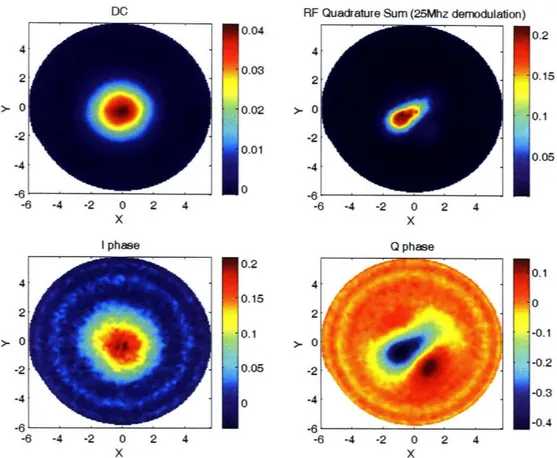
The carrier light resonates mostly in the 4 km long arms of the interferometer, and thus their spatial mode is mostly dependant on the state of the arm cavities. The sidebands only resonate in the power recycling cavity and thus the sideband structure is determined by the state of the power recycling cavity. The deformation and thermal lensing of the ITMs, due to their excess absorption, affects primarily the power recycling cavity. This causes the two sidebands' power and spatial profiles to become mismatched with the carrier and each other. Since the gravitational wave signal is detected by the beat between the carrier and sidebands, poor matching will lead to excess noise.

To illustrate what poor matching can do, we write the incident light field on the AS photodiode as

T = Ace- i ct + iA+e-i(wc+n•)t + iAe -_i(W' -_{c~ )t (2.5)}

where Q1m is the sideband modulation frequency, wc is the carrier frequency, and Ac, A+, A_

contains the modal content and the relative magnitudes of the carrier, upper sideband, and lower sideband respectively. When the photodiode signal is demodulated at frequency

Qm, two signals are produced, the In-phase signal and the Quadrature-phase signal. Since

these are recorded by the AS port photodiode, these are labeled ASI and ASQ. The interferometer is designed such that gravitational wave signals are only in AS_Q and the

ASI signal is zero.

We can write the power in each demodulated signal as

27,

PASJ = j m - * cos(Qmt) = (AcASb+ + A*Asb-) - (AAsb+ + AcAb

(2.6)

and

PASQ = jm V* sin(Qmt) = (AcAsb+ + A*Asb-) + (A *Ab+ + AcAb_) (2.7)

where PASj and PAS_Q are the powers in the ASI and ASQ signals.

Note that when the sidebands have identical amplitude and modal content, namely

Asb+ = Asb-, PASI goes to zero, leaving only AS_Q with signal. However, if the overall

magnitude is different, effectively amplitude modulation of the sidebands, PASa no longer identically cancels. In addition if the modal content of the sidebands are not identical, and there are higher order modes present to beat with in the carrier, PASJ will again not cancel. The higher order modes in the carrier and sidebands will also add noise directly to the ASQ signal as well.

If the mismatches between the carrier and sidebands are severe enough, the excess ASI signal can cause saturation of the RF electronics and mixers, resulting in loss of any gravitational wave signal [3]. There is an electronic system in place to provide feed-back that cancels out RF photo current on the diode caused by the ASI signal. This system can correct up to 10 mApk photo current per diode. The control signal for this system is recorded in the channel ASJCorr. However in high power configurations this correction system proved to be insufficient [5]. The excess ASI problem was eventually solved with the thermal compensation system running a correction servo designed to null the ASi_Corr signal. It is important to examine the power and modal nature of the individual components of the light in the recycling cavity with and without TCS correction, to ensure that it is correcting properly. This examination is accomplished through the use of the phase camera, a system whose basics and initial test case are described in Chapter 3. The examination of the thermal states and TCS correction of the interferometer is covered in Chapter 4.

Part II

Chapter 3

The phase camera: a frequency

sensitive wavefront sensor

The "phase camera" is a high-resolution wavefront sensor that measures the complete spatial profile of any frequency component of a laser field containing multiple frequencies. This technique is useful as a probe of the spatial overlap of the carrier field with each sideband component exiting the output port of a gravitational wave interferometer. It was first demonstrated to work at MIT [25] and then brought to the LIGO sites.

This chapter describes the functioning of the phase camera at a basic level, where it detects only the beat signal between the carrier and sidebands. At the Hanford site, the phase camera was first successfully used to test an output mode cleaner and confirm that it was working as designed. That test is presented here to show the phase camera working in a relatively simple to understand case on the actual interferometer. The addition of an independant reference beam, described in Section 4.1.1, was necessary for the more complex study of individual sideband and carrier components in different heating states described in Chapter 4.

3.1

Mechanical details

The phase camera is the combination of a position scanning galvanometer and a New Focus 1811A RF photodiode. The galvanometer moves two mirrors in conjuction such that the incoming light reflects off both in a spiral pattern and onto the photodiode at a rate of about one full spiral scan every half second. The two output channels of the photodiode,

DC power and RF power, are then sampled at a rate of up to 4000 points per full scan. The RF sampled points are then demodulated and passed to a computer, along with the position read back of the galvanometer as shown in Figure 3-1. The demodulation can be done at a frequency of 24.5 MHz, the difference between the carrier and sideband frequencies, and thus looks at the beat between the carrier and sidebands of the incoming light. A reference beam can be combined with the incoming light to produce beats with the carrier and sidebands individually, allowing their individual demodulation, and which is described in Section 4.1

M

lated

Computer Display

and Control

Spiral Scan

Position

2

I

ge

Figure 3-1: Phase camera control setup. The galvanometers move a pair of mirrors, directing the light in onto an 1811A RF photodiode. The RF signal from the photodiode, produced when the carrier and RF sidebands beat at 24.5 MHz, is demodulated, and then sent to a computer, along with the DC signal, where the signals are recorded. The computer sends the signal for the next position to a digital to analog converter board, which converts the signal into a control voltage which moves the mirrors to the next point in the spiral pattern.

3.2

Testing the phase camera and the output mode cleaner

The phase camera was used to help test and understand an output mode cleaner (OMC) on the Hanford 4km interferometer [10]. This also presented an opportunity to test the phase camera itself, to ensure that it was operating as expected.

3.2.1

Motivation for the output mode cleaner

Laser interferometers have problems associated with imperfect interference at the AS port, due to poor beam quality. Excess carrier light in higher order modes will produces excess shot noise while not contributing to the signal. Imperfect matching in the reflectivity of the two arms will produce a static, TEMoo carrier field at the AS port, which when it beats with the sideband light will produce noise in the signal channel. Any sideband field which does not spatially overlap with the carrier does not contribute to increasing the optical gain, but rather produces many detrimental effects like shot noise, acoustic sensitivity and so forth [3].

A potential solution to poor output beam quality is to place an output mode cleaner in the path of the AS port light before it reaches the AS photodiodes. By using a cavity with sufficiently large line width, both the RF sidebands and carrier TEMoo modes could be transmitted on the same resonance, while passively rejecting the higher order spatial modes. The more recently adopted solution is for future upgrades to the LIGO interferometers is to use only carrier light, without RF sidebands, a so called DC readout.

Experimental setup

The OMC was placed on the AS port of the Hanford 4k Interferometer as shown in Figure 3-2. This OMC was a solid spacer triangular cavity with a piezo-electric transducer (PZT), a device which converts electrical field into length changes, attached to one mirror for length control. It was designed to pass the TEMoo carrier and sidebands through the same0 0

resonance, while rejecting all the higher order modes. The cavity was held on resonance by applying a small dither signal to the OMC length at 40 kHz, and using a lock-in amplifier to generate an error signal from the transmitted light. A few useful parameters of the OMC are shown later in Table 3.1.

Incoming light

We have modeled and taken data for the OMC in the two simplifying cases of the laser reflected directly off an ITM onto the AS port, and of the interferometer being held on a Michelson bright fringe with the RM and ETMs misaligned. In these cases we assume that the modal content of the incoming carrier and sideband is essentially the same. However, a beam scan of the light on the table showed the light to be astigmatic, complicating the situation. The light had a first beam waist of 137pm along an axis rotated 250 counterclock-wise relative to the OMC horizontal axis. The second beam waist of 107pm located 6.6 cm after the first waist was along an axis rotated 250 degrees relative to the OMC vertical axis. Initially, the OMC was mode matched to only the horizontal waist, treating that as the only waist. However, during the testing process it was moved such that the transmission through the OMC was maximized. All data present here is from this later situation.

Phase camera

In this experiment a 50/50 beamsplitter was placed at the output of the OMC, redirecting half of the transmitted light to the phase camera. On the path to the phase camera, shown in Figure 3-2, two lenses were placed so as to focus the light to the proper size to be scanned. This means the phase camera photodiode was approximately 0.45 m from a waist size of 150pm, resulting in a Gouy phase of nearly 7r/2 radians. The Gouy phase is the phase difference between a Gaussian beam and a plane wave of the same optical frequency, acquired by the Gaussian beam as it propagates through a focus. This effective phase shift is different for higher order modes,

3.2.2

Theory and modeling

In the following sections a model for the astigmatic light from the interferometer reaching the OMC, and then passing through the OMC, will be developed. This requires defining a basis of modes affected by astigmatism, then transforming it into the OMC basis. By comparing the relative power in the modes actually measured at the output of the OMC with what we can determine if the OMC was built properly and performing as we expect.

Astigmatic beam

The Hermite Gaussian basis provides a complete set of solution for the fields which can propagate inside or outside of the cavity [33]. These solutions for the electromagnetic field,

4', which have been normalized for power, have the form

T mn = n)Hm Vx Hn

2(m+n)m!n!r (z) () w(z)

x e(x2+y2 )/w2(z) e-ik(x2+y2)/(2R(z)) eikz ei(m+n+l) tan-' [(zA)/(rw)]

(3.1) where m and n are TEM mode numbers, x and y are the distance from the center of the beam perpendicular to the direction of propagation, z is the distance from the waist in the direction of propagation, w(z) is the radius of the beam at z, w0o is the radius at the waist,

R(z) is the radius of curvature of the beam front at z, A is the wavelength of light, k is the

wave number (27r/A), and Hm is the Hermite polynomial of order m.

This can be generalized for the incoming light by breaking up the symmetry between the x and y axes and allowing them to have different waists and waist positions. In the case of a Michelson locked on a bright fringe and also a direct reflection of the laser light off an ITM, the light should be a pure TEMoo, distorted only by the astigmatism. Thus, the incoming light can be written as

astigmatic(X, y', z') = 2(m+m!n (Z) W

x

Hm

(Zx)Hn(

_(3.2)

x e- [x/wx(zx)]2-[/wY(zy )]2 eik[(zx+ z v)/2]

Sei[m+(1/2)] tan- [(z•A)/(wW2)] ei[n+(1/2)) tan- [(z2)/(Trw2)]W

where zx and zy are the distances from the x aligned waist wox, and the y aligned waist

The OMC basis

The OMC cavity imposes several boundary conditions on the general Hermite Gaussian solutions of Eq. (3.1). First, for resonance to occur, after each full round trip the phase and amplitude must match. Second, at the curved back mirror the wave front of the beam must match that of the cavity (neglecting the small incidence angle). Also note that, because of symmetry, the waist of the beam inside the cavity must occur midway between the two flat mirrors and equidistant from the curved back mirror. These conditions imply

= - ) 2 L(Ro - L) (3.3)

and

S(q

+ 1) +

Avo

where L is half the round trip length, Ro is the radius of curvature of the back mirror, Mod₂ is modulo base 2, and vo is the free spectral range (FSR). The FSR is equal to c/2L, where c is the speed of light, and is simply the distance in frequency space between successive transmission peaks of a given spatial mode. These transmission peaks are numbered by the q parameter, since q+ 1 is the number of half wavelengths inside the cavity. The modulo base 2 term comes from the fact that the cavity is triangular, and that for odd mode numbers in the direction parallel to the mode cleaner plane there is an additional 7r phase shift in the round trip )due to an odd number of reflections in the horizontal plane). Table 3.1 provides the values for these and several other related parameters of the OMC.

Table 3.1: OMC parameters

Cavity Finesse 30 Half of Round Trip Path (L) 50.75 mm End Mirror Radius of Curvature (Ro) 75 mm

Free Spectral Range (vo) 2.95 GHz Beam waist inside the OMC (wo) 109pm

Wavelength of Carrier light (A) 1064 nm

The important part of Eq. (3.4) is that for a given frequency of light, each (m + n) needs a different length of cavity to resonate, due to the Gouy phase shift. This means the OMC will decompose the incoming light into the Hermite Gaussian basis specified by its

geometrical parameters, and only let those modes whose (m + n) satisfy Eq. (3.4) to pass, generally the carrier TEMoo mode. All others will be reflected back from the OMC. However, because the mirrors of the OMC do not have perfect reflectivity, the range of frequencies which can pass is broadened, allowing most of the sideband TEM0oo modes to pass. This

can be seen by looking at the transmitted light of the OMC, considering the reflection and transmission at each mirror. Assuming no losses in the cavity and no transmission on the end mirror, the complex amplitude of the transmitted light will be

2transmitted - 1 t2incident i (3.5)

1 - rTr ₂

where

=2kL- 2(m + n + 1)cos- 1

1

tl = t2 represent the transmission of the mirrors, rl = r2 represent the reflectivity of the

mirrors, and assuming t? + r? = 1, for i = 1, 2. The k represents the wavenumber of the light and varies due to the 24.5 MHz frequency difference between the carrier and sidebands, resulting in a different transmission ratio for the carrier and sidebands of the same spatial mode.

Decomposing into the OMC basis

In order to understand how the astigmatic beam of Eq. (3.2) passes through the OMC, we need to decompose it into the Hermite Gaussian basis of the OMC, Eq. (3.1). This was done in two ways, both of which resulted in the same decomposition. The first decomposition was done by taking the inner product between the astigmatic beam and a particular OMC mode, essentially the inner production between Eqs. (3.1) and (3.2). This inner product,

J

The other method of decomposition started with creating a set of theoretical data with Eq. (3.2), with the amplitude of the astigmatic beam stored at a series of x and y coordi-nates. The simple model of

aooeioo00oo + aolei ~'o01 °

+

where Tmn is the mrnn th OMC mode, was then fit to this artificial data set. The amplitude

and phase of each of the modes (defined by Eq. (3.1)) is then left as a free parameter of the model. After fitting, we normalize the model by scaling so that the TEMoo00 mode has an

amplitude of one and a phase of zero. This second method is very similar to the one used to analyze the phase camera data. The results of the two decompositions are presented in the first two columns of Table 3.2.2. The matches between modes from the two methods are good, within ±0.02 in amplitude and ±110 in phase.

There are two additional decompositions which can provide insight, that of an astigmatic beam without the 25' of rotation, where the two waists axes are aligned with the OMC axes, and that of an astigmatic beam misaligned in vertical displacement coming into the OMC. In the first case, the TEM11 mode completely disappears, leaving only the expected TEM02 and

TEM20 modes due to the mode mismatch. In the second case a vertical displacement of one

third the waist size of the OMC was somewhat arbitrarily chosen because of measurements indicating alignment drift of this size on short time scales. This decomposition gives a feel for what deviations to expect between the OMC model and the phase camera data. The differences are mostly on the order of 15% for modes that are present in the perfect alignment and the inclusion of several misalignment modes, such as the TEM0 1. Table 3.2.2

summarizes all of these decompositions.

Lastly, to calculate the effect of the astigmatic beam on transmission of the OMC, one simply needs to apply Eq. (3.5) to each mode for both the carrier and sidebands, then add all the modes back together for the carrier or sideband.

Decomposition versus Michelson bright fringe OMC scans

One straightforward experimental test of the astigmatic decomposition is to tune the OMC's length such that modes other than the TEM00 become resonant and note the power of the transmitted light. In practice this is done by applying a slowly increasing voltage to the OMC's PZT to change the length of the OMC while continuously recording the power of