A diquark interpretation of the structure and energies of hadrons

A Diquark Interpretation of the Structure and

Energies of Hadrons

by

Alexander Selem

Submitted to the Department of Physics

in partial fulfillment of the requirements for the degree of

Bachelor of Science in Physics

at the

MASSACHUSETTS INSTITUTE OF TECHNOLOG

June 2005

LIBRARIES

©(

Alexander Selem, MMV. All rights reserved.

The author hereby grants to MIT permission to reproduce and

distribute publicly paper and electronic copies of this thesis document

in whole or in part.

Certified by...

Frank Wilczek

Professor of Physics

Thesis Supervisor

A ccepted by.

...-...

...

...

Professor David E. Pritchard

Senior Thesis Coordinator, Department of Physics

A/RCHIVES

Author ...

. ./4 . . . .

A Diquark Interpretation of the Structure and Energies of

Hadrons

by

Alexander Selem

Submitted to the Department of Physics

on May 20, 2005, in partial fulfillment of the requirements for the degree of

Bachelor of Science in Physics

Abstract

I present a simple phenomenological model which successfully organizes and classifies

essentially all hadrons. The model is originally inspired from three simple theoretical indications including: treating baryons as a two body system with a diquark and quark connected by a flux tube, thereby indicating that they lie on Regge trajecto-ries; allowing for independent combinations of diquark and quark to enumerate the observed trajectories; and that spin-flavor symmetric diquarks are more massive than their antisymmetric counterparts. With this framework essentially all hadrons can be consistently organized confirming the first three hypotheses and elucidating new ones, including: a universal slope or flux tube tension for both baryons and mesons implying the same color-charge at the flux tube ends, small spin forces external to diquarks, and the existence of tunneling effects. This framework and classification can then be used to estimate diquarks masses, and can be applied to exotic and cryp-toexotic states. The model also make predictions for the existence of several particles and their energies; among them, tetraquark states. Finally, the arguments presented here naturally lead to many future projects in both experiment and theory.

Thesis Supervisor: Frank Wilczek Title: Professor of Physics

Acknowledgments

This work is the fruit of a collaboration with Frank Wilczek, and many of the ideas

developed here were done so in conjunction. As my supervisor and mentor, I am most

grateful to him for all the guidance, help, and wonderful exchange of ideas through countless conversations we have had.

I would also like to especially thank Robert Jaffe for many helpful discussions, and

insights. I also benifited from discusions with Carlos Nufiez, Anthony Tagliaferro, and Barton Zwiebach.

This work was supported in part by the Paul E. Gray Endowed Fund, and I thank all those who have generously contributed to it.

Finally, I thank my family and God from which everything good has come.

Contents

1 Introduction and Background

1.1 Summary of the Uncorrelated Quark Model and Hadron Dynamics in

Practice

...

2.1 Classifying Diquarks ...

2.2 Motivations and Initial Hypotheses ... 2.3 Developed Hypotheses ...

2.4 Explanations of the Hypotheses ...

2.4.1 Generalization of the Chew-Frautschi Formula ...

3 The Classification of Particles

3.1 Methods ...

3.2 The Light Baryons ... 3.2.1 Nucleon-Delta Complex 3.2.2 Other Light Baryons . . 3.3 The Light Mesons ...

3.4 Exceptional Cases ... 3.5 Heavy Quark Hadrons ...

3.5.1 Application to Exotics . 3.6 Even-Odd Effect and Tunneling

4 Diquark Masses and Applications to Cryptoexotic States

9 10 13 14 16 19 20 21 27 . . . . 27

...

.30

...

.30

...

.34

...

.40

...

.42

...

.43

...

.45

...

.46

4.1 Cryptoexotica . . . 57

5 Conclusions, Future Directions 61

Chapter

1

Introduction and Background

The traditional quark theory of hadrons might be summarized as having two main inseparable components. The first describes the constituents of hadrons as being

sub-particles or quarks, as advanced by Gell-Mann in 1964 [1], while the second component

is the theory describing how these interact, namely the relativistic field theory known as Quantum Chromodynamics (QCD). Each is elegantly and well described, and yet

in practice this hardly seems to be the case. In what follows, I shall give a very brief

summary of this practice as related to this work.

The rest of the work and the main goal of this thesis will be dedicated to advancing a model where objects called "diquarks" are elevated to play a central role in thinking about hadrons. In particular I shall first describe the motivations for diquarks, their implications in phenomenology and how well the experimental data supports these

ideas. In doing so we shall find that a few simple hypotheses can be used to compactly classify essentially all hadrons, and give good predictions of their energies. Finally

I shall discuss the many fruitful elaborations and extensions that arise from this classification and the diquark model in general.

Many of the ideas presented in this work will also elaborated upon in a work to

1.1 Summary of the Uncorrelated Quark Model

and Hadron Dynamics in Practice

As dictated by quantum field theories in general, the true structure of the hadrons is

probably a "sea" of light quarks and massless gluons coming and going out of existence

mediating the interaction of what are called valence quarks or those which are the minimal number necessary to define a given bound state or hadron. In terms of the sub-particle components of the hadrons, however, one can just think of the valence quarks as being the constituents of the hadrons, and take the rest to be part of the interactions between these. The quarks have colors, r, b, g (an SU(3) symmetry),

spin (an SU(2) symmetry), and flavors u, d, s, c, b, t, (which can be thought of as a

very badly broken SU(6) symmetry, or an approximate SU(3) symmetry formed by u, d, and s). Because of the symmetry breaking in flavor it is sometimes intuitive

to think of quarks of different flavors as inherently different. Yet being fermions, we

must worry about symmetry under exchange, and in this regard flavor is treated as a perfect symmetry.

Mesons are (typically) described by a quark-antiquark pair (qq), while baryons

by three quarks (qqq). Most generally, any qqqlq combination is allowed as long

as nq - nq = 0 mod 3, where nq is the number of valence quarks present and nq

antiquarks present. This is required by an empirical and theoretical (via asymptotic

freedom) fact that all observed objects must be color singlets. In the traditional

quark theory, the quarks in the hadron ground state are each in their lowest state, and particle excitations proceed by exciting each of the quarks one at a time. Finally, the quarks having spin, requires us to ensure that Fermi statistics are obeyed. In mesons, because the antiquark is inherently a different particle than the quark, issues of symmetry under exchange need not be considered. However, as baryons are made of "identical" quarks (here flavor symmetry is taken to be exact), we must have that

Icolor) x flavor) x spin) x Ispatial) be antisymmetric, where the ket refers to

the whole baryon wave function, or the combined wave function of its three quarks.

x spin) x spatial) to be symmetric. The symmetry of the spatial part is denoted

by the particle's parity. The traditional quark model puts all quarks in the lowest excitation mode, where each has a positive or even parity while the antiquarks are given negative or odd parity. Baryons in their ground state, therefore, have even parity relative to the proton. Each quark (or antiquark in mesons) can then be separately excited by putting it in a higher energetic mode, having no effect on its parity, or by increasing in orbital angular momentum. Orbital excitations affect the

parity according to P = (-1)L, where L is the orbital angular momentum of the

state. For mesons another important quantity is charge conjugation C, given by

C = (-1)L+ S, where S is the total spin of the particle.

As mentioned, QCD is the theory that then describes how these quarks interact. The quark theory without QCD can only at best enumerate the states and quantum numbers of hadrons, but nothing can really be said as to the masses of the hadrons themselves or any other observables. Interesting predictions are only made when the dynamics of the quarks are taken into account. However, to date, no one has yet been able to systematically solve the QCD Lagrangian to produce an accurate description for the bound states of the quarks-namely the hadrons. Instead our true theoretical tests of QCD come from numerical super-computer calculations, which have been done in special cases; among these the ground states of observed

hadrons-which are in remarkable agreement with experiment (for example see Ref. [3, 4]),

thereby justifying our belief in the fundamental theory.

But this hardly suffices as a substitute for our understanding of hadrons. Instead many models have been employed in an attempt to dynamically describe hadrons. First there are non-relativistic potential models which treat the quarks as non-relativistic

bodies in a potential governed by the Schr6dinger equation [5, 6, 7, 8]. Typically a

Coloumbic plus linear potential is used, V(rij) = -a/rij + bri, where ij refers to any two quarks. It is a wonder that this program works even for the light quarks, as they are thought to have masses on the order of 100 MeV, which is comparable to the QCD coupling constant of 200 MeV, thereby requiring a proper relativistic treatment

made in these models attributed to relativistic affects helping to make them more plausible and better predictors.

The opposite approach is to treat the quarks as completely relativistic. This is the essence of bag models which place quarks in a "bag" with various boundary conditions

and degrees of freedom depending on the sophistication sought (for example [10, 11,

12, 13, 14, 15, 16, 17, 18, 19]). In these models, the vacuum exerts pressure B

("the so-called bag constant") on the bag providing for confinement, and the quark wave functions are then determined by solving the Dirac equation. Of course in practice, "bags" sometimes amount to spherical static cavities or other simplifications

[11, 12, 14, 15, 16, 17].

Finally, another simple phenomenological model is that of the flux-tube or

string-like model, used for mesons with orbital angular momentum [20, 21]. Here the QCD

force between the quark and antiquark is approximated by a string, or flux tube acting like an effective string, with some constant tension connecting the quark and antiquark. Most importantly, this model naturally reproduces experimental data and

lattice calculations [22, 23] where the energy squared of a particle, E2, plotted against

Chapter 2

The Case for Diquarks

Most generally a diquark is a two quark system. Because of confinement, it cannot exist in isolation, but rather might exist in combination with other quarks to form a bound color-antisymmetric state. For example, a baryon, being thought of as a diquark paired with quark, is the simplest example where they might exist. The idea of diquarks is probably as old as the quarks themselves. Gell-Mann makes mention

of their possible existence in his original paper on the quarks in 1964 [1], and since

then there has been a vast literature where people have used many models of hadron

structure employing diquarks. I refer the interested reader to a nice review given by Anselmino [24]. Briefly, I will mention some of the most salient points. One ex-treme view, is where a diquark is thought of as a point particle. This view implies

firstly that the various non-spatial parts of its wave function must be anti-symmetric between the two quarks that form it, and secondly it is treated as having no

inter-nal structure. But a much less stringent idea of a diquark, is simply one where two

quarks are said to be "correlated". In the literature the most general definition of a

correlation focuses only on a spatial criteria whereby a diquark is simply two quarks

whose mean distance is smaller than the mean distance with any other quarks in the particle. However, another interpretation of "correlation" is one where the diquark

wave function is separately antisymmetryzed as in the point-like conception of a

di-quark, but still assuming the diquark to be an object containing the structure of two quarks with some separation. This is the view assumed in this thesis. We think of

a diquark as an internal component of a particle, having a substructure formed by two quarks whose wave function is separately antisymmeterized according to Fermi statistics, but spatially being treated only approximately as a separate isolated

par-ticle. Remarkably, we shall see that even when there is no good reason to assume

this approximation is valid, the particle is still well described by having this isolated diquark.

2.1 Classifying Diquarks

Without mentioning dynamics, I have already described a main difference between a simple traditional quark model and our diquarks model. Namely, in a baryon, rather than thinking about Fermi statistics for the three independent quarks we enforce

Fermi statistics on the diquark separately. Of course, a priori, color antisymmetry is not a requirement for the diquark, since the diquark will not and cannot exist in isolation. However, one of the main indicators for the plausibility of diquarks is that there is an attractive channel in the color antisymmetric combination of two quarks.

The one gluon exchange of this combination seems to indicate a color attractive

force with about 1/2 the strength of quark anti-quark interaction [25, 12, 26]. In this channel the diquark as a whole appears to have the color of a lone antiquark.

Essentially for both color or flavor taken as SU(3) symmetries, we have 3_{f,c 0} 3_f,c

3_{f,, E 6f,,. This is shown graphically in Figure 2.1 making explicit the analogy of a}

diquark to an antiquark in color for the antisymmetric channel (3d).

So from dynamics we assume that the diquark must always be antisymmetric

in color, thereby implying (Iflavor) X spin))diquark to be symmetric (assuming the

spatial parts contribute symmetrically). As such, a vector diquark (spin symmetric,

3,) is always flavor symmetric 6 and the spin singlet diquark, , is always flavor

antisymmetric (f). Therefore it is fitting to distinguish between these two cases by

simply writing the diquark having (i,, 3f) as [qq'] and the (3s, 6f) as (qq'). Here q

and q' are most generally any two quarks. Although we have considered only the SU(3) flavor, we might also extend these considerations to any quark (the whole

Y [ud] b (dd) [su] g (ds)' (ud) (uu)

i

3

Flavor/Color Flavor Symmetric 6f

Antisymmetric 3

, c (No color symmetric Diquarks)

Figure 2-1: SU(3) weight diagrams for the light diquarks. For the antisymmetric case, both flavor and and color is shown, explicitly making the correspondence in color between a diquark and an antiquark. (Adapted from Ref. [27])

SU(6) group).

Once Again taking dynamical considerations into account we can say more about

the distinction of a [qq'] diquark and a (qq'). For presumably there is also a color

spin-spin interaction between the quarks in the diquark. Indeed many phenomenological

models include a term of the form:

'Hcolor-spin

color of the ith quark [27]. Such an interaction suggests that the vector diquark (qq')

has a greater mass than the singlet diquark [qq']. As such, it is helpful and appropriate to just call the [qq'] diquark, which has a favorable interaction, a "good" diquark and the (qq') a "bad" diquark. We can go further in saying that because of relativistic effects, we expect lighter quarks to be more affected by this interaction than heavier quarks. That is, we expect a splitting of (ud) - [ud] > (us) - [us] > (uc) - [uc] 0,

where it should always be understood that (qq') -[qq'] is the difference of the diquark

1

masses

lI will later discuss in more detail plausible values for the masses of diquarks, as indicated from the classification of particles according to diquarks.

[ds]/

[ds] , r

The simple distinction between bad and good diquarks, and allowing for different

quark flavors exhausts the classification of diquarks I will consider in this thesis.

2.2 Motivations and Initial Hypotheses

I now begin to address the important question of whether diquarks are involved in baryonic structure. There have been many papers published investigating this possi-bility in the frame-work of non-relativistic potential models, as well as phenomeno-logical models that naturally incorporate diquarks.

Firstly we consider what has been concluded mostly in the context non-relativistic potential theory. Of course we have no good reason to suppose that such conclusions

are truly applicable. As case in point, Fleck et. al. [28], examined various reasons

for which diquarks might be assumed to exist in baryons (in a potential model frame-work). They considered potentials of the form linear plus Coloumbic as described

above (see Introduction and Background), and a power-law potential, - r. They

find by examining the wave function and looking for a spatial correlation, that only

in cases of three light quarks (qqq) with high angular momentum (L 8), or (QQq)

with low angular momentum, do diquarks form. Here, Q is referring to a heavy quark

(c, b, t). Of course this is not all that surprising considering they are using perfectly

symmetric potentials of the same form between all pairs of quarks (save for differences

in quark masses). However, one cannot be certain that the non-relativistic limit is correct, and it is certainly plausible that the "potential" may have extra terms, in particular a very favorable spin-spin interaction with a different rij dependence fa-voring the good diquark formation, especially for light quarks. Indeed where we can

be sure the non-relativistic limit is correct, that is for heavy quarks, even for low L diquarks form.

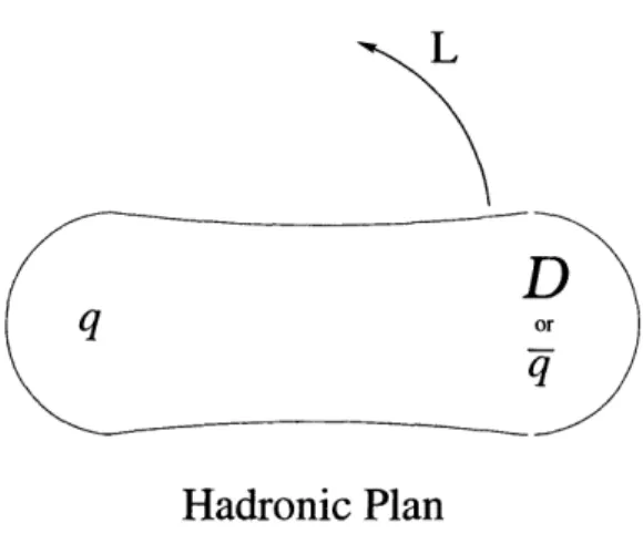
Contrarily the findings of Martin [29] show, under the context of potential theory, that the minimal energy state for baryons is a quark-diquark system and that their orbital angular momentum excitations lie on linear Regge trajectories with the same

L

Hadronic Plan

Figure 2-2: The typical rotating model for any hadron. Here "D" stands for diquark.

However, the most suggestive evidence for diquarks comes some from several

phe-nomenological indications. These include regularities in parton distribution functions,

and in the A fragmentation function [2, 27].

Finally because of their simplifying role, several phenomenalogical models have used diquarks. In particular, in the context of bag models, an obvious possibility is to model high angular momentum baryons as an extended flux tube with a diquark at one end and a quark on the other, as is done with mesons. Since 1975, Johnson and Thorn

[20] examined this possibility in a flux-tube type bag, which can be treated as a string

of constant tension whose value can be related to the fundamental bag parameters such as the "bag constant" B, and the strong coupling constant a,. Iwasaki et. al. [30, 31] undertook a similar program but postulating a "multibag" model where the diquark was placed into a separate internal bag (and the lone quark into it's own bag). As motivation for this, they separately calculate the masses of each bag, assuming little interaction between them, and then show that the masses of both separate bags sum to less than the one entire bag. The main difficulty with this reasoning,

however, is that they use energy terms from Ref. [12] that were derived with a color

confining boundary condition-a condition that is not realizable in a bag with a single quark/antiquark or diquark.

Nevertheless it is in the spirit of these phenomenological models, that we picture

thought as a spinning flux tube or string of constant tension T (remarkably despite what thickness it may have), and integer-quantized angular momentum. Although

such models were used in the past to explain general Regge-Trajectories observed in

the baryon sectors with some success, we show that by making some other simple assumptions, essentially all hadrons can be consistently well organized and explicitly

classified.

In particular the classification was first guided by considering several initial

hy-potheses motivated from arguments like those already discussed. After the classifica-tion was achieved, the hypotheses were confirmed and more generally modified, and new ones were also learned, in extraordinary consistency with a diquark interpreta-tion of baryons. I shall outline these final hypotheses in the next secinterpreta-tion. Explicitly, the initial hypotheses were (explanations to follow):

1. Baryons, at least with large total angular momentum L > 4 (quantized in integers), can be thought as being made of a diquark and quark in a rotating two body plan as described.

2. The dynamical two body model, implies that sets of resonances having the same internal quantum numbers (spins at the ends), lie along trajectories (Regge trajectories) of the form:

M

_{= a + L.}

_(2.2)

This is the well know Chew-Frautschi relation. Here M2 is the mass-squared of

the hadron (M will be used interchangeably with the energy E), is a slope

universal for all Regge trajectories, while a varies for each trajectory as defined

by the spins at the hadronic ends (including the distinction between good and bad diquarks).

3. The degrees of freedom at the end of the hadron are weakly coupled to each

other.

4. There is some expected difference in mass between a good and bad diquark. In

diquark as opposed to a good one.

2.3 Developed Hypotheses

All baryons were organized taking into account the "initial hypotheses". However as will be shown, upon classifying the hadrons, much was learned and the hypotheses

evolved into a more developed set that can exhibited in the data. These ideas are

summarized as the following "developed" hypotheses and are to be taken as what we

will conclude in this work:

1'. The diquark with quark model for baryons, in a two body or at least effective

two body plan, is valid down to L - 0.

2'. The Chew-Frautschi relationship extends down to L = 0. And so all baryons lie

on Regge trajectories, with a different for good and bad diquarks. The mesons

can also be shown to lie on similar trajectories, and there is a universal slope for both mesons and baryons.

3'. As we postulated originally, the degrees of freedom at the ends of the hadrons are indeed weakly coupled. However we shall find that for both small or large L, there may be overlap between wave functions. The only evidence of this is

manifested in the tunneling by a quark from a diquark to the other side. This

gives rise to a so-called "even-odd" effect exhibited only in certain symmetric cases where they should be. Thus we have a model where wave functions may

overlap, but dynamically and for purposes classification they behave as though

they do not, except for an expected and seen even-odd effect in some cases.

4'. Bad diquarks are clearly more massive than good diquarks. In E2 vs L space, this represents a larger a (Regge intercept) for bad diquarks. In general dif-ferent diquarks will imply difdif-ferent a values. From the semi-classical model of

the rotating baryons and by classifying and comparing mesons, we can extract

5'. A simple generalization of the Chew-Frautschi relation gives for heavy-light

quark/diquark systems:

(M _) 2 = a + 'L, (2.3)

2

where is the mass of the heavy end, and is the same universal slope.

6'. Spin interactions, besides those found internally within diquarks, are negligible.

2.4 Explanations of the Hypotheses

The two body plan in the first hypothesis was motivated for large L. We must simply let the experimental data dictate to us that it is universally valid for all L, or at least an effective two body plan is valid. It's validity is tested indirectly through the simple dynamical semi-classical model of the spinning flux-tube or string of constant tension T, since such a model implies the Chew-Frautschi relation. In what follows we will exhibit the general relation between the energy E and L, for spinning string of constant tension T and arbitrary masses at its end. When the masses are light, or the string rotates rapidly, the quoted Chew-Frautschi is reproduced perfectly. Specifically

the slope ao is related to the string tension by cr = 27rT. Hence because this is observed

at all L, we must assume that even for small angular momentum an effective two body system approximately holds.

Furthermore because the tension presumably arises from the color flux between the string/flux tube ends, a universal slope including those of the meson sectors implies that the same color charges reside in the baryon string ends, (i.e. the diquarks are there and they are anti-symmetric in color as discussed).

As will be shown, a pure string with massless ends leads to the relation E2 =

UL.

One might wonder what the proper interpretation of the observed Regge trajectory intercept, a, is. Strictly adhering to the classical string picture the only hope is to

make the ends of the strings massive. Of course, as is shown in the following section, this introduces some non-linearity in E2 vs L space for very small L, between 0 and

linearity between the ground state (defining the intercept) and L = 1, so that one would have to argue quite naturally that a breakdown of the simple string model with point masses might occur but conspires to keep things linear when matching L = 1 with 0. For one thing the mass distribution and short-range interaction between the ends should affect the model. In this interpretation, the existence and observed

differences in a could be explained quite naturally by differences in the non-negligible

effective masses for the different quarks and diquarks. The details of this possibility will further be discussed in the following section.

Finally, a second approach to explain the intercept, might posit the existence of some zero-point quantization effect in terms of angular momentum. Namely their might be some overall non-zero L manifest through the intercept. For example if

Lo = 0, goes to L' - Lo + a', the massless string trajectory is shifted to E2 =

aL + ua'. Variations in the actual a could then be explained again by variations in

quark/diquark masses, but requiring the actual values to be much smaller, thereby preserving the linearity of the Regge trajectory which is recovered perfectly in the

massless case.

The calculation for a string of the same tension but having one end very massive,

gives the relation between (E - )2, the mass of the particle without the heavy end,

squared, and L, as being linear with a slope 7rT, or half that of the slope for the light hadrons. This is seen experimentally for heavy-quark baryons, thereby implying the same universal tension for those as well.

Finally we note that the classification of the particles imply small spin-orbit forces. It has been suggested [2] that taking an interaction term as the fourth component

of a vector leads to a term of the form . L. But if one treats the potential as a

scalar, a similar term but opposite in sign results, thereby implying the potential to

be taken as vector° + scalar.

2.4.1

Generalization of the Chew-Frautschi Formula

We can generalize the Chew-Frautschi formula by considering two masses m1, m2

L. Our general solution will take a parameterized form in which the energy, E, and L are both expressed in terms of the angular velocity, w, of the rotating system. In the

limit that ml, m2 -- 0, the usual Chew-Frautschi relationship where E2 oc L can be

recovered. Other cases of interest in which analytic solutions of E2 vs L can be found

are those when one mass is infinitely heavy and the other is approximately zero, or when both are infinitely heavy.

One can begin by considering the masses ml and m2 distances rl and r2 away

from the center of rotation respectively. As implied, the whole system spins with angular velocity w. It is also useful to define in the usual manner:

,'i /1 1 (2.4)

where the subscript i can be or 2 (for the mentioned masses). Then it is straight-forward to write the energy of the system:

T

T

E

+-

w J0 x/1-u 220

J

The last two terms are associated with the energy of the string. Similarly the angular

momentum can be written as:

T w u T w 2 2

2 2~~~~~r 2fr

L m

wr2

-mwr2

+

+

/1

du -

o

du. (2.6)

Carrying out the integrals gives: T

E =- rl/yl1 + m2Y2+ -(arcsin[wrl] + arcsin[w)r2]), (2.7a)

W2 2

L =

±

1

(-wrl/1- (wrl)

_±

_arcsin[r

l

]

/1

)

+ arcsin[r

])

Furthermore for each mass, the following relationship between the tension and angular acceleration must hold:

mi 2ri =

T.

(2.8)

We can use this to do away with the distances rl and r2 and express everything in

terms of w. Specifically we note that in our expressions for E and L, the quantities

that contain ri, are -yi and also wri. From equation 2.8 we can ultimately solve for 7i:

i =

|1 A/l

+ 4(T/(miwv))2(29

And finally from equation 2.8 we also know that wri is just T/(mi-i2w).

We are now in a position to replace these terms in equation 2.7 and write E and

L in terms of the parameter w and other quantities known by definition, namely the

masses and the string tension T. To this effect, perhaps the most useful way to write

the expressions is to define another variable xi m which can later serve as an

expansion parameter for small masses mi (or large L). Making replacements into

equation 2.7 we obtain:

E

Zmi

±+ ±i/ + -arcsin

1

(2.1Oa)

X/

+

x/4)

L T 1

rx

i

X

-

-- aci[/2

(2.10b)

i=1,2

(+1

While it may difficult to gain insight from these expressions, we can actually make

much use of them by either parametrically plotting £2 vs L (C-F plot) for whatever

values of inl, in₂, and T desired, or if we are considering either very light or very

heavy masses, appropriate expansions can be made to obtain analytic expressions for_{£E~x2 L.- vs}

With regard to making appropriate expansions, it is important to note that the

terms associated with each mass are completely decoupled from each other, as the_{Xi=12 1Xi} q _2/ - ₂

Xi 2 q- xi~~~~~~~~~~X

vaue o m, 2,an Tdeired, _{or if we~ ar cosidrng either veylgt.rvr}

E ~~~~~~~2 1sL

Wieith reayrdicl to main isgh aproprite expresions, it isiprantont atual mte

expressions involve just a sum of contributions from each mass. Hence, one can make

expansions for any given mass up to the necessary order, or with whatever parameter (depending on whether the mass is very heavy or very light, where this approach makes sense). In light of this it is reasonable to talk about the contribution of a single mass to E or L without regard for the other. Hence we'll adopt a convention

that denotes the contribution from one mass by a , as in E in what follows. In particular if a given mass mi is very light or for large L, then as suggested xi serves as a good expansion parameter. If we expand in xi, then, we find the contribution to

the energy,

6E,

be (carried out to order x 5/2):

- ~~~~~( 7rT 1 W112 M3/2 1 5/2 _3/2 3 m5/2 7/2 7/2) fight-- 2( 3 - i 2 20 T 224 T (2.11a)

L

±0

For a system with two light and equal masses, we would of course just multiply the right hand side of these expressions by two to obtain the total energy and angular

momentum. Also note that at least for a very light mass it seems that as L - 0,

w - oc and taking this limiting case in the general expressions shows that this is

indeed the case. As such, care must be taken to make sure that the expansions are

valid depending on L values. In practice therefore it is much more useful to look at parametric plots at least as a check. However, if we let both masses go to zero,

and therefore take only the first term for each mass from the light-mass expansion (equation 2.11), then the we recover the familiar Chew-Frautschi relationship for the string with massless ends:

E2= (2rT)L. (2.12)

Of course, a different regime is that where one or both masses become infinitely

heavy. In this case, we might instead expand terms for a given mass with a parameter

_ T . As before we can expand the contribution from one mass, but this time a

heavy one, as follows (expanded to 4th order in 1xi):

3 T2 35 T4 _mj

Eheavy = mi 2 m 2 24 3 4 + (2.13a)

6Lheavy- miW3 . w3 + °(2 5 (2.13b)

'MiW 3 6 i_i 503 2xi

Using these expansions one can easily find the analytic solution for the case of one

very heavy mass M connected to a light mass (approximately zero). Specifically for the heavy mass contribution we can take just the first term for the energy and none for the angular momentum from equation 2.13; and the first terms of equation 2.11 for the contributions of the light mass. This would give the expressions:

E = M + 2rT _{E=M+ 2w} (2.14a)

irT

L = 4w2' (2.14b)

which ultimately yields the relationship:

(E - M)2 =

wTL.

(2.15)

Hence we see that the C-F relationship for a heavy-light mass system is the same as the two-light-masses case but with half the slope and with the energy shifted by that of the heavy mass.

In reality, however, many interesting examples fall between these mentioned lim-iting cases. As already suggested, to see the behavior of all these other cases, we

must simply examine parametric plots of expression 2.10. Doing so one finds that for a robust range of masses, the extremal cases are well approximated. Several of these

Chapter 3

The Classification of Particles

3.1 Methods

In practice, classifying the particles involves first listing the possible diquark-quark states and searching out candidates based on their energies, total angular momentum, and parity. For sectors containing few particles, this program is not very difficult. However, the formidable nucleon-delta complex with its plethora of particles may

present an interpretive challenge. To handle such a case, and in the future as more

particles are discovered, I will outline a visual and intuitive method to aid in the

classification.

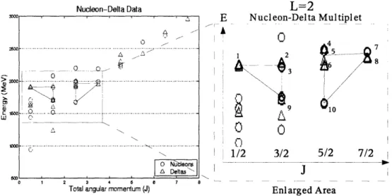
To classify the particles "visually", one should plot the particles from a given

complex in E vs L (J, total angular momentum also implied), differentiating between particles and their parity. Figure 3-1 (on the left) shows this for the nucleon-delta complex. Note, that only resonances having 2* or better rating according to the Particle Data Group (PDG) [32] are plotted and considered throughout this work. The goal is then to establish what I shall call the "constant-L" diagram for the sector. As the name suggests this is a diagram which groups all particles with a given angular momentum in E vs L space. The diagram will have some approximate geometric shape whose vertices are the corresponding particles for that given L. Thus the classification then becomes a simple matter of visually identifying this shape in the plot containing all particles.

Nucleon-Delta Data

0 1 2 3 4 5 a

Tolal angular momentum (J)

L=2 E Nucleon-Delta Multiplet 0 A2 JA 1

, L

9

Figure 3-1: Multiplet of nucleon-deltas with L = 2, as taken from the data plotted on the left. In practice the particles are easily grouped based on parity. The numbered

particles identified as L = 2 on the right correspond to 1 A(1910), 2 A(1920), 3 N(1900), 4 A(2000), 5 N(2000), 6 A(1905), 7 N(1990), 8 A(1950), 9 N(1720), 10

N(1680).

E

(ud)--u ord

-[ud]--u ,ord

-Constant-L Diagram Construction

For Nucleon-Delta Sector

2 L-3/2 L-i/2 L-/2LL L 1/2 L+3/2 i Nucleons O Nucleons J A Deltas

Figure 3-2: Shown here is the expected multiplet of nucleons and deltas for a given

value of L plotted linearly in energy versus total angular momentum. The diagram can be constructed first by considering the possible quark contents and noting the hypothetical separation in their energies, thus creating the two rows as well as deter-mining what particles are allowed in each row. Finally for a given quark content, the different allowed spin configurations are considered. Note that depending on the spin

interactions, the rows may have a slope as shown. Also note that a different diagram is to be expected for every sector.

2500 2000 MO0 a 0 W 4 A ~~o /. , . . ... ... ... .. ... ... ... ... ... . ... ... .. . .. ... . ... )...I... ... ... ... ... .. 0 Nleor , , O ,_ I 7 10oo l l 2 R W v I \, i i I :F A -1 --- l I I

To find the diagram, which will be different for every sector, we first label on the

energy axis the diquark-quark combinations that are possible in that sector. Here one must make a prediction between the relative energy difference between the diquarks.

The idea is just to postulate some ordering and energetic spacing between the different diquark-quark constituents in the sector. For the nucleon-delta sector this is shown in Figure 3.2. Next, one labels the center L for the graph and considers the different spin states that the quarks and diquarks may take and whether they are aligned or not. In the limit of no spin-dependent forces, the particles with different spins are all

equivalent in energy and should therefore lie on a horizontal line from the energy of

its respective diquark. For greater spin forces, the lines for increasing total L should be upward sloping. Again the example for the nucleon-delta sector is shown. Note the manifestation of hypothesis 6': that the spin-dependent forces outside of diquarks are indeed feeble. Also note that these considerations determine not only the possible shape, but what particles can be found where. In this example the good diquarks can

only have total L of only L ± 2:

1 1

L X 2 =(L+ )(L- (3.1)(3.1)

2 2 2

Bad diquark-containing particles, contain particles from L - ₂₂to L + :

1 3 1 1 1 1 3

L 1

-=(L+ )D(L + ®)D(L+ ®(L- 1)®(L- )®(L- ) (3.2)

(with of course the understanding that negative values are to be dropped).

Further-more in terms of isospin, the bad diquark has isospin 1 (flavor symmetric, as discussed

above), which can be paired with the isospin quark to give both nucleons and deltas essentially degenerate.

Once this multiplet with the same L can be identified, then it can be matched to

the particles in the whole plot, which in practice can easily be done by identifying

particles of the same parity as shown in Figure 3-1. Also the center of the multiplets should rise for the different L, according to E oc v/.

unnecessary given the sparseness of the present data, however, it provides a good

template for classifying future discoveries. Also, we must not forget that while

classi-fying the particles in this way may help distinguish between possible ambiguities, for the purposes of the following analysis we are actually not interested in particles of the same angular momentum, but in the set of different angular momenta for particles having the same quantum numbers (i.e. the Regge trajectories). These sets can then

be plotted in in E2 vs L and fitted according to the Chew-Frautschi relationship.

What follows presents the classification of all baryons established by the PDG [32]

with 2* or better, and all mesons marked by a dot ().

3.2 The Light Baryons

3.2.1

Nucleon-Delta Complex

The classification of essentially all nucleon-delta particles are shown in Table 3.1.

This table and all others from here on are divided into series, designated by Roman numerals, representing the different possible net spin alignments. These are further divided into the possible ways of obtaining the net spin alignment, and they are denoted by letters. Furthermore we adopt the graphical convention of a simple dash

(-) for a spin singlet and a double arrow for a vector diquark (such as or ).

Arrows pointing up are aligned, and down anti-aligned. Also we generically label an isospin quark (u or d) simply as 1, unless they are found paired as a good diquark in

which case they are explicitly written, [ud], and understood to be antisymmetric. The first series assumes maximal alignment between orbital and spin angular momentum. For L = 0 there is a unique nucleon state, since (assuming spatial symmetry) spin

symmetry and color antisymmetry imply flavor symmetry. For larger values of L

there is both a good diquark and a bad diquark nucleon state. The latter is made

by assembling the I = 1 bad diquark with the I = 1 quark to make 2

According to hypothesis 3', independence of the two ends, we should expect to have approximately degenerate bad diquark nucleons and deltas. Examples of this include

Table 3.1:

Nucleon-Delta Classifications.

I.

Angular

A. [ud]-

1

B. (ud)-

1

Momentum (L) - T

f

0

N(939) 1/2

A(1232) 3/2

1

N(1520) 3/2-

N(1675)

5/2-2

N(1680) 5/2

_{A(1950) 7/2}

_{N(1990) 7/2}

3

A(2400) 9/2-

N(2250)

9/2-4

N(2220) 9/2

A(2420) 11/2

5

N(2600) 11/2-

A (2750)

13/2-6

N(2700) 13/2

A(2950) 15/2

I.

A. [ud]-1

B. (ud)-1

Angular

-

I

1

N(1535) 1/2-

A(1700) 3/2-

N(1700)

3/2-2

N(1720) 3/2

_A(1905)

_5/2

_{N(2000) 5/2}

3

N(2190) 7/2

4

A(2300) 9/2

Im. Two "units" less then maximal alignment.

A. (ud)- 1

4

T

:-l-1

A(1620) 1/2-

N(1650)

1/2-2

A(1920) 3/2

N(1900) 3/2

3

N(2200)

5/2-IV. Maximal "bad" diquark anti-alignment.

Angular

A. (ud)-1

Momentum (L)

. 4

2

A(1910) 1/2

3/2-the A(1950) 7+ with the N(1990) 7+ in the first series, the A\(1920) 3+ with the

N(1900) ₂+ in the third series, and some other more corrupted pairs. In general,

the existence of a second nucleon series corresponding to a bad diquark is direct

implication of this diquark model with weakly coupled degrees of freedom, rather

than one whole antisymmetric nucleon ground state. Furthermore there seems to be a clear energetic distinction between good and bad diquarks of about 200 MeV as can be seen by comparing the first and third columns of the series.

Classifying the particles in this manner also shows that their are particles yet to be discovered. In particular the predictions can be made for the existence in the first

series of a N(2000) and a A(1700) . Also the Z(2400) is relatively high in

mass and thus we would expect it to be about 100 MeV lighter.

The second series includes cases where the spin and orbital angular momenta sum up to one less than the maximum possible J. We do not expect any states for L = 0 since with no separation of the two ends, the bad diquark formation is

unfavored. Note that in that in the second two columns of this series there are two

possible spin alignments (see the decomposition in the 3rd paragraph of the "methods" subsection). Thus there should be a degenerate state for particles here. Only one

possible candidate pair is found: the A(1905) + (2000) and 5+, of which we predict

that the A(1905) is too low.

Finally recall as previously mentioned the feebleness of spin forces, most

am-ply seen at the L = 2. We find two nearly degenerate good-diquark nucleons

N(1680),N(1720) with JP - 5+ 3+; and a host of nearly degenerate bad-diquark

nucleons and deltas N(1990) 7+, N(2000) 5+' N(1900) 3+, A(1950) 5+, A(1905) 5+,

A(2000) 5+' A(1920) 3+' (1910) +.

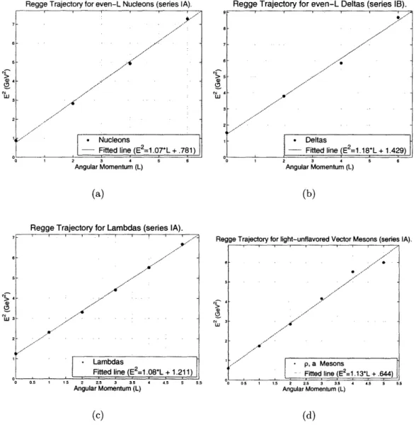
We now begin to consider the evidence for the Regge Trajectories implied in hypotheses 1 and 2. In particular, series IA and the deltas of IB, are most represented. However, upon plotting these, we find a most consistent pattern: that the odd-L particle have more energy than their even-L partners. This so called "even-odd" effect

is shown explicitly in Figure 3.3. A possible explanation for this effect might be that

All Nucleons of series IA.

Angular Momentum (L)

(a)

LU

w

Even-L Nucleons of Series IA.

7 4 . 2 ₃₁ - _. s/ i i,"' 0 1 2 3 4 5 Anaular Momentum (L) (b)

Figure 3-3: (a) Plot of nucleons showing "even-odd effect". (b) Just the even-L where

the trajectory is truly linear. Dashed line shown for reference.

Figure 3-4: Symmetric hadron with tunneling quark to produce the same baryon

rotated by 7r. IF qq q) x10 4 w c i i I i~~~~~~ - . . - .. . ... .I 1. -0 F 1 0

for certain symmetric cases such as in the nucleon-delta sector such a tunneling would amount to a rotation of a fixed bone through r as shown in Figure 3.4. Therefore we

should construct spatial wave functions that are symmetric or anti-symmetric under

this exchange. The symmetric case, would be node-less and therefore have less energy,

while the opposite is true for the antisymmetric case. The even L would correspond to the symmetric case while the odd L to the antisymmetric one. Hence we should expect that when tunneling of this kind is significant, there be some separation between the even and odd L. We can say something more quantitative about this effect, but will relegate that discussion to its own section following the classification of the other baryons.

When the even-odd effect is accounted for by separating out the series into even and odd L, the trajectories are very linear as predicted. Table 3.2 shows the observed values for all classified series. Note that many series are sparse and contain just two

points which trivially make a line and gives a poor estimate for the universal slope.

Nevertheless many of these are still in surprising agreement. If we consider the most prominent trajectories, the picture is even more consistent. The values for these are

isolated in Table 3.3. We find an average slope from these of 1.18 GeV2. Finally plots for the more prominent fits of all the classifications are shown in Figure 3.5 and should serve the reader as a reference in the following sections.

3.2.2

Other Light Baryons

Tables 3.4 and 3.5 show the bulk of our classifications for all other light hadrons (no nucleon-deltas). First we consider the lambda-sigma sector or baryons containing two light one strange quark (lls). Four possible diquark configurations come into play:

[ud], (11), [Is], (s). Since the [ud] diquark is so favorable we would expect it to be well represented, and indeed we find a very clear trajectory from L = 0 to L = 5

of A baryons in the first series. In this trajectory we predict that the spin-parity of

A(2350), which is debated, should be _2' 9+ , while that of A(2585) should be 11 ₂ . In

general all particle classified with unknown spin-parity may be regarded as predictions

Table 3.2: Listed here are all the fitted slopes and intercepts for all series correspond-ing to light hadrons; includcorrespond-ing those with two just points. Note that even many of these are quite consistent in their slope! "Sector" refers to the hadron type which can

be found in tables 3.1 to 3.7. "Series" corresponds to the different Regge trajectories

as labeled in the respective tables. The parameters correspond to a fit of the relation

E2 L + a.

points

Sector Series in series a (GeV2) a (GeV2)

nucleons IA. even 4 1.07 .781

nucleons IA. odd 2 1.112 1.198

nucleons IB. odd 2 1.128 1.677

nucleons IIB. odd 2 .953 1.937

nucleons IIIA. odd 2 1.059 1.664

deltas IB. even 4 1.18 1.429

deltas IB. odd 2 .901 3.056

deltas IIB. odd 2 .738 2.339

lambdas IA. 6 1.08 1.211

sigmas IB. even 3 1.15 1.404

sigmas IB. odd 3 1.09 1.849

sigmas IC. even 2 1.101 1.919

cascades IA. even 3 .969 1.779

rho/a IA. 6 1.13 .6444 rho/a IIIA. 2 .788 1.325 omega/f lB. 5 1.16 .5527 omega/f IIIB. 3 1.082 .7166 phi/f IC. 3 1.19 1.072 phi/f IIIC. 2 1.35 1.09

pi/b IIa singlet 3 1.385 .0599

eta IIbA singlet 3 1.20 .2574

eta' IIbB singlet 2 .983 .9216

kaon I. 5 1.19 .7962

kaon II. 5 1.56 .229

Regge Trajectory for even-L Deltas (series B). cai w > Angular Momentum (L) (a)

Regge Trajectory for Lambdas (series IA).

// 4 r/" 2 ;... -- | *Lambdas Fitted lne (E2=1.08*L + 1.211) 0.5 1 I 5 2 2.5 3 3.5 4 4.5 5 Angular Momentum (L) (c) Angular Momentum (L) (b)

Regge Trajectory for light-unflavored Vector Mesons (series IA).

%wo

0 OA 1 1.5 2 2.5 3 3. 5

Angular Momentum (L)

(d)

Figure 3-5: Plots of the most prominent Regge trajectories. 423 > %j ID > %J Nt2. S -~~~~ ,7 , * , 3 . . . v · . 2 ~ ~~~~~~~~~~~~~~/.. ,.//' '7v./ .-,|*p, " a Mesons ..|--Fitted line (E2=1.13*L + .644) O. ,.

Regge Trajectory for even-L Nucleons series IA).

Table 3.3: These are the fitted parameters as before, but only with series containing

three or more points. The average based on these is 1.18 GeV2, with standard deviation .149.

points

Sector Series in series a (GeV2) a (GeV2)

nucleons IA. even 4 1.07 .781

deltas IB. even 4 1.18 1.429

lambdas IA. 6 1.08 1.211

sigmas IB. even 3 1.15 1.404

sigmas IB. odd 3 1.09 1.849

cascades IA. even 3 .969 1.779

rho/a IA. 6 1.13 .6444

omega/f IB. 5 1.16 .5527

phi/f IC. 3 1.19 1.072

pi/b IIa singlet 3 1.39 .0599

eta Ib singlet 3 1.20 .2574

kaon I. 5 1.19 .7962

kaon II. 5 1.56 .229

particularly striking, and no even-odd effect is discernible in it. This is consistent with our tunneling interpretation, since for [ud]s rotation through r can only be mimicked

by triple-tunneling, which plausibly is negligible.

With these classifications in place, we might expect to find a more energetic trajec-tory of sigmas containing a [Is] diquark and an approximately degenerate trajectrajec-tory

of lambdas (with the right combination of isospin, 3 0). Experimentally, while

the lambdas are not [yet] seen, there is a plausible sigma trajectory, which implies a

splitting of [Is]- [ud] -. 100 MeV. Presumably an (11) diquark assignment to these

would produce a higher splitting, allowing us to conclude this to be the correct clas-sification. Furthermore, according to our even-odd effect hypothesis, such a series contains favorable tunneling conditions to produce such an effect. On a typical Regge plot, it becomes difficult to see the effect, but it certainly exists on a much smaller scale. This would indicate the tunneling amplitude here is much smaller than the purely light quark case of the nucleon-delta sector. We can see a clear signature for

the effect by searching for oscillating slopes between particles of even-L and odd-L. Doing this for the slopes between L = 0 and 1, 1 and 2, 2 and 3, etc., we find values

Table 3.4:

Lambda-Sigma Classifications

I.

IIa.

One "unit"

and "bad" diquarks.

less than maximal alignment.

A. [ud]- s

B. [ls]-1

C. (ls)-l

Angular

-

L

-

t ,

_

Momentum (L) or =-T

1 A(1405) 1/2- E(1620) 1/2- A(1670) 1/2- NONE

2(1690) 7?

2 A(1890) 3/2+

IIb.

One "unit" less than

Angular

A. ud

-s

B. [ls]-

C. (s)-

.

Mom.

(L)

--

I

--

t

'

t

0 A(1116) 1/2+ 2(1193) 1/2+ Z(1385) 3/2+

1 A(1520) 3/2- Z(1670) 3/2- A(1690) 3/2- E(1775) 5/2- A(1830)

5/2-2 A(1820) 5/2+ Z(1915) 5/2+ Z(2030) 7/2+ 3 A(2100) 7/2- Z(2250) ?? 4 A(2350) 9/2+ 2(2455) ?? 5 A(2585) ?? 2(2620) ??

A. s)-1

.

of 1.36, .878, 1.39, .964, and .837 GeV2 respectively, all of which, with the exception

of the last one follow the desired pattern. As such we predict that mass estimates for the the E(2620) (the last resonance of this series) are too low should it be found

with JP = 11. ₂ As a check, undertaking the same analysis between all points in the

A series IA, we find a completely constant slope as expected.

Finally we examine the bad diquark members of this series (with (11)), expecting both lambdas and sigmas depending on their isospin. There are three appropriate E

candidates for L = 0,1, 2 and one A for L = 1 (note that the A configuration is

for-bidden by Fermi statistics for L = 0, assuming a common spatial wave function). The Es could support either () or (s) diquarks; the observed eigenstates are presumably

a mixture. The A(1830) is fully 55 MeV heavier than its E(1775) "partner",

and 310 MeV heavier than the good-diquark A(1520) 3-. ₂ These splittings are a bit

larger than others of the same kind we see elsewhere. As expected, there is also an indication of an even-odd effect here. Indeed, (13852 + 20302) = 1738 < 1775. Also looking the slope between E(1385) and E(1775) we find a value of 1.23 GeV2, while between E(1775) and E(2030) a lower one of .97 GeV2 as expected.

The second and third series are more sparsely represented (the fourth is not even

seen), and they present some challenging puzzles. The A(1405) i surprisingly

light and it has been suggested that its mass may be perturbed by the nearby NK

threshold [2]. Also the absence of a good candidate for the A state corresponding to good-diquark [ud]s for L = 2, while [us]d has one, is also surprising. Finally there are

two 2* E resonances in the mass region where we expect the L = 1, JP = 1, namely

A(1620) - and A(1690) ??. Ideally these should be represented as the same state with some intermediate mass [2]. Finally, the complete absence of representatives of the bad diquark configurations (s)l in the second series, while appearing in the first

series and third, lead one to predict the existence of E(1760) , E(2055) -, A(1815)

to fill in the holes. (All these masses should be taken ±50 MeV.) [2]

Nevertheless, in good agreement with hypothesis 6' we have approximate

degenera-cies: (1670) , A(1690) -, A(1670) -, (1620-1690?) ; E(1915) 5+, A(1890)

-Table 3.5:

Cascades and Omega Classifications

I.

Angular

A.

s

-s

B.

s

s C.

s)

s

I

i

I

0

-(1318) 1/2

_{(1530) 3/2}

_{Q(1672) 3/2}

II.

A. (ls)-s

Angular _f-l

Momentum (L) or X T

1

E(1820)

3/2-2 E(2030) ??

as seen in Table 3.2, the slopes are consistent with the universal value.

The data on cascades is also sparse, especially in regard to spin-parity assign-ments, so that the classification are necessarily assumptive (see Table 3.5). Should these correct assignments, then it is noteworthy to mention that here too one finds

os-cillating slopes, especially in series IA, as expected from the tunneling of the quark. We also find a lower than usual slope between E(1820) and E(2030)-all in agreement

with the even-odd effect. The omega sector data is worse, to the point where nothing interesting can be said.

3.3 The Light Mesons

The classification of the mesons do not require any novel ideas with regard to the pre-vious literature-there are no diquarks, and the string model is as old as the field itself. Nevertheless drawing the analogy of the mesons to the diquark model of baryons, it is

Table 3.6:

Light Unflavored

I.

Angular

All with spin

Momentum

(L)

A.

=

B. I

=

0, no

sS

C.

S

0

p(770) 1--

w(783) 1--

q(1020)

2

p(1690) 3--

w(1670) 3--

q(1850)

4

p(2350)

IIa.

I

Angular

spin triplet

spin singlet

Momentum (L)

-0 7r(140) 0- +

1 a(1260) 1+ + _{b(1235) 1}+

-2 7r(1670) 2 +

ib.

Angular

A.

with no s

B.

s-Momentum (L)

0

/(550) 0

r'(960) 0

1 f(1285) 1+ + _{(1170) 1}+ - _{f(1420) 1}+ + _{I'(1380) 1}+

-2

r/(1645)

III. Maximal spin anti-alignment

Angular

All with spin

4

Momentum (L)

A. I

=

1 B. I

=

0,

with no

s

C.

SS

1 a(1450) 0+ + f(1370) 0+ + f(1500) 0+ +

2

p(1700) 1--

w(1650) 1--

0(1680)

1--3 f(2010) 2+ + f(2300) 2+ +

Table 3.7:

Light Strange Mesons (S

1)

Angular I. Spin aligned II. Spin neutral III. Spin anti-aligned

Mom. (L) 1' X or- 4 0 K*(892) 1- K(495) 0-1 K*(1430) 2+ K(1270) 1+ K(1400) 1+ K*(1430) 0+ 2 K*(1780) 3- K(1770) 2- K(1820) 2- K*(1680) 1-3 K*(2045) 4+ K(2320) 3+ 4 K*(2380) 5- K(2500)

4-instructive to classify and fit the meson series to Regge trajectories to compare their slopes and for possible calculations in comparing quark masses to diquarks masses.

As such, our classification of the light mesons (those classified with a dot in the PDG) are listed in Tables 3.6 and 3.7, while their Regge fit values are given in Table 3.2.

In particular this program yields consistent slopes with the baryons, supporting the idea of the diquark as effectively having the color of an antiquark. There are also approximate degeneracies for states with the same L but different spin alignment, and in several cases we have approximately degenerate particles corresponding to a vector meson neutrally aligned versus a singlet.

The i7r(140) is not surprisingly a little anomalous, and it causes the trajectory to have a small intercept and higher than usual slope (entry pi/b in Table 3.2). However this L = 0 may well be described in another language, as an approximate

Nambu-Goldstone boson [2].

3.4 Exceptional Cases

There were several particles that were not classified. In the traditional quark model these all correspond to being interpreted as having internally excited quarks or in some cases the particles defy classification. The diquark system presents no inconsistencies with any of the traditional views. It does, however, offer the possibility of some new interpretations. Nevertheless, to give a better treatment of these ideas, it is necessary to have a better understanding of effective diquark masses and mass parameters