Learning to Survive: Achieving Energy Neutrality in Wireless Sensor Networks Using Reinforcement Learning

HAL Id: hal-01530098

https://hal.archives-ouvertes.fr/hal-01530098

Submitted on 31 May 2017

HAL is a multi-disciplinary open access

archive for the deposit and dissemination of

sci-entific research documents, whether they are

pub-lished or not. The documents may come from

teaching and research institutions in France or

abroad, or from public or private research centers.

L’archive ouverte pluridisciplinaire HAL, est

destinée au dépôt et à la diffusion de documents

scientifiques de niveau recherche, publiés ou non,

émanant des établissements d’enseignement et de

recherche français ou étrangers, des laboratoires

publics ou privés.

Learning to Survive: Achieving Energy Neutrality in

Wireless Sensor Networks Using Reinforcement Learning

Fayçal Ait Aoudia, Matthieu Gautier, Olivier Berder

To cite this version:

Fayçal Ait Aoudia, Matthieu Gautier, Olivier Berder. Learning to Survive: Achieving Energy

Neu-trality in Wireless Sensor Networks Using Reinforcement Learning. IEEE International Conference

on Communications (ICC), May 2017, Paris, France. �hal-01530098�

Learning to Survive: Achieving Energy Neutrality in

Wireless Sensor Networks Using Reinforcement

Learning

Fayçal Ait Aoudia, Matthieu Gautier, Olivier Berder

University of Rennes 1, IRISA

Email: {faycal.ait-aoudia, matthieu.gautier, olivier.berder}@irisa.fr

Abstract—Energy harvesting is a promising approach to enable autonomous long-life wireless sensor networks. As typ-ical energy sources present time-varying behavior, each node embeds an energy manager, which dynamically adapts the power consumption of the node to maximize the quality of service, while preventing power failure. In this work, RLMan, a novel energy management scheme based on reinforcement learning theory, is proposed. RLMan dynamically adapts its policy to time-varying environment by continuously exploring, while exploiting the current knowledge to improve the quality of service. The proposed energy management scheme has a very low memory footprint, and requires very few computational power, which makes it suitable for online execution on sensor nodes. Moreover, it only necessitates the state of charge of the energy storage device as an input, and therefore is practical to implement. RLMan was compared to three state-of-the-art energy management schemes, using simulations and energy traces from real measurements. Results show that using RLMan can enable almost 70 % gains regarding the average throughput.

I. INTRODUCTION

Many applications, such as smart cities, precision agri-culture and plant monitoring, rely on the deployment of a large number of individual sensors forming Wireless Sensor Networks (WSNs). These individual nodes must be able to operate for long period of time, up to several years or decades, while being highly autonomous to reduce maintenance costs. As refilling the batteries of each device can be expensive or impossible if the network is dense or if the nodes are deployed in a harsh environment, maximizing the lifetime of typical sensors powered by individual batteries of limited capacity is a perennial issue. A more promising solution is to enable the nodes to harvest the energy they need directly in their environment, by equipping them with individual energy harvesters.

Various sources can be considered to power the nodes, such as light, wind, heat or motion [1], [2]. However, because most of these sources present time-varying behavior, the nodes need to be able to dynamically adapt their performance to fully exploit the harvested energy while avoiding power failure. Therefore, for each node, an Energy Manager (EM) is respon-sible for maintaining the node in Energy Neutral Operation (ENO) [3] state, i.e. the amount of consumed energy never exceeds the amount of harvested energy over a long period of time. Ideally, the amount of harvested energy equals the amount of consumed energy over a long period of time, which means that no energy is wasted by saturation of the energy storage device.

Many energy management schemes were proposed in the last years to address the non trivial challenge of designing effi-cient adaptation algorithms, suitable for the limited resources provided by sensor nodes in terms of memory, computation power, and energy storage. The first EM scheme was intro-duced by Kansal et al. [3] in 2007. Their approach relies on an energy predictor, which estimates the future amount of harvested energy. In [4], Vigorito et al. introduced LQ-Tracker, an EM that uses Linear Quadratic Tracking to adapt the duty-cycle by considering only the state of charge of the energy storage device. Another approach proposed by [5] and [6] is to use two distinct energy management strategies, one for periods during which harvested energy is available, and one for periods during which the harvested energy is below a fixed threshold. More recently, Hsu et al. [7] considered energy harvesting WSNs with throughput requirement, and used Q-Learning, a well-known Reinforcement Learning (RL) algorithm, to meet the throughput constraints. The proposed EM requires the tracking of the harvested energy and the energy consumed by the node in addition to the state of charge, and uses look-up tables, which incurs significant memory footprint. In [8], Peng et al. formulated the average duty-cycle maximization problem as a non-linear programming problem. As solving this kind of optimization problem is computationally intense, they introduced a set of budget assigning principles, which forms P-FREEN, the EM they proposed. With GRAPMAN [9], an EM scheme which focuses on minimizing the throughput variance, while avoiding power failure, was proposed. In [10] the authors proposed with Fuzzyman to use fuzzy control theory to dynamically adjust the energy consumption of the nodes.

Most of these previous works require an accurate control of the spent energy and detailed harvested and consumed energy tracking to operate properly. However, in practice, such mechanisms are difficult to implement and incur significant overhead [1]. Considering these practical issues, we propose in this work RLMan, a novel EM scheme, based on RL theory, that requires only the state of charge of the energy storage device to operate. RLMan aims to maximize the quality of service, defined in this work as the throughput, i.e. the frequency at which packets are sent, while avoiding power failure. RLMan aims to find a good policy for setting the throughput, by both exploiting the current knowledge of the environment and exploring it to improve the policy. The major contributions of this paper are:

‚ A formulation of the problem of maximizing the quality of service in energy harvesting WSNs using the RL framework.

‚ A novel EM scheme based on RL theory named RLMan, which requires only the state of charge of the energy storage device, and which uses function approximation to minimize the memory footprint and computational overhead.

‚ The evaluation of RLMan as well as three state-of-the-art EMs (P-FREEN, Fuzzyman and LQ-Tracker) that aim to maximize the quality of service, using extensive simulations with real measurements of both indoor light and outdoor wind.

The rest of this paper is organized as follows: In Section II, the problem of maximizing the throughput in energy harvesting WSNs is formulated using the RL framework, and Section III presents the derivation of RLMan based on this formulation. In Section IV, RLMan is evaluated. First, preliminary results are presented to show the behavior of RLMan, focusing on the learning phase (first few days). Next, the results of the comparison of RLMan with three other EMs are exposed. Finally, Section V concludes this paper.

II. FORMULATION OF THEENERGYHARVESTING PROBLEM

It is assumed that time is divided into equal length time slots of duration T , and that the EM is executed at the beginning of every time slot. The amount of residual energy, i.e. the amount of energy stored in the energy storage device, is denoted by eR and the energy storage device is assumed to

have a finite capacity denoted by E_Rmax. The hardware failure threshold, i.e. the minimum amount of residual energy required for the node to operate, is denoted by E_Rmin. It is assumed that the job of the node is to periodically send a packet at a throughput denoted by f P rFmin_{, F}max

s, and that the goal of the EM is to dynamically adjust the performance of the node by setting f . The goal of the EM is to maximize the throughput f while keeping the node sustainable, i.e. avoiding power failure. In the rest of this paper, a "t" subscript is used to denote values associated to the tthtime slot.

In RL, it is assumed that all goals can be described by the maximization of expected cumulative reward, where a reward denoted by R is a scalar feedback describing how well the node is performing. Formally, the problem is formulated by a Markovian Decision Process (MDP) xS, A, T , R, γy [11], described in detail thereafter.

The set of states S: The state of a node at time slot t is denoted by St and is defined by the current residual energy

eR. Therefore, S “ rERmin, E max R s.

The set of actionsA: At each time step, an action, denoted by At, is taken, which corresponds to setting the throughput

f at which packets are sent. Therefore, A “ rFmin_{, F}max

s. The transition functionT : The transition function gives the probability of a transition to e1

Rwhen action f is performed in

state eR. Because the state space is continuous, the transition

function is a probability density function such that: ż

E1 R

T peR, f, e1Rqde1R

“ Pr“St`1P ER1 | St“ eR, At“ f‰ . (1)

The reward function R: In this work, the reward is computed as a function of both f and eR:

R “ φf, (2)

where φ is the feature, which corresponds to the normalized residual energy:

φ “ eR´ E

min R

E_Rmax´ E_Rmin. (3) Therefore, maximizing the reward involves maximizing both the throughput and the state of charge of the energy storage device. However, because the residual energy depends on the consumed energy and the harvested energy, and as these variables are stochastic, the reward function is defined by:

Rf

eR“ E rRt| St“ eR, At“ f s . (4)

The discount factorγ: The discount factor takes values in r0, 1s. Its function will be explained below.

The transition function T describes the dynamics of the environment and is assumed to be unknown. Similarly, if the reward is computed using (2), its value is actually stochastic as it depends on the residual energy. The behavior of a node is defined by a policy π, which is a conditional distribution of actions given states:

πpf |eRq “ Pr rAt“ f | St“ eRs . (5)

The objective function J is defined as the expected sum of discounted rewards regarding a policy π and an initial state distribution ρ0: J pπq “ E «₈ ÿ t“1 γt´1Rt ˇ ˇ ˇ ˇ ρ0, π ff “ ż S ρπpeRq ż A πpf |eRqRfeRdf deR, (6) where: ρπpeRq “ ż S ρ0pe1Rq 8 ÿ t“1 γt´1Pr“St“ eR | S0“ e1R, π‰ de1R, (7)

is the discounted state distribution under the policy π. The goal is to learn a policy that maximizes the objective function. From (6), it can be seen that choosing a value of γ close to 0 leads to "myopic" evaluation as immediate rewards are preferred, while choosing a value of γ close to 1 leads to "far-sighted" evaluation.

As mentioned earlier, the policies considered in this work are stochastic. Using stochastic policies allows exploration of the environment, which is fundamental. Indeed, RL is similar to trail-and-error learning, and the goal of the algorithm is to discover a good policy from its experience with the

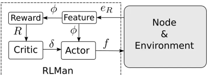
Critic Actor Reward _Node & Environment Feature RLMan

Fig. 1: Global architecture of RLMan.

environment, while minimizing the amount of reward "lost" while learning, which leads to a dilemma between exploration (learning more about the environment) and exploitation (max-imizing the reward by exploiting known information).

III. DERIVATION OFRLMAN

A policy π is evaluated by estimating the value function that can be defined in two manners. The state value function, denoted by vπ, predicts the future discounted reward if the

policy π is used to walk through the MDP from a given state, and thus evaluates the "goodness" of states [11]:

vπpeRq “ E « ₈ ÿ k“1 γk´1Rt`k ˇ ˇ ˇ ˇ St“ eR, π ff . (8)

Similarly, the action-state value function, denoted by Qπ,

evaluates the "goodness" of state-action couples when π is used [11]: QπpeR, f q “ E « ₈ ÿ k“1 γk´1R_t`k ˇ ˇ ˇ ˇ St“ eR, At“ f, π ff . (9) The EM scheme proposed in this work is an actor-critic algorithm, a class of RL techniques well-known for being ca-pable to search for optimal policies using low variance gradient estimates [12]. This class of algorithms requires storing both a representation of the value function and the policy in memory, as opposite to other techniques such as critic-only or actor-only methods, which require actor-only storing the value function or the policy respectively. Critic-only schemes require at each step deriving the policy from the value function, e.g. using a greedy method. However, this involves solving an optimization problem at each step, which may be computationally intensive, especially in the case of continuous action space and when the algorithm needs to be implemented on limited resource hardware, such as WSN nodes. On the other hand, actor-only methods work with a parametrized family of policies over which optimization procedure can be directly used, and a range of continuous action can be generated. However, these methods suffer from high variance, and therefore slow learning [12]. Actor-critic methods combine actor-only and critic-only meth-ods by storing both a parametrized representation of the policy and a value function.

Fig. 1 shows the relation between the actor and the critic. The actor updates a parametrized policy πψ, where ψ is the

policy parameter, by gradient ascent on the objective function J defined in (6). A fundamental result for computing the

gradient of J is given by the policy gradient theorem [13]: 5ψJ pπψq “ ż S ρπψpeRq ż A QπψpeR, f q 5ψπψpf | eRqdf deR “ E „ QπψpeR, f q 5ψlog πψpf | eRq ˇ ˇ ˇ ˇ ρπψ, πψ  . (10) This result reduces the computation of the performance objec-tive gradient to an expectation, and allows deriving algorithms by forming sample-based estimates of this expectation. In this work, a Gaussian policy is used to generate f :

πψpf | eRq “ 1 σ?2πexp ˜ ´pf ´ µq 2 2σ2 ¸ , (11)

where σ is fixed and controls the amount of exploration, and µ is linear with the feature:

µ “ ψφ. (12)

Defining µ as a linear function of the feature enables minimal memory footprint as only one floating value, ψ, needs to be stored. Moreover, the computational overhead is also minimal as 5ψµ “ φ, leading to:

5ψlog πψpf | eRq “

pf ´ µq

σ2 φ. (13)

It is important to notice that other ways of computing µ from the feature can be used, e.g. artificial neural networks, in which case ψ is a vector of parameters, e.g. the weight of the neural network. However, these approaches incur higher memory usage and computational overhead, and might thus not be suited for WSN nodes.

Using the policy gradient theorem as formulated in (10) may lead to high variance and slow convergence [12]. A popular way to reduce the variance is to rewrite the policy gradient theorem using the advantage function AπψpeR, f q “

Qπψ´ vπψ. Indeed, it can be shown that [13]:

5ψJ pπψq “ E „ AπψpeR, f q 5ψlog πψpf | eRq ˇ ˇ ˇ ˇ ρπψ, πψ  (14) This can reduce the variance, without changing the expectation. Moreover, the Temporal Difference (TD) error defined by:

δ “ R ` γvπψpeRq ´ vπψpe 1

Rq, (15)

is an unbiased estimate of the advantage function, and therefore can be used to compute the policy gradient [12]:

5ψJ pπψq “ E „ δ 5ψlog πψpf | eRq ˇ ˇ ˇ ˇ ρπψ, πψ  . (16)

The TD error can be intuitively interpreted as a critic of the previously taken action. Indeed, a positive TD error suggests that this action should be selected more often, while a negative TD error suggests the opposite. The critic computes the TD error (15), and, to do so, requires the knowledge of the value function vπψ. As the state space is continuous, storing the value

function for each state is not possible, and therefore function approximation is used to estimate the value function. Similarly

Algorithm 1 Reinforcement learning based energy manager. Input: eR,t, Rt 1: φt“ eR,t´ERmin Emax R ´EminR Ź Feature (3) 2: δt“ Rt` γθt´1φt´ θt´1φt´1 Ź TD Error (15), (17)

3: Ź Critic: update the value function estimate (18), (19):

4: et“ γλet´1` φt

5: θt“ θt´1` αδtet

6: Ź Actor: updating the policy (12), (13), (16):

7: ψt“ ψt´1` βδtpft´1´ψt´1φt´1q_σ2 φt´1

8: Clamp µtto rFmin, Fmaxs

9: Ź Generating a new action:

10: ft„ N pψtφt, σq

11: Clamp ft to rFmin, Fmaxs

12: return ft

to what was done for µ (12), linear function approximation was chosen to estimate the value function, as it requires very few computational overhead and memory:

ˆ

vθpeRq “ θφ, (17)

where φ is the feature (3), and θ is the approximator parameter. The critic, which estimates the value function by updating the parameter θ, is implemented using the well-known TD(λ) algorithm [14]:

et“ γλet´1` φt (18)

θt“ θt´1` αδtet (19)

where α P r0, 1s is a step-size parameter, et is a trace scalar

used to assign credit to states visited several steps earlier, and the factor λ P r0, 1q refers to the decay rate of the trace. The reader can refer to [14] for more details about this algorithm. Algorithm 1 shows the proposed EM scheme. It can be seen that the algorithm has low memory footprint and incurs low computational overhead, and therefore is suitable for execution on WSN nodes. At each run, the algorithm is fed with the current residual energy eR,t and the reward Rt computed

using (2). First, the feature and the TD error are computed (lines 1 and 2), and then the critic is updated using the TD(λ) algorithm (lines 4 and 5). Next, the actor is updated using the policy gradient theorem at line 7, where β P r0, 1s is a step-size parameter. The expectancy of the Gaussian policy is clamped to the range of allowed values at line 8. Finally, a frequency is generated using the Gaussian policy at line 10, which will be used in the current time slot. As the Gaussian distribution is unbounded, it is required to clamp the generated value to the allowed range (line 11).

IV. EVALUATION OFRLMAN

RLMan was evaluated and compared to three state-of-the-art EMs using exhaustive simulations. The simulated platform was PowWow [15], a modular WSN platform designed for en-ergy harvesting. The PowWow platform uses a supercapacitor as energy storage device, with a maximum voltage of 5.2V and a failure voltage of 2.8 V. The harvested energy was simulated by two energy traces from real measurements: one lasting 270

All Etyp_C 8.672 mJ Emax C 36.0 mJ Fmin 1 300Hz Fmax _{5 Hz} T 60 s RLMan α 0.1 β 0.01 σ 0.1 γ 0.9 λ 0.9 P-FREEN [8] BOF L 0.95E max R η 1.0 Fuzzyman [10] K 1.0 η 1.0 Eeds_B FminT Etyp_c Emin_B FminT Etyp_c Estrong_H FmaxT E_ctyp E_Hweak FminT Etyp_c

LQ-Tracker [4]

µ 0.001 B˚ 0.70Emax_R

α 0.5 β 1.0

TABLE I: Parameter values used for simulations. For details about the parameters of P-FREEN, Fuzzyman and LQ-Tracker, the reader can refer to the respective literature.

days corresponding to indoor light [16] and the other lasting 180 days corresponding to outdoor wind [17], allowing the evaluation of the EM schemes for two different energy source types. The task of the node consists of acquiring data by sensing, performing computation and then sending the data to a sink. However, in practice, the amount of energy consumed by one execution of this task varies, e.g. due to multiple retransmissions. Therefore, the amount of energy required to run one execution was simulated by a random variable which follows a beta distribution, with the mode of the distribution set to the energy consumed if only one transmission attempt is required, denoted by E_Ctyp, and the maximum set to the energy consumed if five transmission attempts are necessary, denoted by Emax_C . Table I shows the values of E_Ctypand E_Cmax, as well as the parameter values used when implementing the EMs. The rest of this section is organized as follows. First, preliminary results detail the behavior of the learning phase of the proposed algorithm, focusing on the first few days. Next, the comparison results of the proposed EM with three state-of-the-art schemes are exposed.

A. Preliminary results

Fig. 2 shows the behavior of the proposed EM during the first 30 days of simulation using the indoor light energy trace. The capacitance of the energy storage device was set to 0.5 F. Fig. 2a shows the harvested power, and Fig. 2b shows the feature (φ), corresponding to the normalized residual energy. Fig. 2c exposes the expectancy of the Gaussian distribution used to generate the throughput (µ), and Fig. 2d shows the reward (R), computed using (2). It can be seen that the first

0 5 10 15 20 25 30 Time (days) 0.0 0.2 0.4 0.6 0.8 1.0 Harvested Power (mW)

(a) Harvested power from indoor light.

0 5 10 15 20 25 30 Time (days) 0.2 0.3 0.4 0.5 0.6 0.7 0.8 0.9 1.0 Fe at ur e φ

(b) Feature (state of charge of the energy storage device).

0 5 10 15 20 25 30 Time (days) 0.00 0.01 0.02 0.03 0.04 0.05 Po lic y e xp ec ta nc y µ (H z)

(c) Gaussian policy expectation.

0 5 10 15 20 25 30 Time (days) 0 10 20 30 40 50 Re wa rd R (d) Reward. Fig. 2: Behavior of the EM scheme the first 30 days.

day the energy storage device was saturated (Fig. 2b), as the average throughput was progressively increasing (Fig. 2c), leading to higher rewards (Fig. 2d). As during the second and third days the amount of harvested energy was low, the residual energy dropped, causing a decrease of the rewards while the policy expectancy was stable. Starting the fourth day, energy was harvested again, enabling the node to increase its activity, as it can be seen on Fig. 2c. Finally, it can be noticed that if a lot of energy was wasted by saturation of the energy storage device the first 5 days, this is no longer true once this period of learning is over.

B. Comparison to state-of-the-art

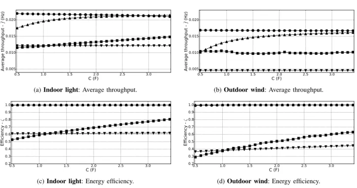
RLMan was compared to P-FREEN, Fuzzyman, and LQ-Tracker, three state-of-the-art EM schemes that aim to maximize the throughput. P-FREEN and Fuzzyman require the tracking of the harvested energy in addition to the residual energy, and were therefore executed with perfect knowledge of this value. RLMan and LQ-Tracker were only fed with the value of the residual energy. Both the indoor light and the wind energy traces were considered. The EMs were evaluated for different values of capacitances, ranging from 0.5F to 3.5F, as it strongly impacts the behavior of the EMs, but also both the cost and form factor of WSN nodes. In addition to the average throughput, the energy efficiency denoted by ζ was also evaluated, and is defined by:

ζ “ 1 ´ ř teW,t ř teH,t , (20)

where eW,t is the energy wasted by saturation of the energy

storage device during the tth time slot, i.e. the energy that could not be stored because the energy storage device was full, and eH,t is the energy harvested during the tth time

slot. Moreover, each data point is the average of the results

of ten simulations, each performed using different seeds for the random number generators.

All the EMs successfully avoid power failure when pow-ered by indoor light or outdoor wind. Fig. 3 exposes the com-parison results. As it can be seen on Fig 3c and Fig. 3d, both RLMan and LQ-Tracker achieve more than 99.9 % efficiency, for indoor light and outdoor wind, for all capacitance values, and despite the fact that they require only the residual energy as an input. In addition, when the node is powered by outdoor wind, RLMan always outperforms the other EMs in terms of average throughput for all capacitance values, as shown by Fig. 3b. When the node is powered by indoor light, RLMan also outperforms all the other EMs, except LQ-Tracker when the values of the capacitance are higher than 2.8 F. Moreover, the advantage of RLMan over the other EMs is more significant for small values of the capacitance. Especially, the average throughput is more than 20 % higher compared to LQ-Tracker in the case of indoor light, and almost 70 % higher in the case of outdoor wind, when the capacitance value is set to 0.5 F. This is encouraging as using small capacitance leads to lower cost and lower form factor.

V. CONCLUSION

In this paper, the problem of maximizing the quality of service in energy harvesting node is formulated using rein-forcement learning theory, and a novel energy management scheme, named RLMan, is presented. RLMan requires only the state of charge of the energy storage device as an input, and uses function approximation to minimize the memory footprint and the computational overhead, which makes it practical to implement and suitable for wireless sensor nodes. Exhaustive simulations showed the benefits enabled by RLMan in terms of throughput and energy efficiency compared to three state-of-the-art energy managers, in the case of both indoor

0.5 1.0 1.5 2.0 2.5 3.0 C (F) 0.005 0.010 0.015 0.020 Av er ag e t hr ou gh pu t -¯ f (H z)

(a) Indoor light: Average throughput.

0.5 1.0 1.5 2.0 2.5 3.0 C (F) 0.005 0.010 0.015 0.020 Av er ag e t hr ou gh pu t -¯ f (H z)

(b) Outdoor wind: Average throughput.

0.5 1.0 1.5 2.0 2.5 3.0 C (F) 0.2 0.3 0.4 0.5 0.6 0.7 0.8 0.9 1.0 Ef fic ien cy - ζ

(c) Indoor light: Energy efficiency.

0.5 1.0 1.5 2.0 2.5 3.0 C (F) 0.2 0.3 0.4 0.5 0.6 0.7 0.8 0.9 1.0 Ef fic ien cy - ζ

(d) Outdoor wind: Energy efficiency.

Fig. 3: Average throughput and energy efficiency for different capacitance values, in the case of indoor light and outdoor wind.

light energy harvesting and outdoor wind energy harvesting. The advantage of RLMan is more significant when small energy storage devices are used. We have identified areas of potential improvement, including the exploration of other rewards and other function approximators, which may lead to faster convergence.

REFERENCES

[1] R. Margolies, M. Gorlatova, J. Sarik, G. Stanje, J. Zhu, P. Miller, M. Szczodrak, B. Vigraham, L. Carloni, P. Kinget, I. Kymissis, and G. Zussman, “Energy-Harvesting Active Networked Tags (EnHANTs): Prototyping and Experimentation,” ACM Transactions on Sensor Net-works, vol. 11, no. 4, pp. 62:1–62:27, November 2015.

[2] M. Magno, L. Spadaro, J. Singh, and L. Benini, “Kinetic Energy Harvesting: Toward Autonomous Wearable Sensing for Internet of Things,” in International Symposium on Power Electronics, Electrical Drives, Automation and Motion (SPEEDAM), June 2016, pp. 248–254. [3] A. Kansal, J. Hsu, S. Zahedi, and M. B. Srivastava, “Power Manage-ment in Energy Harvesting Sensor Networks,” ACM Transactions on Embedded Computing Systems, vol. 6, no. 4, 2007.

[4] C. M. Vigorito, D. Ganesan, and A. G. Barto, “Adaptive Control of Duty Cycling in Energy-Harvesting Wireless Sensor Networks,” in 4th Annual IEEE Communications Society Conference on Sensor, Mesh and Ad Hoc Communications and Networks (SECON), June 2007. [5] A. Castagnetti, A. Pegatoquet, C. Belleudy, and M. Auguin, “A

Frame-work for Modeling and Simulating Energy Harvesting WSN Nodes with Efficient Power Management Policies,” EURASIP Journal on Embedded Systems, no. 1, 2012.

[6] T. N. Le, A. Pegatoquet, O. Berder, and O. Sentieys, “Energy-Efficient Power Manager and MAC Protocol for Multi-Hop Wireless Sensor Networks Powered by Periodic Energy Harvesting Sources,” IEEE Sensors Journal, vol. 15, no. 12, pp. 7208–7220, 2015.

[7] R. C. Hsu, C. T. Liu, and H. L. Wang, “A Reinforcement Learning-Based ToD Provisioning Dynamic Power Management for Sustainable Operation of Energy Harvesting Wireless Sensor Node,” IEEE

Trans-actions on Emerging Topics in Computing, vol. 2, no. 2, pp. 181–191, June 2014.

[8] S. Peng and C. P. Low, “Prediction free energy neutral power manage-ment for energy harvesting wireless sensor nodes,” Ad Hoc Networks, vol. 13, Part B, 2014.

[9] F. Ait Aoudia, M. Gautier, and O. Berder, “GRAPMAN: Gradual Power Manager for Consistent Throughput of Energy Harvesting Wireless Sensor Nodes,” in IEEE 26th Annual International Symposium on Personal, Indoor, and Mobile Radio Communications (PIMRC), August 2015.

[10] ——, “Fuzzy Power Management for Energy Harvesting Wireless Sensor Nodes,” in IEEE International Conference on Communications (ICC), May 2016.

[11] H. Van Hasselt, “Reinforcement Learning in Continuous State and Action Spaces,” in Reinforcement Learning. Springer, 2012, pp. 207– 251.

[12] I. Grondman, L. Busoniu, G. A. D. Lopes, and R. Babuska, “A Survey of Actor-Critic Reinforcement Learning: Standard and Natural Policy Gradients,” IEEE Transactions on Systems, Man, and Cybernetics, Part C (Applications and Reviews), vol. 42, no. 6, pp. 1291–1307, November 2012.

[13] R. S. Sutton, D. A. McAllester, S. P. Singh, and Y. Mansour, “Policy Gradient Methods for Reinforcement Learning with Function Approx-imation.” in Advances in Neural Information Processing Systems 12, vol. 99, 2000, pp. 1057–1063.

[14] R. S. Sutton, “Learning to Predict by the Methods of Temporal Differences,” Machine Learning, vol. 3, no. 1, pp. 9–44, 1988. [15] O. Berder and O. Sentieys, “PowWow : Power Optimized

Hard-ware/Software Framework for Wireless Motes,” in International Con-ference on Architecture of Computing Systems (ARCS), February 2010, pp. 1–5.

[16] M. Gorlatova, A. Wallwater, and G. Zussman, “Networking Low-Power Energy Harvesting Devices: Measurements and Algorithms,” in IEEE INFOCOM, April 2011.

[17] “NREL: MIDC - National Wind Technology Center,” http://www.nrel.gov/midc/nwtc_m2/.