HAL Id: hal-00297103
https://hal.archives-ouvertes.fr/hal-00297103
Submitted on 10 Apr 2008
HAL is a multi-disciplinary open access
archive for the deposit and dissemination of
sci-entific research documents, whether they are
pub-lished or not. The documents may come from
teaching and research institutions in France or
abroad, or from public or private research centers.
L’archive ouverte pluridisciplinaire HAL, est
destinée au dépôt et à la diffusion de documents
scientifiques de niveau recherche, publiés ou non,
émanant des établissements d’enseignement et de
recherche français ou étrangers, des laboratoires
publics ou privés.
El Niño ? related precipitation variability in Perú
P. Lagos, Y. Silva, E. Nickl, K. Mosquera
To cite this version:
P. Lagos, Y. Silva, E. Nickl, K. Mosquera. El Niño ? related precipitation variability in Perú. Advances
in Geosciences, European Geosciences Union, 2008, 14, pp.231-237. �hal-00297103�
www.adv-geosci.net/14/231/2008/ © Author(s) 2008. This work is licensed under a Creative Commons License.
Geosciences
El Ni ˜no – related precipitation variability in Per ´u
P. Lagos1, Y. Silva1, E. Nickl2, and K. Mosquera11Instituto Geof´ısico del Per´u, Lima, Per´u
2Department of Geography, University of Delaware, Delaware, USA
Received: 15 July 2007 – Revised: 19 November 2007 – Accepted: 19 November 2007 – Published: 10 April 2008
Abstract. The relationship between monthly mean sea
sur-face temperature (SST) anomalies in the commonly used El Ni˜no regions and precipitation for 44 stations in Per´u is doc-umented for 1950–2002. Linear lag correlation analysis is employed to establish the potential for statistical precipita-tion forecasts from SSTs. Useful monthly mean precipitaprecipita-tion anomaly forecasts are possible for several locations and cal-endar months if SST anomalies in El Ni˜no 1+2, Ni˜no 3.4, and Ni˜no 4 regions are available. Prediction of SST anomalies in El Ni˜no regions is routinely available from Climate Predic-tion Center, NOAA, with reasonable skill in the El Ni˜no 3.4 region, but the prediction in El Ni˜no 1+2 region is less reli-able. The feasibility of using predicted SST anomalies in the El Ni˜no 3.4 region to predict SST anomalies in El Ni˜no 1+2 region is discussed.
1 Introduction
El Ni˜no in Peru is characterized by above normal sea surface temperatures (SSTs) along the coast and heavy precipitation in the northern coastal desert.
The warming and rains typically begin just after Christ-mas, hence the name El Ni˜no or “the boy.” Originally the term El Ni˜no was used by sailors in the Paita area (5◦S) to
describe a narrow current of warm surface water that moves south from Ecuador beginning at this time in most years and lasting several months (Carrillo, 1892). Studies of the ocean and weather conditions during the 1960s emphasized the anomalous warm years, and referred to those episodes as El Ni˜nos. Bjerknes (1966, 1969) documented coherent warm equatorial SST anomalies from the dateline to the Ecuador coast, and related this feature to both the warming at the
Correspondence to: P. Lagos
Peru coast and to planetary-scale changes in the tropical at-mosphere, the “Southern Oscillation”.
In subsequent years, the term “El Ni˜no” has been used in the literature to describe basin-scale equatorial Pacific warm-ings, and this has blurred the distinction with the coastal phenomenon, which while related to does not exhibit a one-to-one correspondence with the basin-scale SST variability (Rasmusson and Carpenter, 1982; Deser and Wallace, 1987; Trenberth and Stepaniak, 2001). This usage has lead to con-fusion and contradictions in the use of the term “El Ni˜no” (Aceituno, 1992). In 1983 a Scientific Committee for Ocean Research (SCOR) working group 55 defined El Ni˜no as “El Ni˜no is the appearance of anomalously warm water along the coast of Ecuador and Per´u as far south as Lima (12◦S). This
means a normalized sea surface temperature (SST) anomaly exceeding one standard deviation for at least four (4) consec-utive months. This normalized SST anomaly should occur at least at three (3) of five (5) Peruvian coastal stations”, a definition that was equivalent to that used by Peruvian re-searchers, but it was not accepted by the international sci-entific community. Trenberth (1977) has explored possible definitions of El Ni˜no and concluded that the definition is still evolving and alternative criteria might be used.
SST anomalies in the region 5◦N to 5◦S, 170–120◦W
(Fig. 1), referred to as “Ni˜no 3.4”, relate well to changes in the Northern Hemisphere extratropical winter circulation, and are also predictable to a useful degree by mechanistic and statistical models. For these reasons, NOAA’s NWS Cli-mate Services Division has adopted an operational definition for El Ni˜no for monitoring and prediction purposes which is based on Ni˜no 3.4 SST anomalies (3-month average SST anomaly >=0.5C with respect to 1971–2000). The definition is at http://www.noaanews.noaa.gov/stories2005/s2394.htm. When the area of interest is the South American Pacific coast, the NOAA definition differs from the local concept of El Ni˜no which is equivalent to the SCOR definition. Also when the SST anomaly in the El Ni˜no 3.4 region meets the
232 P. Lagos et al.: El Ni˜no – related precipitation variability in Per´u
Fig. 1. Location of El Ni˜no regions.
NOAA’s El Ni˜no criterion, the SST anomaly in the El Ni˜no 1+2 region may be smaller in amplitude, and hence an an-nouncement of an El Ni˜no event based on the NOAA defini-tion leads to confusion among the Peruvian public, such as in the year 2003 and 2006. In this study, SST variations in El Ni˜no 3.4 and El Ni˜no 1+2 regions will be distinguished. In addition, numerous studies have examined the efficacy of El Ni˜no/Southern Oscillation (ENSO)-related SST anomalies in various parts of the central and western equatorial Pacific to forcing atmospheric teleconnections (for example, Bar-sugli and Sardeshmukh 2002), but fewer studies have doc-umented the relative importance of coastal- and basin-wide SST anomalies in forcing precipitation over Peru (Deser and Wallace, 1987; Nickl, 2007). Finally the present study doc-uments the ENSO and El Ni˜no signatures in Peru in greater geographic detail than in previous studies.
In Per´u, precipitation occurs along the northern coast dur-ing El Ni˜nos, in the Andes and the Amazon in all years, and significant precipitation does not occur along the central and southern coast. The beginning and end of the precipi-tation seasons varies slightly from one region, and will be discussed in Sect. 4. The onset and intensity of precipitation varies from year to year, and in some years the variability can take the form of an extreme event, such as heavy or deficit of precipitation, which evolves into a natural disaster. Extreme precipitation events in the Andes have been associated by lo-cal investigators and, particularly by the lolo-cal media, with El Ni˜no events, despite the fact that the linkage between these climate events and El Ni˜no has not been established.
Many studies have documented the variability of precipi-tations in different zones of South America and their relation with the basin-scale El Ni˜no (Aceituno, 1988, 1989; Diaz et al., 1998; Grimm et al., 2000, 2002; Montecinos et al., 2000; Pisciottano et al., 1994). One of the most studied regions is the Amazon (Liebmann and Marengo, 2001; Marengo et al., 2001), but few have been made for the Andes (Vuille, et al., 2000; Villacis, 2001). The work of Ropelewski and Halpert (1987, 1989) related precipitation over broad regions of South America to ENSO.
In this paper the relationship between Per´u precipitation and Per´u-coast and basin-wide SST anomalies for 1950– 2002 is characterized with linear lag correlation coefficients. The goal is to establish the potential for statistical
precip-itation forecasts based on SST anomalies in the Ni˜no 1+2 and 3.4 regions. The following sections describe the data, methodology, annual cycle and interannual variability, and the development of the forecast model.
2 Data
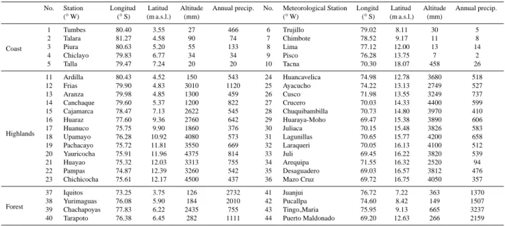
Monthly precipitations totals for 44 stations and the years 1950 to 2002 were selected for the study. Twenty-three of the stations are located at airports and belong to the Peru-vian Corporation of Civil Aviation (CORPAC), and the data for the other 21 stations were compiled by the IGP from dif-ferent sources. Precipitation anomalies are calculated with respect to 1961–1990. Table 1 lists the stations employed in the study.
Monthly values of the El Ni˜no 1+2, Ni˜no 3, Ni˜no 3.4, and Ni˜no 4 SST indices were obtained from the NOAA Cli-mate Prediction Center WWW site and are derived from the NOAA optimal interpolation SST dataset (Reynolds and Smith, 1994). Anomalies are with respect to a 1961-90 cli-matology.
3 Methodology
Pearson linear lag correlation analysis is employed to relate precipitation to SST indices for the El Ni˜no 1+2, Ni˜no 3, Ni˜no 3,4 and Ni˜no 4 regions. Two-dimensional correlation and scatter plots are also constructed to illustrate the rela-tionship between El Ni˜no 1+2 and Ni˜no 3.4 indices.
4 Annual cycle
A knowledge of the annual cycle of precipitation over the Pe-ruvian region is necessary for understanding the interannual variability, which is the focus of this study. Precipitation in the Andes begins in September and ends in May, with maxi-mum values in the months of January–March, rapid diminu-tion in April, and slight variadiminu-tions from stadiminu-tion to stadiminu-tion. In the extreme northern coast, seasonal precipitation begins during El Ni˜nos around November and ends around March. In the remainder of the coastal regions precipitation does not occur, and in the Amazon basin precipitation begins around August and ends around June.
The annual cycle of precipitation in the Peruvian Andes is associated with the seasonal displacement of the South Pa-cific and South Atlantic anticyclones, the north-south sea-sonal displacement of the Intertropical Convergence Zone, humidity transport from the Amazon, and with the formation of a center of high pressure in high levels of the atmosphere, known as the Bolivian High (Virji, 1981; Silva Dias et al., 1983). The spatial and temporal variability of seasonal pre-cipitation in the Andean region is similar to that observed in the rest of South America (Figueroa and Nobre, 1990).
Table 1. List of meteorological station.
No. Station Longitud Latitud Altitude Annual precip. No. Meteorological Station Longitd Latitud Altitude Annual precip.
(◦W) (◦S) (m a.s.l.) (mm) (◦W) (◦S) (m a.s.l.) (mm) Coast 1 Tumbes 80.40 3.55 27 466 6 Trujillo 79.02 8.11 30 5 2 Talara 81.27 4.58 90 74 7 Chimbote 78.52 9.17 11 8 3 Piura 80.63 5.20 55 133 8 Lima 77.12 12.00 13 14 4 Chiclayo 79.83 6.77 34 34 9 Pisco 76.28 13.75 7 2 5 Talla 79.47 7.24 20 20 10 Tacna 70.30 18.07 458 26 Highlands 11 Ardilla 80.43 4.52 150 543 24 Huancavelica 74.98 12.78 3680 518 12 Frias 79.90 4.83 3010 1120 25 Ayacucho 74.22 13.13 2749 527 13 Aranza 79.98 4.85 1300 459 26 Cusco 71.98 13.55 3249 737 14 Canchaque 79.60 5.37 1200 822 27 Crucero 70.03 14.33 4400 599 15 Cajamarca 78.47 7.13 2622 545 28 Chuquibambilla 70.73 14.80 3970 410 16 Huaraz 77.60 9.36 2760 642 29 Huaraya-Moho 69.47 15.38 3890 606 17 Huanuco 75.75 9.90 1860 376 30 Juliaca 70.15 15.48 3826 583 18 Upamayo 76.28 10.92 4080 573 31 Lagunillas 70.65 15.77 4200 658 19 Pachacayo 75.72 11.81 3550 669 32 Laraqueri 70.05 16.13 4100 512 20 Yauricocha 75.91 11.96 4375 814 33 Juli 69.45 16.22 3820 539 21 Huayao 75.32 12.03 3313 755 34 Arequipa 71.55 16.32 2520 94 22 Pampas 74.87 12.39 3260 542 35 Desaguadero 69.03 16.57 3812 476
23 Chichicocha 75.61 12.17 4500 437 36 Mazo Cruz 69.72 16.75 4050 357
Forest
37 Iquitos 73.25 3.75 126 2732 41 Juanjui 76.72 7.22 363 1370
38 Yurimaguas 76.08 5.90 184 2010 42 Pucallpa 74.60 8.42 149 1507
39 Chachapoyas 77.83 6.22 2435 755 43 Tingo Maria 75.95 9.13 665 3237
40 Tarapoto 76.38 6.45 282 1111 44 Puerto Maldonado 69.20 12.63 266 2159
5 Interanual variability
The precipitation indices exhibit large variability from month to month and year to year. For visualization purposes, a smooth time series is obtained by applying a six-month run-ning mean to the time series. Figure 2 shows the results for six representative Andean stations. The time series are domi-nated by interannual variability, where very humid years and very dry years are taken as those where the precipitation in-dices exceed plus and minus one standard deviation (horizon-tal lines). The causes of the interannual variability of precip-itation will be discussed elsewhere.
6 Correlation analysis
6.1 Equatorial Pacific SST and precipitation
Correlation analysis between each of the 44 precipitation indices and the 4 SST anomaly indices, corresponding to the regions Ni˜no 1+2, Ni˜no 3, Ni˜no 3.4, and Ni˜no 4, has been performed for each calendar month in the climatolog-ical rainy season of October to March. The output of the analysis is presented both in Table 2 and Figs. 3–5.
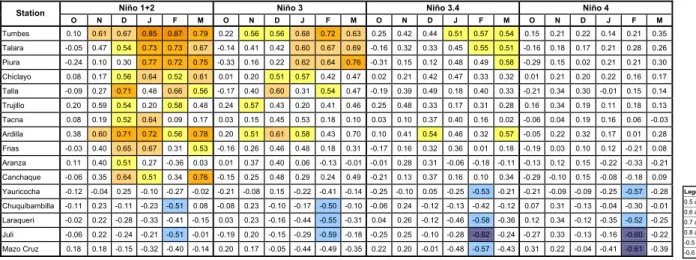
Table 2 is simplified by only listing values for stations where the correlation magnitude is >=0.5. Shading is em-ployed in the table to draw attention to the strongest rela-tionships. From this table one can identify three Andean subregions with different climatic characteristics. The cor-relation coefficients between the precipitation indices in the Andean region and the SST anomaly indices for El Ni˜no re-gion 1+2 are moderately positive (the precipitation tends to
Fig. 2. Six months running mean series for six representative pre-cipitations indices (mm/month).
234 P. Lagos et al.: El Ni˜no – related precipitation variability in Per´u
Table 2. Linear correlation coefficients between SST anomaly indices for El Ni˜no regions and precipitation.
Niño 1+2 Niño 3 Niño 3.4 Niño 4
Station O N D J F M O N D J F M O N D J F M O N D J F M Tumbes 0.10 0.61 0.67 0.85 0.87 0.79 0.22 0.56 0.56 0.68 0.72 0.63 0.25 0.42 0.44 0.51 0.57 0.54 0.15 0.21 0.22 0.14 0.21 0.35 Talara -0.05 0.47 0.54 0.73 0.73 0.67 -0.14 0.41 0.42 0.60 0.67 0.69 -0.16 0.32 0.33 0.45 0.55 0.51 -0.16 0.18 0.17 0.21 0.28 0.26 Piura -0.24 0.10 0.30 0.77 0.72 0.75 -0.33 0.16 0.22 0.62 0.64 0.76 -0.31 0.15 0.12 0.48 0.49 0.58 -0.29 0.15 0.02 0.21 0.21 0.30 Chiclayo 0.08 0.17 0.56 0.64 0.52 0.61 0.01 0.20 0.51 0.57 0.42 0.47 0.02 0.21 0.42 0.47 0.33 0.32 0.01 0.21 0.20 0.22 0.16 0.17 Talla -0.09 0.27 0.71 0.48 0.66 0.56 -0.17 0.40 0.60 0.31 0.54 0.47 -0.19 0.39 0.49 0.18 0.40 0.33 -0.21 0.34 0.30 -0.01 0.15 0.14 Trujillo 0.20 0.59 0.54 0.20 0.58 0.48 0.24 0.57 0.43 0.20 0.41 0.46 0.25 0.48 0.33 0.17 0.31 0.28 0.16 0.34 0.19 0.11 0.18 0.13 Tacna 0.08 0.19 0.52 0.64 0.09 0.17 0.03 0.15 0.45 0.53 0.18 0.10 0.03 0.10 0.37 0.40 0.16 0.02 -0.06 0.04 0.19 0.16 0.06 -0.03 Ardilla 0.38 0.60 0.71 0.72 0.56 0.78 0.20 0.51 0.61 0.58 0.43 0.70 0.10 0.41 0.54 0.46 0.32 0.57 -0.05 0.22 0.32 0.17 0.01 0.28 Frias -0.03 0.40 0.65 0.67 0.31 0.53 -0.16 0.26 0.46 0.48 0.18 0.31 -0.17 0.16 0.32 0.36 0.01 0.18 -0.19 0.03 0.10 0.12 -0.21 0.08 Aranza 0.11 0.40 0.51 0.27 -0.36 0.03 0.01 0.37 0.40 0.06 -0.13 -0.01 -0.01 0.28 0.31 -0.06 -0.18 -0.11 -0.13 0.12 0.15 -0.22 -0.33 -0.21 Canchaque -0.06 0.35 0.64 0.51 0.34 0.76 -0.15 0.25 0.48 0.29 0.24 0.49 -0.21 0.13 0.37 0.16 0.10 0.34 -0.29 -0.10 0.15 -0.08 -0.18 0.09 Yauricocha -0.12 -0.04 0.25 -0.10 -0.27 -0.02 -0.21 -0.08 0.15 -0.22 -0.41 -0.14 -0.25 -0.10 0.05 -0.25 -0.53 -0.21 -0.21 -0.09 -0.09 -0.25 -0.57 -0.28 Chuquibambilla -0.11 0.23 -0.11 -0.23 -0.51 0.08 -0.08 0.23 -0.10 -0.17 -0.50 -0.10 -0.06 0.24 -0.12 -0.13 -0.42 -0.12 0.07 0.31 -0.13 -0.04 -0.30 -0.01 Laraqueri -0.02 0.22 -0.28 -0.33 -0.41 -0.15 0.03 0.23 -0.16 -0.44 -0.55 -0.31 0.04 0.26 -0.12 -0.46 -0.58 -0.36 0.12 0.34 -0.12 -0.35 -0.52 -0.25 Juli -0.06 0.22 -0.24 -0.21 -0.51 -0.01 -0.19 0.20 -0.15 -0.29 -0.59 -0.18 -0.25 0.25 -0.10 -0.28 -0.62 -0.24 -0.27 0.33 -0.13 -0.16 -0.60 -0.22 Mazo Cruz 0.18 0.18 -0.15 -0.32 -0.40 -0.14 0.20 0.17 -0.05 -0.44 -0.49 -0.35 0.22 0.20 -0.01 -0.48 -0.57 -0.43 0.31 0.22 -0.04 -0.41 -0.61 -0.39 Legend: 0.5 a 0.6 0.6 a 0.7 0.7 a 0.8 0.8 a 0.9 -0.5 a -0.6 -0.6 a -0.7
gions and precipitation
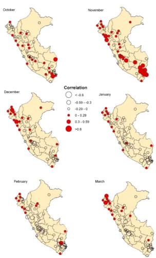
Fig. 3. Correlation between precipitation indices and SST anomaly
indices in El Ni˜no 1+2 region. Fig. 4. Correlation between precipitation indices and SST anomaly indices in El Ni˜no 3.4 region.
be greater than the average during El Ni˜no) in the north end of the northern subregion during November–March. The cor-relation coefficients are neutral in the central subregion, but moderately positive in November, and are slightly negative (the precipitation tends to be smaller than average during El Ni˜nos) in the southern subregion, but moderately negative in February.
The correlation coefficients between the precipitation in-dices in the Andes and the SST anomaly inin-dices for El Ni˜no region 3.4 are weakly positive in the northern subregion, neu-tral in the cenneu-tral subregion and moderately negative in the southern subregion, particularly in February. The correlation coefficients between the precipitation indices and the SST anomaly indices for El Ni˜no 4 region are very small in the north and moderately negative in the central and south sub-regions, particularly in February.
The correlation analysis indicates that precipitation in the northern coast is strongly related to the SST anomaly indices for El Ni˜no region 1+2, mainly in the period January–March. During El Ni˜no events, as defined by SCOR, the relationship intensifies, confirming the results of previous studies (Wood-man, 1999, and numerous others). The correlation coeffi-cients between the precipitation indices in the Peruvian Ama-zon region and the SST anomaly indices for the four El Ni˜no regions are small in magnitude.
Figure 3 depicts the correlation between the precipitation indices and SST anomalies for the El Ni˜no 1+2 region for the calendar months October to March. Figures 4 and 5 show the results of the correlation between precipitation indices and SST anomaly indices for El Ni˜no 3.4 and El Ni˜no 4 regions, respectively. In these figures the magnitudes of the corre-lation coefficients are indicated by the size of the open and shaded circles. Stronger positive correlations, represented as large shaded circles, are shown in Fig, 3 for the northern coast from November to March. Similarly, in Fig. 4 moderate positive correlations are observed in the northern coast from November to March, and in Fig. 5 moderate positive corre-lations are observed along the Andean region in November. Moderate negative correlations with both El Ni˜no 3.4 and El Ni˜no 4 are observed along the Andean region in January, February and March (Figs. 4 and 5).
6.2 Precipitation forecast in Peru
The forecast of monthly precipitation anomalies in Per´u re-lies on the correlation analysis presented in this paper and on the prediction of SST anomalies in El Ni˜no regions. Most of the international effort in predicting SST anomalies in the equatorial Pacific has been focused in El Ni˜no 3.4 region since large positive and negative SST anomalies in this re-gion has global climatic consequences and relatively little at-tention has been given to the prediction of SST anomalies, for example, in the El Ni˜no 1+2 region. This is probably due to the fact that the ability to predict SST anomalies in El Ni˜no 3.4 region is higher than in El Ni˜no 1+2 region, due to
Fig. 5. Correlation between precipitation indices and SST anomaly indices in El Ni˜no 4 region.
a more complex physics processes involved in El Ni˜no 1+2 region than in El Ni˜no 3.4 region.
SST anomaly forecasts for El Ni˜no 3.4 regions are rou-tinely available from the NOAA Climate Prediction Center and, if we assume that SST anomalies in El Ni˜no 3.4 are rep-resentative of SST anomalies over the entire equatorial Pa-cific, precipitation anomalies can be forecast for Per´u. The correlation analysis of Sect. 6.1 documents the greater sen-sitivity of north coastal precipitation anomalies to local SST anomalies than to basin-scale SST variations, which suggests the usefulness of predicting El Ni˜no 1+2 SST variability. To investigate the extent to which one can use SST anomalies in El Ni˜no 3.4 region to predict SST anomalies in the El Ni˜no 1+2 region, a linear lag correlation analysis between SST anomaly in El Ni˜no 3.4 and El Ni˜no 1+2 regions has been performed.
Table 3 shows the lagged correlation coefficients between SST anomaly indices in El Ni˜no 3.4 and El Ni˜no 1+2 regions for six calendar months for the years 1950–2006. Each row is the correlation between Ni˜no 3.4 in a specific calendar month and Ni˜no 1+2 for months preceding, simultaneous to, or
fol-236 P. Lagos et al.: El Ni˜no – related precipitation variability in Per´u
Table 3. Lagged correlation coefficients between SSTA indices in El Ni˜no 3.4 and El Ni˜no 1+2 regions for six calendar month.
M 0.748 0.697 0.678 0.541 0.504 0.534 0.441 F 0.763 0.778 0.740 0.653 0.504 0.463 0.468 J 0.775 0.808 0.820 0.714 0.598 0.384 0.326 D 0.676 0.779 0.822 0.822 0.750 0.572 0.286 N 0.602 0.688 0.804 0.825 0.832 0.741 0.563 O 0.531 0.613 0.697 0.812 0.836 0.841 0.741 -3 -2 -1 0 1 2 3 Lag (month)
e 3. Lagged correlation coefficients between SSTA indices in El Niño 3.4 and El Niño 1+2 reg
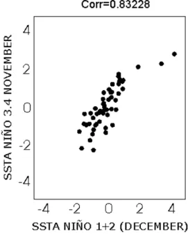
lowing that month. The month of largest correlation magni-tude in each row is shaded. Positive lags are months where Ni˜no 1+2 follows Ni˜no 3.4. The results indicate that SST anomalies in the El Ni˜no 3.4 region in October and Novem-ber could be used to predict DecemNovem-ber SST anomalies in the El Ni˜no 1+2 region. Table 3 also indicates December SST anomaly predictions for the El Ni˜no 3.4 region could be used to predict December SST anomalies in El Ni˜no 1+2 region. It is also suggestive from Table 3 that the SST anomalies prop-agates from west to east during October and November and propagates from east to west during January to March. To test the sensitivity of Table 3 to conditions before and after the 1976–1977 climate regime shift (Mantua et al., 1997), we repeated the analysis for the periods 1950–1976 and 1977– 2006, and found no substantial difference from those shown in Table 3. Figure 6 is a scatter plot between November El Ni˜no 3.4 and December El Ni˜no 1+2 SST anomalies. A lin-ear model of the relation between these two indices would underestimate the magnitude of the Ni˜no 1+2 anomaly in the extreme warm years.
Precipitation forecast in the Andean region based on the prediction of SST anomaly in El Ni˜no 3.4 regions is possi-ble for several locations where the correlation coefficient is moderately large in magnitude. Note that the negative corre-lation improves, particularly in the southern Andean region, when SST anomaly indices for El Ni˜no 4 region are used (Fig. 5), however the prediction of SST anomalies for the El Ni˜no 4 region has limitation and this topic will be discussed elsewhere.
7 Conclusions and discussion
Monthly precipitation data from 44 Peruvian stations and SST anomaly indices for the 4 El Ni˜no regions in the
equa-Fig. 6. Scatter plot and correlation coefficient of SSTA indices in El Ni˜no 1+2 (December) and El Ni˜no 3.4 (November) regions.
torial Pacific are used to perform linear correlation analysis with the purpose of establishing the potential for statistical forecasting of monthly precipitation totals in Per´u.
The results of the study reveal the following:
– Three subregions with different El Ni˜no precipitation
regimes exist in the Andean mountain region, and they are located in the north, center and south of Per´u.
– Interannual variability of precipitation is the dominant
time scale feature.
– Precipitation extremes in the northern coast of Peru are
highly and positively correlated with SST anomalies in El Ni˜no 1+2 region, warm SST forcing precipitation ex-cesses, as several investigators have found.
– Precipitation extremes in the southern Andean region
are moderately correlated with SST anomalies in the El Ni˜no 4 region, with positive correlations in November and negative correlations from January to March. The negative correlations, warm SST leading precipitation deficit, is associated with teleconnection mechanism as discussed by Nickl (2007).
– Precipitation forecast in the Andean region based on the
prediction of SST anomalies in El Ni˜no 3.4 regions is possible for several locations in Per´u where the correla-tion coefficients are moderately high.
– Considering that precipitation in the northern coast of
Per´u is only significant from December to March dur-ing warm SSTs in the El Ni˜no 1+2 region, precipitation
forecasts in the northern coast for December are pos-sible using the predicted SST anomaly in the El Ni˜no 3.4 region. For extreme warm events, when the SST anomalies in El Ni˜no 3.4 exceed 1◦C and in the months
when the correlation between both SST anomaly indices is largest, precipitation forecasts for January through March are possible using the predicted SST anomaly in El Ni˜no 3.4 region.
Acknowledgements. The authors thank T. Mitchell for his
rec-ommendations and editing the manuscript, the suggestions by an anonymous reviewer helped to improve this manuscript. Many thanks to S. Huaccachi and R. Zubieta for their help with the preparation of the figures.
Edited by: P. Fabian
Reviewed by: M. McPhaden and P. Fabian
References
Aceituno, P.: On the functioning of the Southern Oscillation in the South America sector. Part I: Surface climate, Mon. Weather Rev., 116, 505–524, 1988.
Aceituno, P.: On the functioning of the Southern Oscillation in the South America sector. Part II: Upper-air circulation, J. Climate, 2, 341–355, 1989.
Barsugli, J. J. and Sardeshmukh, P. D.: Global atmospheric sensitiv-ity to tropical SST anomalies throughout the Indo-Pacific basin, J. Climate, 15, 3427–3442, 2002.
Bjerknes, J.: A possible response of the atmospheric Hadley circu-lation to equatorial anomalies of ocean temperature, Tellus, 18, 820–829, 1966.
Bjerknes, J.: Atmospheric teleconnections from the equatorial Pa-cific, Mon. Weather Rev., 97, 163–172, 1969.
Carrillo, C.: Hidrograf´ıa oce´anica: Las corrientes oce´anicas y es-tudios de la Corriente Peruana ´o de Humboldt, Bol. Soc. Geog. Lima, 2, 72–110, 1892.
Climate Prediction Center, NOAA: ftp://ftp.cpc.ncep.noaa.gov/ wd52dg/data/indices/sstoi.indices.
Deser, C. and Wallace, J. M.: El Ni˜no events and their relation to the Southern Oscillation: 1925–86, J. Geophys. Res., 92(C13), 14 189–14 196, 1987.
D´ıaz, A. E, Studzinski, C. D., and Mechoso, C. R.: Relationships between precipitation anomalies in Uruguay and southern Brazil and sea surface temperature in the Pacific and Atlantic oceans, J. Climate, 11, 251–271, 1998.
Figueroa, S. N. and Nobre, C. A.: Precipitation distribution over central and western tropical south Am´erica, Climan´alise, 5, 6, 36–45, 1990.
Grimm, A. M., Barros, V. R., and Doyle, M. E.: Climate variability in Southern South America associated with El Ni˜no and La Ni˜na events, J. Climate, 13, 35–58, 2000.
Grimm, A. M., Cavalcanti, I. F. A., and Castro, C. A. C.: Im-portˆancia relativa das anomalias de temperatura da superficie do mar na produc¸˜ao das anomalias de circulac¸˜ao e precipitac¸˜ao no Brasil num evento El Ni˜no, Anais do XII Congresso Brasileiro de Meteorologia, (en CD), Foz de Iguac¸u-PR, Sociedade Brasileira de Meteorologia, 2002.
Liebmann, B. and Marengo, J. A.: Interanual variability of the rainy season and rainfall in the Brazilian Amazon Basin, J. Climate, 14, 4308–4318, 2001.
Mantua, N. J., Hare, S. R., Zhang, Y., Wallace, J. M., and Francis, R. C.: A Pacific interdecadal climate oscillation with impacts on Salmon production, B. Am. Meterol. Soc., 78, 1069–1079, 1997. Marengo, J. A., Liebmann, B., Kousky, V. E., Filizola, N. P., and Wainer, I. C.: Onset and end of the rainy season in the Brasilian Amazon Basin, J. Climate, 14, 833–852, 2001.
Montecinos, A., Diaz, A., and Aceituno, P.: Seasonal diagnostic and predictability of rainfall in Uruguay, J. Climate, 13, 746– 758, 2000.
Nickl, E.: Teleconnections and Climate in the Peruvian Andes, MSc. Thesis, Department of Geography, University of Delaware, 2007.
Pisciottano, G., Diaz, A., Gazes, G., and Mechoso, C. R.: EN-Southern Oscillation impact on rainfall in Uruguay, J. Climate, 7, 1286–1302, 1994.
Rasmusson, E. M. and Carpenter, T. H.: Variations in tropical sea surface temperature and surface wind fields associated with the Southern Oscillation/El Ni˜no, Mon. Weather Rev., 110, 5, 354– 384, 1982.
Reynolds, R. W. and Smith, T. M.: Improved global sea surface temperature analyses using optimum interpolation, J. Climate, 7, 929–948, 1994.
Ropelewski, C. F. and Halpert, M. S.: Global and regional scale precipitation patterns associated with the El Ni˜no/Southern Os-cillation, Mon. Weather Rev., 115, 1606–1626, 1987.
Ropelewski, C. F. and Halpert, M. S.: Precipitation patterns asso-ciated with the high index phase of the southern oscillation, J. Climate, 2, 268–284, 1989.
Scientific Commitee on Oceanic Research (SCOR) Working Group 55: Prediction of El Ni˜no in SCOR Proceedings, 19, 47–51, 1983.
Silva Dias, P. L., Shubert, L. W., and DeMaria, M.: Large scale re-sponse of tropical atmosphere to transient convection, J. Atmos. Sci., 40, 2689–2707, 1983.
Trenberth, K. E.: The definition of El Ni˜no, B. Am. Meterol. Soc., 78, 2771–2777, 1977.
Trenberth, K. E. and Stepaniak, D. P.: Indices of El Ni˜no evolution, J. Climate, 14, 1697–1701, 2001.
Villac´ıs, M. E., Gal´arraga, S. R., and Francou, B.: Influencia de El Ni˜no-Oscilaci´on del Sur (ENOS) sobre la precipitaci´on en los Andes centrales del Ecuador, III Encuentro de las Aguas, Bolivia, 2001.
http://www.aguabolivia.org/situacionaguaX/IIIEncAguas/ contenido/trabajos rojo/TC-054.htm
Virji, H.: A preliminary study of summertime Tropospheric circu-lation patters over South America estimated from cloud wind, Mon. Weather Rev., 109, 599–610, 1981.
Vuille, M. R. B. and Keimig, F.: Climate Variability in the Andes of Ecuador and its relation to tropical Pacific and Atlantic sea surface temperature anomalies, J. Climate, 13, 2520–2535, 2000. Woodman, R.: Modelo Estad´ıstico para el pron´ostico de las pre-cipitaciones en la costa norte, Presentados en el I encuentro de Universidades del Sur (RUPSUR), Piura, available in: http: //www.igp.gob.pe/rupsur.pdf, 1999.