An AeroCom assessment of black carbon in Arctic snow and sea ice

(1)

HAL Id: hal-02872355

https://hal.archives-ouvertes.fr/hal-02872355

Submitted on 17 Jun 2020

HAL is a multi-disciplinary open access

archive for the deposit and dissemination of

sci-entific research documents, whether they are

pub-lished or not. The documents may come from

teaching and research institutions in France or

abroad, or from public or private research centers.

L’archive ouverte pluridisciplinaire HAL, est

destinée au dépôt et à la diffusion de documents

scientifiques de niveau recherche, publiés ou non,

émanant des établissements d’enseignement et de

recherche français ou étrangers, des laboratoires

publics ou privés.

An AeroCom assessment of black carbon in Arctic snow

and sea ice

C Jiao, M. G. Flanner, Yves Balkanski, S. E. Bauer, N. Bellouin, T. K.

Berntsen, H. Bian, K. S. Carslaw, M. Chin, N de Luca, et al.

To cite this version:

C Jiao, M. G. Flanner, Yves Balkanski, S. E. Bauer, N. Bellouin, et al.. An AeroCom assessment of

black carbon in Arctic snow and sea ice. Atmospheric Chemistry and Physics, European Geosciences

Union, 2014, 14 (5), pp.2399 - 2417. �10.5194/acp-14-2399-2014�. �hal-02872355�

(2)

www.atmos-chem-phys.net/14/2399/2014/ doi:10.5194/acp-14-2399-2014

Atmospheric

Chemistry

and Physics

An AeroCom assessment of black carbon in Arctic snow and sea ice

C. Jiao1, M. G. Flanner1, Y. Balkanski2, S. E. Bauer3,4, N. Bellouin5,*, T. K. Berntsen6, H. Bian7, K. S. Carslaw8, M. Chin9, N. De Luca10, T. Diehl9, S. J. Ghan11, T. Iversen12, A. Kirkevåg12, D. Koch13, X. Liu11,14, G. W. Mann8, J. E. Penner1, G. Pitari10, M. Schulz12, Ø. Seland12, R. B. Skeie15, S. D. Steenrod16, P. Stier17, T. Takemura18, K. Tsigaridis3,4, T. van Noije19, Y. Yun20, and K. Zhang11,21

1_{Department of Atmospheric, Oceanic and Space Sciences, University of Michigan, Ann Arbor, MI, USA}

2_{Laboratoire des Sciences du Climat et de l’Environnement, CEA-CNRS-UVSQ, Gif-sur-Yvette, France}

3_{Center for Climate Systems Research, Columbia University, New York, NY, USA}

4_{NASA Goddard Institute for Space Studies, New York, NY, USA}

5_{Met Office Hadley Centre, Exeter, UK}

6_{Department of Geosciences, University of Oslo, Oslo, Norway}

7_{University of Maryland, Baltimore County, MD, USA}

8_{Institute for Climate and Atmospheric Science, School of Earth and Environment, University of Leeds, Leeds, UK}

9_{NASA Goddard Space Flight Center, Greenbelt, MD, USA}

10_{Dipartimento di Scienze Fisiche e Chimiche, Università degli Studi L’Aquila, Coppito, L’Aquila, Italy}

11_{Pacific Northwest National Laboratory, Richland, WA, USA}

12_{Norwegian Meteorological Institute, Oslo, Norway}

13_{Department of Energy, Office of Biological and Environmental Research, USA}

14_{Department of Atmospheric Science, University of Wyoming, Laramie, WY, USA}

15_{Center for International Climate and Environmental Research-Oslo (CICERO), Oslo, Norway}

16_{University Space Research Association, MD, USA}

17_{Department of Physics, University of Oxford, Oxford, UK}

18_{Research Institute for Applied mechanics, Kyushu University, Fukuoka, Japan}

19_{Royal Netherlands Meteorological Institute, De Bilt, the Netherlands}

20_{Geophysical Fluid Dynamics Laboratory, NOAA, P.O. Box 308, Princeton, NJ, USA}

21_{Max Planck Institute for Meteorology, Hamburg, Germany}

*_{now at: Department of Meteorology, University of Reading, Reading, UK}

Correspondence to: C. Jiao (chaoyij@umich.edu)

Received: 23 August 2013 – Published in Atmos. Chem. Phys. Discuss.: 10 October 2013 Revised: 17 January 2014 – Accepted: 30 January 2014 – Published: 7 March 2014

Abstract. Though many global aerosols models prognose surface deposition, only a few models have been used to di-rectly simulate the radiative effect from black carbon (BC) deposition to snow and sea ice. Here, we apply aerosol de-position fields from 25 models contributing to two phases of the Aerosol Comparisons between Observations and Mod-els (AeroCom) project to simulate and evaluate within-snow BC concentrations and radiative effect in the Arctic. We ac-complish this by driving the offline land and sea ice com-ponents of the Community Earth System Model with dif-ferent deposition fields and meteorological conditions from

2004 to 2009, during which an extensive field campaign of BC measurements in Arctic snow occurred. We find that models generally underestimate BC concentrations in snow in northern Russia and Norway, while overestimating BC amounts elsewhere in the Arctic. Although simulated BC distributions in snow are poorly correlated with measure-ments, mean values are reasonable. The multi-model mean (range) bias in BC concentrations, sampled over the same grid cells, snow depths, and months of measurements, are

−4.4 (−13.2 to +10.7) ng g−1for an earlier phase of

Aero-Com models (phase I), and +4.1 (−13.0 to +21.4) ng g−1

(3)

2400 C. Jiao et al.: Black carbon in Arctic snow assessment for a more recent phase of AeroCom models (phase II),

com-pared to the observational mean of 19.2 ng g−1_{. Factors}

de-termining model BC concentrations in Arctic snow include Arctic BC emissions, transport of extra-Arctic aerosols, pre-cipitation, deposition efficiency of aerosols within the Arc-tic, and meltwater removal of particles in snow. Sensitivity studies show that the model–measurement evaluation is only weakly affected by meltwater scavenging efficiency because most measurements were conducted in non-melting snow.

The Arctic (60–90◦N) atmospheric residence time for BC

in phase II models ranges from 3.7 to 23.2 days, imply-ing large inter-model variation in local BC deposition effi-ciency. Combined with the fact that most Arctic BC depo-sition originates from extra-Arctic emissions, these results suggest that aerosol removal processes are a leading source of variation in model performance. The multi-model mean (full range) of Arctic radiative effect from BC in snow is 0.15

(0.07–0.25) W m−2 _{and 0.18 (0.06–0.28) W m}−2 _{in phase I}

and phase II models, respectively. After correcting for model biases relative to observed BC concentrations in different re-gions of the Arctic, we obtain a multi-model mean Arctic

radiative effect of 0.17 W m−2 for the combined AeroCom

ensembles. Finally, there is a high correlation between mod-eled BC concentrations sampled over the observational sites and the Arctic as a whole, indicating that the field campaign provided a reasonable sample of the Arctic.

1 Introduction

Black carbon (BC) is a light-absorbing carbonaceous compo-nent of aerosol originating from the incomplete combustion of biomass and fossil fuel. The amount of BC emitted into the atmosphere has increased substantially during the indus-trial era (Bond et al., 2007, 2013). The spatial pattern of BC emissions has also shifted considerably, with North Ameri-can emissions likely decreasing since the early 20th century (McConnell et al., 2007), European emissions declining after the 1960s, and emissions from Asia increasing during recent decades (e.g., Bond et al., 2007). Global BC emissions from fossil fuel and biofuel combustion have increased by more than a factor of 4 since 1850.

BC aerosols can influence climate through different ways, including direct radiative forcing, semi-direct cloud effects, indirect cloud effects, and deposition to snow and ice sur-faces (e.g., Menon et al., 2002; Hansen and Nazarenko, 2004; Jacobson, 2004; Stier et al., 2007; Flanner et al., 2009; Koch and Del Genio, 2010; Koch et al., 2011; Bond et al., 2013). During the sunlit seasons, the reduction of snow and ice albedo caused by BC increases surface solar heating and can accelerate melting of the cryosphere. This process triggers albedo feedback in the climate system, leading to higher effi-cacy than other forcing mechanisms (Hansen and Nazarenko, 2004). The instantaneous increase of solar radiation

absorp-tion caused by the presence of BC in snow and sea ice, termed the BC-in-snow radiative effect, has been estimated by forward modeling with global aerosol and climate models (GCMs), but has uncertainties originating from global BC emissions, atmospheric transport and deposition processes, model snow and ice cover, BC optical properties, snow ef-fective grain size, coincident absorption from other light-absorbing constituents, and post-depositional transport of BC with meltwater (Flanner et al., 2007; Bond et al., 2013). Flan-ner et al. (2007) quantified some of these uncertainties using a series of GCM simulations, finding that BC emissions and snow aging (which determines the snow effective grain size) are large sources of uncertainty. They did not, however, ex-amine uncertainty or inter-model variability associated with BC transport and deposition to snow surfaces, a topic ex-plored in this study.

Measurements of BC in Arctic snow and ice provide an opportunity to evaluate model deposition of BC at high lat-itudes and constrain the Arctic BC-in-snow radiative effect (Dou et al., 2012; Lee et al., 2013b). Doherty et al. (2010) report on a comprehensive survey of Arctic BC-in-snow measurements collected 2005–2009. More than 700 snow samples were collected, melted, filtered, and analyzed for BC mass using the spectral distribution of light absorption through the filter. This publicly available data set, with ex-tensive spatial distribution over the Arctic, provides a useful basis for conducting a multi-model evaluation of Arctic BC deposition.

The Aerosol Comparisons between Observations and Models (AeroCom) project was initiated for the aerosol ob-servation and modeling communities to synthesize results in order to improve aerosol simulation skills (Kinne et al., 2006; Schulz et al., 2006; Textor et al., 2006, 2007; Koffi et al., 2012; Myhre et al., 2013; Samset et al., 2013; Stier et al., 2013). A large number of global aerosol models have con-tributed to the AeroCom archive. Several studies have used this archive to evaluate model spatial and temporal distribu-tions of aerosol properties (e.g., Textor et al., 2007; Koch et al., 2009; Koffi et al., 2012; Myhre et al., 2013). For exam-ple, Koch et al. (2009) evaluated AeroCom models against surface and aircraft measurements of BC concentrations, aerosol absorption optical depth (AAOD) retrievals, and BC column estimates. They found the largest model diversity in northern Eurasia and the remote Arctic, and showed that most models simulate too little BC in the springtime lower Arctic atmosphere relative to aircraft measurements, but that models may simulate too much BC in the higher Arctic at-mosphere. Schwarz et al. (2010) also find AeroCom models underestimate BC in the lower Arctic troposphere compared with observations from the HIPPO campaign.

Other studies of large model ensembles have also found important features that are valuable for understanding Arctic pollutant impacts. Shindell et al. (2008) applied 17 models to assess the pollution transport to the Arctic. They found that inter-model variations are large and originate mainly

(4)

from differences in the representations of physical and chem-ical processes, but that the relative importance of emissions from different regions is robust across models. North Amer-ica is the major contributor to Arctic ozone and BC de-posited on Greenland, whereas European emissions domi-nate the total BC deposition elsewhere in the Arctic. Lee et al. (2013b) evaluated historical BC aerosols simulated by 8 ACCMIP models against observations. They found that year 2000 global atmospheric BC burden varies by about a factor of 3 among models, despite all models applying the same emissions. Modeled BC concentrations in snow and sea ice were generally within a factor of 2–3 of observations, while the seasonal cycle of atmospheric BC in the Arctic was poorly simulated.

Though all AeroCom models simulate aerosol deposition to the surface, most of them do not simulate vertically re-solved concentrations of BC in snow and sea ice, governed, e.g., by meltwater removal, fresh snowfall, and sublimation. The simulation of such distributions is critical for meaning-ful evaluation of model data against surveys like that of Do-herty et al. (2010), which includes measurements of BC at different snow depths and in snow subject to different climate conditions. New capabilities in the Community Land Model (CLM) and Community Ice CodE (CICE) components of the Community Earth System Model (CESM) permit (1) the simulation of vertically resolved BC concentrations in snow and sea ice, and (2) the use of prescribed aerosol deposition fields, such as those generated from AeroCom models, to drive the offline land and sea ice models. Here, we exploit these capabilities in dozens of CLM and CICE simulations to explore inter-model variabilities in Arctic BC transport and deposition, and evaluate subsequent impacts on Arctic BC-in-snow radiative effects. We also explore the sensitivity of model–measurement comparisons to meltwater removal efficiency, one of the key uncertainties in simulated BC-in-snow forcing (Flanner et al., 2007; Bond et al., 2013), and consistency between model meteorology and deposition. We have also applied the framework developed here in recent collaborative efforts to quantify radiative effects from AC-CMIP models (Lee et al., 2013b; Shindell et al., 2013).

2 Observational data

We used the measurements of BC-in-snow concentration published by Doherty et al. (2010). These measurements were conducted in different sectors of the Arctic during 2005–2009, mostly during March to August. The snow sam-ples were generally collected in locations far from anthro-pogenic sources (e.g., roads, villages and cities) so they rep-resent regions which are not strongly affected by local pol-lution. Samples collected near the city of Vorkuta, Russia,

have high BC-in-snow concentrations (i.e., 100 ng g−1),

however, indicating influence of local pollution, and are also included in our model evaluation.

Doherty et al. (2010) reported three types of BC con-centrations from their measurements: maximum BC, mated BC, and equivalent BC. The estimated BC is the esti-mated true mass of black carbon per mass of snow by using the wavelength-dependence of the measured absorption, and the estimated BC was used for comparison with simulated BC mass in our study. The mass-absorption cross-section

(MAC) of BC assumed in the analysis was 6.0 m2g−1at

550 nm. If actual BC MAC was higher (lower) than that as-sumed by Doherty et al. (2010), actual BC mass in the snow was lower (higher). The non-BC light-absorbing aerosols are likely dominated by organic carbon (OC) and dust. A more detailed description of the method is provided by Grenfell et al. (2011). Most models do not differentiate aerosol species such as brown carbon, which is generally grouped into the OC category in emission inventories employed by models. The observations include 797 samples in total, and have been grouped into 8 different regions: (1) Arctic Ocean, (2) Cana-dian Arctic, (3) Alaska, (4) CanaCana-dian Sub-Arctic, (5) Green-land, (6) Ny-Ålesund, (7) Tromsø, and (8) Russia. Here we adopt the same partitioning of regions. The locations of these samples are shown in Fig. 2 of Doherty et al. (2010). The campaign includes snow samples collected during five years, but data from most locations have temporal extent of only a few months at most.

3 Methods

BC concentrations in land-based snow are simulated with

CLM4 (e.g., Lawrence et al., 2011), run at 1.9◦_×_2.5◦

hor-izontal resolution. To simulate BC in snow on sea ice, we use the CICE4 model (e.g., Holland et al., 2012). Flanner et al. (2007) and Lawrence et al. (2011) provide descrip-tions of the treatment of radiative transfer and aerosol pro-cesses in land snow, and sea ice treatments are described by Briegleb and Light (2007) and Holland et al. (2012). Briefly, both model components apply two-stream, multi-layer, multi-spectral radiative transfer models, and both mod-els simulate changes in vertical aerosol distributions arising from deposition, meltwater flushing, sublimation, and layer combinations and divisions. We drive both models with in-terannually varying atmospheric reanalysis data with a six-hour time resolution from 2004 to 2009, during which the BC-in-snow measurements were conducted. CLM employs a blended reanalysis from the Climatic Research Unit (CRU) and National Centers for Environmental Prediction (NCEP), described at http://dods.extra.cea.fr/data/p529viov/cruncep/ readme.htm. We drive CICE with NCEP/NCAR reanalysis data (Kistler et al., 1999). Model spin-up occurs during 2004 and the 2005–2009 period is used for the evaluation and analysis of radiative effect. We also conduct a sensitivity study using self-consistent meteorology and aerosol deposi-tion fields at a high temporal resoludeposi-tion (Sect. 4.3).

(5)

2402 C. Jiao et al.: Black carbon in Arctic snow assessment We use data from 12 models contributing to the AeroCom

phase I intercomparison project (e.g., Kinne et al., 2006; Schulz et al., 2006; Textor et al., 2006, 2007; Koffi et al., 2012) and 13 models contributing to the more recent phase II project (e.g., Myhre et al., 2013; Samset et al., 2013; Stier et al., 2013). Table 1 summarizes the names and descrip-tions of these models. Each of these models has provided monthly gridded deposition fields of BC, partitioned into wet and dry components. Phase I simulations are conducted un-der the present-day “B” protocol (Kinne et al., 2006), where all models adopt harmonized BC emissions fields, though possibly with slight differences in the partitioning of emis-sions in vertical space and size distributions. Phase II sim-ulations are conducted under the present-day “A2 control” protocol (Dentener et al., 2006; Schulz et al., 2009), where each model employs its own emissions, leading to a wider diversity in model deposition fluxes, BC concentrations in snow, and BC-in-snow radiative effects.

We re-gridded all BC and dust deposition fields to 1.9◦×

2.5◦ resolution, and used monthly resolved fields to drive

the CLM and CICE models. CLM and CICE track vertically resolved hydrophilic and hydrophobic species of BC, from which radiative effect was calculated. We assigned all wet deposition to the hydrophilic species, and partitioned dry de-position into the two species based on monthly, gridded ra-tios obtained from a CAM4 aerosol simulation. This process resulted in slightly more than half of dry deposition being assigned to the hydrophilic species. One model (UIO-GCM in phase I) did not contribute dust deposition fields to Aero-Com. Because dust is also a light absorbing aerosol, the lack of dust contributes to a small positive bias in BC radiative effect diagnosed for this model, but does not influence the model–observation evaluation.

For each model contribution, we ran CLM and CICE with two sets of BC meltwater scavenging coefficients. The BC meltwater scavenging coefficient is the ratio of BC concen-tration in the meltwater flux leaving a snow layer to the bulk concentration in that snow layer (Flanner et al., 2007). The scenario with inefficient scavenging (IS) applies melt-water scavenging coefficients of 0.2 and 0.03 for hydrophilic and hydrophobic BC, respectively, as used by Flanner et al. (2007) and derived from field measurements (Conway et al., 1996). The efficient scavenging (ES) scenario assumes melt-water scavenging efficiencies of 1.0 for both hydrophilic and hydrophobic BC, meaning each unit of meltwater that passes out of a snow layer carries an amount of BC exactly propor-tional to the BC mass concentration in that layer.

Because some samples were collected at the same site or at sites that are very close to each other, multiple measure-ments taken at similar times and depths can reside within the same grid cell and snow layer(s) represented by the model. This could be problematic for the calculation of mean and median BC concentrations, since the grid cells containing more observations would receive more weight. Thus, if two or more observations were collected in the same year, month

Obs. Ph I(IS) Ph I(ES) Ph II(IS) Ph II(ES) 0 10 20 30 40 50

Black Carbon Concentration (ng/g)

Phase I: DLR GISS LOA LSCE MATCH MPI−HAM TM5 UIO−CTM UIO−GCM UIO−GCM−V2 ULAQ UMI Phase II: CAM4−Oslo CAM5.1 GISS−MATRIX GISS−modelE GLOMAP GMI HadGEM2 ECHAM5−HAM2 OsloCTM2 SPRINTARS TM5 IMPACT GOCART

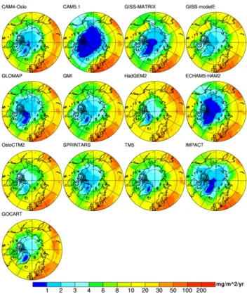
Fig. 1. Observed and modeled black carbon (BC) in snow concentrations in the Arctic. From left to right are ob-served BC-in-snow concentrations from Doherty et al. (2010), simulated concentrations over the observational domain from AeroCom Phase I models with inefficient meltwater scavenging (Ph I(IS)) and efficient scaveng-ing (Ph I(ES)), and simulated concentrations from Phase II models with inefficient scavengscaveng-ing (Ph II(IS)) and efficient scavenging (Ph II(ES)). The gray box indicates the 25% and 75% quartiles of the observations, and the

whisker depicts the full extent of the observations. Note that the maximum value of 783.5 ng g−1_{is outside the}

figure. The bold horizontal line shows the mean of the observations and models for each scenario. Each colored dot represents the mean of a particular model’s simulated BC-in-snow concentration averaged over grid cells matching the location, time, and depth of measurements.

1 5 10 50 100 200 1 5 10 50 100 200 Observed BC Concentration (ng/g)

Simulated BC Concentration [Ph I (IS)] (ng/g)

Arc. Ocean Ca. Arctic Alaska Ca. Sub−Arc. Greenland Ny−Alesund Tromso Russia DLR GISS LOA LSCE MATCH MPI−HAM TM5 UIO−CTM UIO−GCM UIO−GCM−V2 ULAQ UMI 1 5 10 50 100 200 1 5 10 50 100 200 Observed BC Concentration (ng/g)

Simulated BC Concentration [Ph I (ES)] (ng/g)

Arc. Ocean Ca. Arctic Alaska Ca. Sub−Arc. Greenland Ny−Alesund Tromso Russia DLR GISS LOA LSCE MATCH MPI−HAM TM5 UIO−CTM UIO−GCM UIO−GCM−V2 ULAQ UMI

Fig. 2. Log-scale scatter plot of BC-in-snow concentrations simulated in different regions with Phase I models applying inefficient meltwater scavenging (left) and efficient scavenging (right), compared with observations. The mean values for each region are averaged over grid cells matching the location, time, and depth of mea-surements.

26

Fig. 1. Observed and modeled black carbon (BC) in snow concen-trations in the Arctic. From left to right are observed BC-in-snow concentrations from Doherty et al. (2010), simulated concentrations over the observational domain from AeroCom phase I models with inefficient meltwater scavenging (Ph I(IS)) and efficient scaveng-ing (Ph I(ES)), and simulated concentrations from phase II models with inefficient scavenging (Ph II(IS)) and efficient scavenging (Ph II(ES)). The gray box indicates the 25 % and 75 % quartiles of the observations, and the whisker depicts the full extent of the

obser-vations. Note that the maximum value of 783.5 ng g−1 is outside

the figure. The bold horizontal line shows the mean of the observa-tions and models for each scenario. Each colored dot represents the mean of a particular model’s simulated BC-in-snow concentration averaged over grid cells matching the location, time, and depth of measurements.

and depth and were within the same grid cell in the model, we first averaged them and then treated them as one for the model comparison. Measurements collected in 1998 for the SHEBA campaign were not used in this exercise. Six mea-surements aligned with model grid cells that did not have any snow during the month of measurement, and were dis-carded from the analysis. After the merge and elimination, there were 485 unique observations in 8 regions. The follow-ing analysis is based on this merged sample set.

Data from Doherty et al. (2010) include most top and bot-tom depths from which the snow samples were taken, and we used this information to determine the appropriate model snow layer(s) to compare with. CLM uses up to 5 snow layers, depending on total snow thickness, so we weighted the BC concentration from each snow layer based on its fractional overlap with the measurement. If the sample only spanned a fraction of the snow layer thickness, we used this fraction multiplied by the snow mass in the layer as the weight for that layer. If the model layer was completely con-tained within the measurement boundaries, we used the total snow mass as the weight for that layer. Finally, the BC-in-snow concentrations from the available layers were averaged by the snow mass weights (normalized to 1) to get the model

(6)

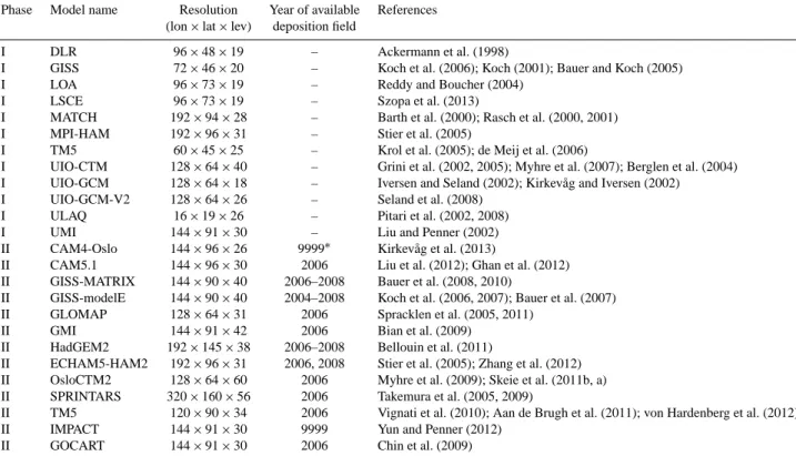
Table 1. Phase I and phase II AeroCom models used in this study.

Phase Model name Resolution Year of available References

(lon × lat × lev) deposition field

I DLR 96 × 48 × 19 – Ackermann et al. (1998)

I GISS 72 × 46 × 20 – Koch et al. (2006); Koch (2001); Bauer and Koch (2005)

I LOA 96 × 73 × 19 – Reddy and Boucher (2004)

I LSCE 96 × 73 × 19 – Szopa et al. (2013)

I MATCH 192 × 94 × 28 – Barth et al. (2000); Rasch et al. (2000, 2001)

I MPI-HAM 192 × 96 × 31 – Stier et al. (2005)

I TM5 60 × 45 × 25 – Krol et al. (2005); de Meij et al. (2006)

I UIO-CTM 128 × 64 × 40 – Grini et al. (2002, 2005); Myhre et al. (2007); Berglen et al. (2004)

I UIO-GCM 128 × 64 × 18 – Iversen and Seland (2002); Kirkevåg and Iversen (2002)

I UIO-GCM-V2 128 × 64 × 26 – Seland et al. (2008)

I ULAQ 16 × 19 × 26 – Pitari et al. (2002, 2008)

I UMI 144 × 91 × 30 – Liu and Penner (2002)

II CAM4-Oslo 144 × 96 × 26 9999∗ Kirkevåg et al. (2013)

II CAM5.1 144 × 96 × 30 2006 Liu et al. (2012); Ghan et al. (2012)

II GISS-MATRIX 144 × 90 × 40 2006–2008 Bauer et al. (2008, 2010)

II GISS-modelE 144 × 90 × 40 2004–2008 Koch et al. (2006, 2007); Bauer et al. (2007)

II GLOMAP 128 × 64 × 31 2006 Spracklen et al. (2005, 2011)

II GMI 144 × 91 × 42 2006 Bian et al. (2009)

II HadGEM2 192 × 145 × 38 2006–2008 Bellouin et al. (2011)

II ECHAM5-HAM2 192 × 96 × 31 2006, 2008 Stier et al. (2005); Zhang et al. (2012)

II OsloCTM2 128 × 64 × 60 2006 Myhre et al. (2009); Skeie et al. (2011b, a)

II SPRINTARS 320 × 160 × 56 2006 Takemura et al. (2005, 2009)

II TM5 120 × 90 × 34 2006 Vignati et al. (2010); Aan de Brugh et al. (2011); von Hardenberg et al. (2012)

II IMPACT 144 × 91 × 30 9999 Yun and Penner (2012)

II GOCART 144 × 91 × 30 2006 Chin et al. (2009)

∗_{Year “9999” indicates the deposition fields are generated from generic present-day meteorological conditions}

simulated BC concentrations for depths matching the posi-tion of the observaposi-tion. Due to the short spin-up time (1 year), BC concentrations in the deepest snow layer did not always reach equilibrium, especially in regions of perennial snow cover and low accumulation like Greenland. Thus, we only used the top 4 layers for the comparison. The CICE model applies 2 snow layers overlying 4 sea ice layers. The depth of the surface snow layer changes with the total snow thickness, equaling half of the total thickness when snow depth is less than or equal to 8 cm, and equaling 4 cm when the total snow depth is greater than 8 cm. For the observations sampled over sea ice, we used the top and bottom depth of the sample to determine which snow layer on sea ice should be compared with. If the sample extended to both layers, we used the aver-aged BC concentration from both layers to compare with the observation.

4 Results and discussion

4.1 Comparison of models and observations

Figure 1 shows BC-in-snow concentrations from models and observations. The spatial and temporal mean observed BC concentration averaged over all samples is 19.2 ng g−1. The 75 % quartile of the observations is close to the mean value due to skewness caused by high BC concentrations in some parts of Russia. Each color symbol in the figure represents

the mean BC concentration of a model simulation averaged over the locations (grid cell and layer) and months matching the observations. With inefficient melt scavenging (IS), the multi-model mean concentration over the observational

do-main is 14.8 ng g−1 for the twelve phase I simulations and

23.3 ng g−1for the thirteen phase II models. With efficient scavenging (ES), the phase I and phase II multi-model means are 14.0 and 22.3 ng g−1, respectively. The relatively small decrease associated with ES is discussed further in Sect. 4.4. There is a factor of 5 spread between the highest and lowest phase I model means, and a 6.5-fold spread among phase II models. The normalized standard deviation of model means is 0.41 and 0.40 for phase I and phase II IS runs, respectively. The inter-model variation in bias is also large for both phase I and phase II models (Table 2).

Three general factors could lead to the large inter-model diversity. Firstly, the transport schemes and meteorology vary between models. A large portion of the aerosol burden in the Arctic is transported from middle and lower latitudes (Koch and Hansen, 2005), amplifying the effects of differ-ences in model transport and removal physics. There are sev-eral pathways for pollutant transport to the Arctic, each with seasonality governed by scavenging efficiency and features of the Arctic dome. Stohl (2006) found that Arctic pollu-tion originating from North America and Asia generally ex-periences uplift outside the Arctic and then a descent into the Arctic. Pollution from Europe travels to the Arctic by

(7)

2404 C. Jiao et al.: Black carbon in Arctic snow assessment Table 2. Statistics of the comparison between models and observations. The correlation coefficients and significance levels are calculated by a linear regression fitted to all pairs of observations and corresponding modeled values from the same time and location. Biases are the

differences between the mean of modeled values and the mean of observations. The mean observed BC-in-snow concentration is 19.2 ng g−1.

Phase Model Correlation Bias (ng g−1) Correlation Bias (ng g−1)

coefficient coefficient

(inefficient scavenging) (efficient scavenging)

I DLR 0.21∗ −0.5 0.20∗ −1.3 I GISS 0.15∗ −7.0 0.14∗ −7.6 I LOA 0.15∗ −3.1 0.14∗ −4.0 I LSCE 0.16∗ −3.9 0.15∗ −4.8 I MATCH 0.11∗ −4.7 0.12∗ −5.8 I MPI-HAM 0.22∗ −13.2 0.21∗ −13.4 I TM5 0.28∗ −2.0 0.27∗ −2.7 I UIO-CTM 0.28∗ −8.7 0.27∗ −9.2 I UIO-GCM 0.15∗ −9.6 0.14∗ −10.0 I UIO-GCM-V2 0.14∗ −8.3 0.13∗ −8.8 I ULAQ 0.14∗ +10.7 0.14∗ +9.1 I UMI 0.21∗ −2.6 0.21∗ −3.6 Phase I mean – −4.4 – −5.2 II CAM4-Oslo 0.12∗ −0.2 0.12∗ −1.2 II CAM5.1 0.23∗ −13.0 0.22∗ −13.3 II GISS-MATRIX 0.21∗ −2.8 0.21∗ −3.4 II GISS-modelE 0.21∗ +7.8 0.20∗ +6.7 II GLOMAP 0.05 −0.8 0.04 −1.4 II GMI 0.10∗ +1.9 0.10∗ +0.8 II HadGEM2 0.18∗ +18.7 0.18∗ +17.3 II ECHAM5-HAM2 0.18∗ -4.9 0.17∗ −5.5 II OsloCTM2 0.10∗ +21.4 0.09∗ +19.5 II SPRINTARS 0.06 +5.3 0.06 +4.2 II TM5 0.14∗ +9.3 0.14∗ +8.1 II IMPACT 0.18∗ +3.8 0.17∗ +2.9 II GOCART 0.04 +7.3 0.03 +5.9 Phase II mean – +4.1 – +3.1

∗_{Indicates the regression is significant at α = 0.05 level.}

level transport followed by ascent into the Arctic or low-level transport alone. Secondly, the characteristics of aerosol deposition processes vary considerably between models. De-position fluxes are influenced by dry and wet removal rep-resentations, model precipitation, aerosol aging and mixing, and aerosol–cloud interactions. Among phase I models, the normalized standard deviation for Arctic BC deposition flux is 0.22 while for phase II models it is 0.27, indicating larger inter-model diversity for phase II contributions. Some of the increased spread in phase II BC deposition originates from use of different emission inventories, the third factor con-tributing to inter-model diversity.

Scatter plots shown in Figs. 2 and 3 compare simulated and observed BC concentrations in different regions. In gen-eral, observations and models are more likely to agree with each other in the Arctic Ocean and Ny-Ålesund. Models tend to overestimate BC-in-snow concentrations in the

cat-egories of Canadian Arctic, Alaska, Canadian Sub-Arctic and Greenland. In the Canadian Arctic, Canadian Sub-Arctic and Greenland, the means of phase I models are generally within a factor of 3 higher than the means of the observa-tions, while the means of phase II models are about a factor of 3–4 higher. In those three regions, the biases are positive for most of the models, although several models simulate BC concentrations relatively close to the observations. In Alaska, the model–observation disagreement is more substantial. The mean observed BC concentration in this region is about 12 ng g−1, while the highest value among all models is nearly 170 ng g−1, and the mean phase I and phase II concentrations are 50 ng g−1and 90 ng g−1, respectively. These model val-ues are higher than those of other regions (Figs. 2 and 3). Importantly, however, there are only 3 measurement samples in the Alaska region, all showing less than 20 ng g−1, poten-tially biasing the evaluation for this region. The multi-model

(8)

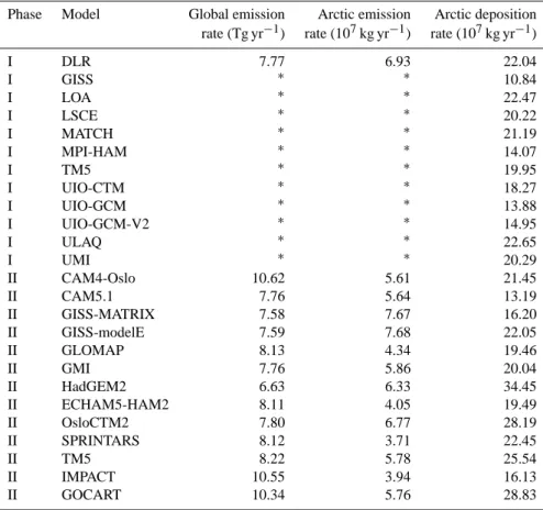
Table 3. Annual mean BC emission and deposition fluxes for the globe and Arctic (60◦N to 90◦N).

Phase Model Global emission Arctic emission Arctic deposition

rate (Tg yr−1) rate (107kg yr−1) rate (107kg yr−1)

I DLR 7.77 6.93 22.04 I GISS ∗ ∗ 10.84 I LOA ∗ ∗ 22.47 I LSCE ∗ ∗ 20.22 I MATCH ∗ ∗ 21.19 I MPI-HAM ∗ ∗ 14.07 I TM5 ∗ ∗ 19.95 I UIO-CTM ∗ ∗ 18.27 I UIO-GCM ∗ ∗ 13.88 I UIO-GCM-V2 ∗ ∗ 14.95 I ULAQ ∗ ∗ 22.65 I UMI ∗ ∗ 20.29 II CAM4-Oslo 10.62 5.61 21.45 II CAM5.1 7.76 5.64 13.19 II GISS-MATRIX 7.58 7.67 16.20 II GISS-modelE 7.59 7.68 22.05 II GLOMAP 8.13 4.34 19.46 II GMI 7.76 5.86 20.04 II HadGEM2 6.63 6.33 34.45 II ECHAM5-HAM2 8.11 4.05 19.49 II OsloCTM2 7.80 6.77 28.19 II SPRINTARS 8.12 3.71 22.45 II TM5 8.22 5.78 25.54 II IMPACT 10.55 3.94 16.13 II GOCART 10.34 5.76 28.83

∗_{The total amounts of BC emission are the same for phase I models.}

mean concentration of BC in surface snow, averaged annu-ally over all of Alaska, is 41 ng g−1_{, smaller than averages}

over the Alaskan sampling domain. In Tromsø and Rus-sia, models tend to underestimate BC-in-snow concentra-tions over the observational domain. The mean for phase I models is around half the observational mean. The phase II mean is closer to the observations, though these models show more inter-model diversity in these regions than phase I mod-els. One potential factor that could contribute to the underes-timation of BC-in-snow concentration in Russia is the omis-sion of high-latitude flaring source in the AeroCom emisomis-sion inventories (Stohl et al., 2013).

From Figs. 2 and 3, we see that the models capture some spatial characteristics of the observed BC-in-snow concen-trations, though correlations between the observations and models are weak. This indicates that the current stage of global aerosol models has difficulty in reproducing the ob-served distribution of BC in Arctic snow, caused by some combination of biased emission inventories, atmospheric and/or snow aerosol parametrizations, or inconsistent mete-orology from that which prevailed during the measurement campaign. Table 2 shows the correlation coefficient (R), sta-tistical significance (i.e., p value smaller than 0.05), and bias between the models and observations. The correlation

co-efficients are generally small, ranging from 0.11 to 0.28 in phase I IS simulations and 0.12 to 0.27 in ES simulations. In phase II, the correlation coefficients range from 0.04 to 0.23 and 0.03 to 0.22, respectively, in IS and ES simula-tions. Despite poor correlation coefficients, mean model bi-ases are reasonably small. Phase I models generally slightly underestimate observed Arctic BC-in-snow concentrations (Table 2). This is consistent with results from Koch et al. (2009), showing that most AeroCom phase I models under-estimate the atmospheric concentration of BC compared with observations in the remote Arctic, and also with Shindell et al. (2008), who showed that HTAP models also generally underestimate near-surface measurements of BC at the Arc-tic Alaska locations Barrow and Alert. Five of the phase II models are biased low while the other eight overestimate BC-in-snow concentrations. With inefficient scavenging, the

bi-ases range from −13.2 ng g−1 _{to +10.7 ng g}−1 _{for phase I}

models. For phase II, the lowest and highest mean biases are −13.0 ng g−1and +21.4 ng g−1.

We have so far reported results for both inefficient (IS) and efficient (ES) melt scavenging parameters. The IS pa-rameters are derived from a very limited set of observations, while the ES studies are idealized and designed to test the sensitivity of results to this parameter. Although there is large

(9)

2406 C. Jiao et al.: Black carbon in Arctic snow assessment

Obs. Ph I(IS) Ph I(ES) Ph II(IS) Ph II(ES)

0 10 20 30 40 50

Fig. 1. Observed and modeled black carbon (BC) in snow concentrations in the Arctic. From left to right are ob-served BC-in-snow concentrations from Doherty et al. (2010), simulated concentrations over the observational domain from AeroCom Phase I models with inefficient meltwater scavenging (Ph I(IS)) and efficient scaveng-ing (Ph I(ES)), and simulated concentrations from Phase II models with inefficient scavengscaveng-ing (Ph II(IS)) and efficient scavenging (Ph II(ES)). The gray box indicates the 25% and 75% quartiles of the observations, and the

whisker depicts the full extent of the observations. Note that the maximum value of 783.5 ng g−1_{is outside the}

figure. The bold horizontal line shows the mean of the observations and models for each scenario. Each colored dot represents the mean of a particular model’s simulated BC-in-snow concentration averaged over grid cells matching the location, time, and depth of measurements.

Simulated BC Concentration [Ph I (IS)] (ng/g)

Arc. Ocean Ca. Arctic Alaska Ca. Sub−Arc. Greenland Ny−Alesund Tromso Russia DLR GISS LOA LSCE MATCH MPI−HAM TM5 UIO−CTM UIO−GCM UIO−GCM−V2 ULAQ UMI 1 5 10 50 100 200 1 5 10 50 100 200 Observed BC Concentration (ng/g)

Simulated BC Concentration [Ph I (ES)] (ng/g)

Arc. Ocean Ca. Arctic Alaska Ca. Sub−Arc. Greenland Ny−Alesund Tromso Russia DLR GISS LOA LSCE MATCH MPI−HAM TM5 UIO−CTM UIO−GCM UIO−GCM−V2 ULAQ UMI

Fig. 2. Log-scale scatter plot of BC-in-snow concentrations simulated in different regions with Phase I models applying inefficient meltwater scavenging (left) and efficient scavenging (right), compared with observations. The mean values for each region are averaged over grid cells matching the location, time, and depth of mea-surements.

26

Fig. 2. Log-scale scatter plot of BC-in-snow concentrations simulated in different regions with phase I models applying inefficient meltwater scavenging (left panel) and efficient scavenging (right panel), compared with observations. The mean values for each region are averaged over grid cells matching the location, time, and depth of measurements.

Simulated BC Concentration [Ph II (IS)] (ng/g)

Arc. Ocean Ca. Arctic Alaska Ca. Sub−Arc. Greenland Ny−Alesund Tromso Russia CAM4−Oslo CAM5.1 GISS−MATRIX GISS−modelE GLOMAP GMI HadGEM2 ECHAM5−HAM2 OsloCTM2 SPRINTARS TM5 IMPACT GOCART 1 5 10 50 100 200 1 5 10 50 100 200 Observed BC Concentration (ng/g)

Simulated BC Concentration [Ph II (ES)] (ng/g)

Arc. Ocean Ca. Arctic Alaska Ca. Sub−Arc. Greenland Ny−Alesund Tromso Russia CAM4−Oslo CAM5.1 GISS−MATRIX GISS−modelE GLOMAP GMI HadGEM2 ECHAM5−HAM2 OsloCTM2 SPRINTARS TM5 IMPACT GOCART

Fig. 3. Same as Figure 2, but for Phase II models.

Fig. 4. Relationships between simulated BC-in-snow concentrations averaged over the locations and months of observations and over the whole Arctic region. The abscissa is the surface layer BC-in-snow concentration averaged over grid cells matching the location and time of measurements. The ordinate is the annual mean

surface layer BC-in-snow concentration averaged over the whole Arctic region (60◦_{N to 90}◦_{N) (left), and}

averaged over the Arctic with insolation weighting (right).

27 Fig. 3. Same as Fig. 2, but for phase II models.

uncertainty in melt scavenging efficiency, a growing number of observational studies indicate that BC is scavenged ineffi-ciently with melt water (Xu et al., 2012; Doherty et al., 2013; Sterle et al., 2013). From field measurements, Doherty et al. (2013) derived BC meltwater scavenging efficiencies ranging from 10 % to 30 %, broadly consistent with the parameters used by Flanner et al. (2007). We also find that 16 of 25 Ae-roCom simulations produce a higher correlation coefficient with IS than ES (though the mean improvement is only 0.01). Consequently, the analysis that follows focuses on IS simu-lations, except for a sensitivity analysis of melt scavenging in Sect. 4.4.

The observations cover a large area of the Arctic but are relatively sparse in some sectors. Also, the measurements were conducted only during spring and summer, the sea-sons of most relevance for radiative effects. Thus, the ques-tion arises of how well the sampling domain represents the Arctic-mean distribution of BC in surface snow. Figure 4a shows, for each model, the annual mean BC concentration in the surface snow layer averaged over the whole Arctic plot-ted against the annual mean surface-layer BC concentration

averaged spatially and temporally over the model domain matching observations. There is a strong linear relationship between these two quantities. The R2of the linear fit is 0.73 and statistically significant at the 0.001 level. Figure 4b plots BC concentrations weighted by the surface incident solar ra-diation (ISR) and averaged over the whole Arctic against the same quantity on the x axis as Fig. 4a. This metric places a stronger weight on polluted snow exposed to intense sun-light, which exerts a stronger radiative effect than the same snow surface in polar darkness. It thus gives a better indi-cation of how representative the measurement survey is of the Arctic BC-in-snow radiative effect. The linear

relation-ship in Fig. 4b is stronger, with a R2 value of 0.80. This

result suggests that the sampling domain surveyed by Do-herty et al. (2010), conducted during seasons of relatively strong insolation, could provide a reasonable constraint on Arctic-wide annual-mean radiative effects from BC-in-snow. The correlation between annual-mean BC concentrations at each of the measurement sites (a proxy for a scenario with year-round sampling) and Arctic-mean BC-in-snow concen-trations is very high (R2=0.95; not shown).

(10)

Fig. 4. Relationships between simulated BC-in-snow concentrations averaged over the locations and months of observations and over the whole Arctic region. The abscissa is the surface layer BC-in-snow concentration averaged over grid cells matching the location and time of

measurements. The ordinate is the annual mean surface layer BC-in-snow concentration averaged over the whole Arctic region (60◦N to

90◦N) (left panel: Fig. 4a), and averaged over the Arctic with insolation weighting (right panel: Fig. 4b).

−900 −60 −30 0 30 60 90

30 60 90 120

Latitude (Degree North)

Black Carbon Emission Flux (mg/m

2/yr) 50 60 70 80 90 0 10 20 30 40

2/yr) Phase I CAM4−Oslo CAM5.1 GISS−MATRIX GISS−modelE GLOMAP GMI HadGEM2 ECHAM5−HAM2 OsloCTM2 SPRINTARS TM5 IMPACT GOCART

Fig. 5. Annual, zonal-mean black carbon emission fluxes applied in Phase I and Phase II models for the global (left) and in more detail in the northern latitude (right) regions.

−900 −60 −30 0 30 60 90 10 20 30 40 50

Black Carbon Deposition Flux (mg/m

2/yr) DLR GISS LOA LSCE MATCH MPI−HAM TM5 UIO−CTM UIO−GCM UIO−GCM−V2 ULAQ UMI −900 −60 −30 0 30 60 90 20 40 60 80

2/yr) CAM4−Oslo CAM5.1 GISS−MATRIX GISS−modelE GLOMAP GMI HadGEM2 ECHAM5−HAM2 OsloCTM2 SPRINTARS TM5 IMPACT GOCART

Fig. 6. Annual, zonal-mean black carbon deposition fluxes for Phase I (left) and Phase II (right) models. (Note the scale on ordinate is different for the two plots.)

28

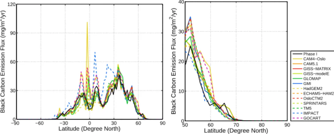
Fig. 5. Annual, zonal-mean black carbon emission fluxes applied in phase I and phase II models for the global (left panel: Fig. 5a) and in more detail in the northern latitude (right panel: Fig. 5b) regions.

4.2 Emissions

Phase I models apply the same emission inventory, while phase II models use different inventories. Figure 5 shows the zonal-mean emissions used in each model, plotted globally and for the northern high latitudes. From Fig. 5 we see that phase II models show substantial variations in emissions, es-pecially in the tropics, where biomass burning emissions are large and more variable between inventories. The peak

emis-sion fluxes are mostly within 30–40◦N, which includes major

populated industrial regions (East Asia, South Asia, parts of North America and Europe). Figure 5b shows that the inter-model variation in BC emissions at high latitudes is relatively small, and that emissions north of 70◦N are negligible in the inventories applied.

To identify the importance of inter-model variability in

lo-cal emissions, we regress annual mean Arctic (60–90◦N)

sur-face BC-in-snow concentrations against annual-mean emis-sion fluxes, but find insignificant correlations both with the

fluxes averaged over the Arctic (60–90◦N) (R2=0.03, p =

0.55) and with emission fluxes averaged in a larger region

(50–90◦N) (R2=0.09, p = 0.29). Among phase II models,

the ratio between annual mean Arctic deposition and Arctic emission ranges from 2.1 to 6.1, with 10 models having a ra-tio larger than 3. For phase I models, the rara-tio ranges from 1.6 to 3.3. This proves, as expected, that most of the model BC depositing in the Arctic originates from emissions out-side the Arctic. The large range of this ratio reveals poten-tial large inter-model vertical variability in aerosol scaveng-ing efficiency as well as in transport efficiency to the Arctic. Variability in mid- and low-latitude emissions contributes to some of the diversity in Arctic deposition of phase II models, but is entwined with the effects of variation in model trans-port and scavenging mechanisms.

4.3 Inter-model deposition variability

Inter-model variability in BC deposition, the primary direct driver of variation in BC-in-snow concentrations, originates from different emissions and model physics. Figure 6 shows

(11)

2408 C. Jiao et al.: Black carbon in Arctic snow assessment −900 −60 −30 0 30 60 90 30 60 90 120

2/yr) 50 60 70 80 90 0 10 20 30 40

2/yr) Phase I CAM4−Oslo CAM5.1 GISS−MATRIX GISS−modelE GLOMAP GMI HadGEM2 ECHAM5−HAM2 OsloCTM2 SPRINTARS TM5 IMPACT GOCART

Fig. 5. Annual, zonal-mean black carbon emission fluxes applied in Phase I and Phase II models for the global (left) and in more detail in the northern latitude (right) regions.

−900 −60 −30 0 30 60 90 10 20 30 40 50

2/yr) DLR GISS LOA LSCE MATCH MPI−HAM TM5 UIO−CTM UIO−GCM UIO−GCM−V2 ULAQ UMI −900 −60 −30 0 30 60 90 20 40 60 80

Fig. 6. Annual, zonal-mean black carbon deposition fluxes for Phase I (left) and Phase II (right) models. (Note the scale on ordinate is different for the two plots.)

28

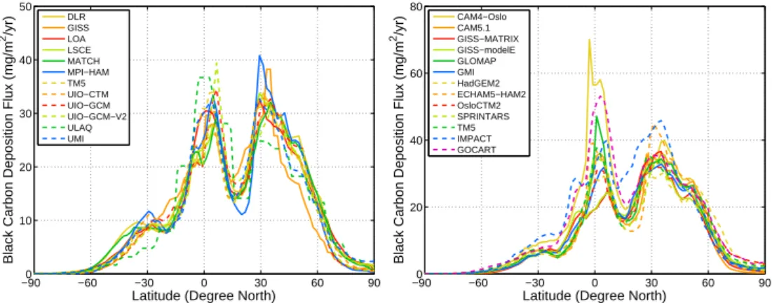
Fig. 6. Annual, zonal-mean black carbon deposition fluxes for phase I (left panel) and phase II (right panel) models. (Note the scale on ordinate is different for the two plots.)

annual zonal-mean BC deposition for phase I (left panel) and phase II (right panel) models, and indicates that the inter-model variation is generally larger in phase II inter-models, in-cluding at northern high latitudes. The peak deposition fluxes

are near the Equator and 30–40◦N, owing to large emissions

sources at these latitudes and efficient removal from ITCZ and monsoon precipitation. Spatial distributions of annual

mean BC deposition over 50–90◦_{N are shown in Figs. 7 and}

8. These figures show similar patterns among the models, with relatively large deposition over Northern Europe, North America and East Asia, and small deposition over Green-land and the Arctic Ocean. Though the spatial patterns are consistent among these models, the relative magnitudes are different. The phase II HadGEM2 and OsloCTM2 models, in particular, show large BC deposition fluxes in the Arctic. The

strong linear relationship (R2=0.80, p < 0.001) between

BC deposition fluxes averaged over 60–90◦N and surface

layer BC-in-snow concentration averaged over the same re-gion demonstrates the first-order importance of rere-gional de-position fluxes.

The normalized standard deviation of Arctic deposition is 0.22 for phase I and 0.27 for phase II models. While there is no inter-model variation of emissions (in terms of total emit-ted mass) for phase I models, the normalized standard devia-tion of phase II Arctic emissions is 0.23 (Table 3). Together, these results imply that aerosol transport, evolution, and re-moval processes (combined) are more important contributors to inter-model variation in Arctic BC deposition than emis-sions. This is also consistent with previous AeroCom analy-ses showing large variability in model aerosol burdens with harmonized emissions (Textor et al., 2007).

The seasonal cycle of BC deposition can be important for Arctic BC-in-snow radiative effects. Forcing only occurs dur-ing the sunlit period, but BC deposited durdur-ing winter can be-come exposed at the surface during spring and summer melt. Figure 9 shows the monthly mean BC deposition fluxes

av-eraged over 60–90◦_{N for phase I and phase II models. The}

Arctic BC deposition fluxes are relatively low during winter,

Fig. 7. Annual mean black carbon deposition fluxes for phase I

models, plotted from 50◦N to 90◦N.

when precipitation rates are low and the atmosphere is sta-bly stratified. Deposition starts to increase after March and models generally show a sharp peak between June and Au-gust. Among phase I models, one shows Arctic BC depo-sition peaks in June, seven peak in July, and four in August. Among phase II models, one peaks in May, nine peak in July, one in August and two in September. The seasonal cycles of deposition among phase I models are broadly similar. Most phase II models follow similar seasonal patterns as phase I, though some models peak later. For some models, the con-trast between summer and winter is high, while for others it is not. For example, the Arctic deposition flux in July is at least a factor of 3 higher than that in the lowest month for phase II CAM4-Oslo and HadGEM2 models, while seasonal variation is very small in the GMI and IMPACT models. This

(12)

Fig. 8. Annual mean black carbon deposition fluxes for phase II

models, plotted from 50◦N to 90◦N.

diversity originates both from different emission inventories and different chemical and physical parametrizations. Most AeroCom models do not have seasonality for fossil fuel and biofuel emissions. In reality, however, high-latitude biofuel and fossil fuel emission sources tend to be stronger in winter, indicating a potential bias in seasonality of deposition fluxes simulated with seasonally constant emission inventories.

Dividing the Arctic BC column burden by the Arctic de-position flux provides a proxy for Arctic BC residence time. This is imperfect because BC passing through the Arctic at-mosphere will contribute to mean burden but not deposition. Nonetheless, the averages are taken over a sufficiently large area so that they should approximate actual Arctic residence time. Here, for simplification, we will call this term “Arc-tic residence time” despite its potential bias. The Arc“Arc-tic resi-dence time is an indicator of how effectively BC in the Arctic atmosphere deposits through wet and dry processes. Textor et al. (2006) reported that global BC atmospheric residence times for phase I models ranges from 5.2 to 15.0 days. Fig-ure 10 shows the global and Arctic atmospheric residence times of BC in phase II models. The global BC residence time ranges from 3.9 to 11.9 days while the Arctic residence time ranges from 3.7 to 23.2 days. The Arctic residence time is longer on average by 4.0 days (median of 2.5 days) than the global residence time, although three models show shorter Arctic than global residence times. Causes for high Arctic residence times include low precipitation rates (especially

during polar winter), stable stratification that limits dry tur-bulent deposition, and long residence time of air parcels that become trapped within the polar dome. Koch et al. (2009) evaluated Arctic atmospheric BC in AeroCom phase I mod-els and found that increasing BC lifetime, which is accom-plished by decreasing the aging rate or by reducing removal by ice clouds, has a large impact on BC surface concentra-tions in remote regions. Analysis of surface measurements at Barrow, Alaska, indicates that the seasonal cycle of “Arc-tic haze” is dominated by wet scavenging rather than effi-ciency of transport pathways from source regions (Garrett et al., 2010; Browse et al., 2012; Lund and Berntsen, 2012; Wang et al., 2013). Liu et al. (2011) concluded that the simu-lation of BC in the Arctic is significantly improved by using a parameterization of BC aging rate that is proportional to the OH radical concentration, reducing dry deposition veloc-ities over ice and snow, and decreasing ice cloud wet removal efficiency. These changes increased wintertime BC concen-trations by a factor of 50–100. Browse et al. (2012) improved the simulated seasonal cycle of Arctic aerosols by including more realistic treatment of the transition in scavenging effi-ciency associated with changes in cloud phases. von Hard-enberg et al. (2012) reported a more realistic yearly averaged simulated AOD in the Arctic compared to observations by us-ing the modified wet scavengus-ing scheme suggested by Bour-geois and Bey (2011). Together, these studies indicate that deposition parametrizations are critical for determining both the latitudinal profile of the modeled BC and the efficiency through which Arctic atmospheric BC is removed. Precise attribution of how physical parameterizations contribute to model diversity requires carefully designed perturbation ex-periments, such as those conducted by Lee et al. (2013a).

One consequence of our methodology for simulating BC-in-snow concentrations is that the meteorological conditions used to drive CLM and CICE may be inconsistent with those determining the model deposition amounts. We chose to drive each simulation with the same 2005–2009 reanalysis data because (1) these meteorological conditions are likely to be more compatible than model-generated fields with condi-tions that prevailed during the measurement campaigns, and thus will produce more similar model snowpack conditions to those from which measurements were drawn, and (2) us-ing the same meteorological conditions for each simulation reduces the number of free variables and enables a more lu-cid intercomparison of BC-in-snow concentrations resulting from different BC deposition fields. To evaluate the potential impact of this design choice, we conducted a sensitivity study with CLM and CICE coupled interactively (online) with the Community Atmosphere Model (CAM), and the transport and deposition of aerosols simulated prognostically in a self-consistent way with model meteorology. We then used depo-sition fields from this simulation to drive CLM and CICE of-fline in the same period, using the same reanalysis product as described in Sect. 3. We found that the model–measurement

bias averaged over the sampling domain is −9.7 ng g−1 in

(13)

2410 C. Jiao et al.: Black carbon in Arctic snow assessment J F M A M J J A S O N D 0 3 6 9 12 15 Month

2/yr) DLR GISS LOA LSCE MATCH MPI−HAM TM5 UIO−CTM UIO−GCM UIO−GCM−V2 ULAQ UMI J F M A M J J A S O N D 0 5 10 15 20 25 Month

Fig. 9. Seasonal cycle of black carbon deposition fluxes averaged over the Arctic (60◦_{N to 90}◦_{N) for Phase I}

(left) and Phase II (right) models. (Note the scale on ordinate is different for the two plots.)

0 5 10 15 20 25

BC Residence Time (Day)

N/A N/A N/A

CAM4−Oslo CAM5.1GISS−MATRIXGISS−modelE GLOMAP GMI HadGEM2

ECHAM5−HAM2 OsloCTM2 SPRINTARS TM5_IMPACT

GOCART Arctic Global

Fig. 10. Global and Arctic atmospheric residence times for black carbon in Phase II models. (Three models are excluded in this analysis due to missing or incomplete data.)

31

Fig. 9. Seasonal cycle of black carbon deposition fluxes averaged over the Arctic (60◦N to 90◦N) for phase I (left panel) and phase II (right

panel) models. (Note the scale on ordinate is different for the two plots.)

J F M A M J J A S O N D 0 3 6 9 12 15 Month

2/yr) DLR GISS LOA LSCE MATCH MPI−HAM TM5 UIO−CTM UIO−GCM UIO−GCM−V2 ULAQ UMI J F M A M J J A S O N D 0 5 10 15 20 25 Month

Fig. 9. Seasonal cycle of black carbon deposition fluxes averaged over the Arctic (60◦_{N to 90}◦_{N) for Phase I}

(left) and Phase II (right) models. (Note the scale on ordinate is different for the two plots.)

0 5 10 15 20 25

BC Residence Time (Day)

N/A N/A N/A

CAM4−Oslo CAM5.1GISS−MATRIXGISS−modelE GLOMAP GMI HadGEM2

ECHAM5−HAM2 OsloCTM2 SPRINTARS TM5_IMPACT

GOCART Arctic Global

Fig. 10. Global and Arctic atmospheric residence times for black carbon in Phase II models. (Three models are excluded in this analysis due to missing or incomplete data.)

31

Fig. 10. Global and Arctic atmospheric residence times for black carbon in phase II models. (Three models are excluded in this anal-ysis due to missing or incomplete data.)

the online simulation, while it is −0.1 ng g−1 for the

of-fline CLM/CICE simulation. The correlation coefficient be-tween model and observation is 0.16 for online simulation and 0.18 for offline simulation. This sensitivity study indi-cates that choice of meteorology can have a significant im-pact on model–measurement comparison. The sign of imim-pact is also consistent with a preliminary study (Sarah Doherty, personal communication, 2013), suggesting that use of in-consistent deposition and precipitation fluxes can produce a high bias in surface layer BC concentrations. This could im-ply that model deposition fluxes in the Arctic have more low bias (or less high bias) than indicated by our study. Applying identical meteorological fields with all deposition fields also likely reduces inter-model diversity in simulated BC-in-snow amounts.

Table 4. Arctic BC-in-snow radiative effects, averaged from 60◦N

to 90◦N (W m−2). Phase I ISa ESb Phase II ISa ESb DLR 0.18 0.15 CAM4-Oslo 0.16 0.13 GISS 0.10 0.09 CAM5.1 0.06 0.05 LOA 0.17 0.14 GISS-MATRIX 0.12 0.10 LSCE 0.15 0.13 GISS-modelE 0.20 0.17 MATCH 0.14 0.12 GLOMAP 0.16 0.14 MPI-HAM 0.07 0.06 GMI 0.15 0.13 TM5 0.19 0.16 HadGEM2 0.28 0.24 UIO-CTM 0.13 0.11 ECHAM5-HAM2 0.11 0.09 UIO-GCM 0.10 0.08 OsloCTM2 0.27 0.23 UIO-GCM-V2 0.10 0.08 SPRINTARS 0.18 0.15 ULAQ 0.25 0.21 TM5 0.23 0.20 UMI 0.18 0.15 IMPACT 0.17 0.15 GOCART 0.22 0.18

a_{IS indicates inefficient meltwater scavenging.} b_{ES indicates efficient meltwater scavenging.}

4.4 The effect of meltwater scavenging

As insolation increases during spring in the Arctic, surface snow begins to melt. As the meltwater percolates into deeper snow, it collects some of the impurities, altering the verti-cal distribution of BC in snow and sea ice. We ran CLM and CICE with two sets of BC meltwater scavenging coeffi-cients in order to evaluate impacts of uncertainty in these pa-rameters. The inefficient scavenging (IS) scenario applies the same scavenging coefficients used by Flanner et al. (2007), leading to accumulation of BC near the snow surface as melt occurs, whereas the ES sensitivity studies apply scavenging coefficients of 1.0 for both hydrophilic and hydrophobic BC. Though the ES scenario is not supported with observations, it enables an assessment of the potential impact of this pa-rameter on the model evaluations.

Figure 11 divides the model–measurement comparison shown in Fig. 1 into eight different regions. From Fig. 11, we can see that the scavenging sensitivity study has different

(14)

Obs. Ph I(IS) Ph I(ES) Ph II(IS) Ph II(ES) 0 10 20 30 40

Arctic Ocean, Number of Obs. = 64

Obs. Ph I(IS) Ph I(ES) Ph II(IS) Ph II(ES) 0

10 20 30 40

Canadian Arctic, Number of Obs. = 118

50 100 150 200

Alaska, Number of Obs. = 3

30 60 90 120

Canada Sub−Arctic, Number of Obs. = 30

Obs. Ph I(IS) Ph I(ES) Ph II(IS) Ph II(ES) 0 5 10 15 20 25 30

Greenland, Number of Obs. = 84

10 20 30 40

Ny-˚Alesund, Numb er of Obs. = 26

Obs. Ph I(IS) Ph I(ES) Ph II(IS) Ph II(ES) 0 10 20 30 40 50

Tromsø, Numb er of Obs. = 20

20 40 60 80

Russia, Number of Obs. = 140

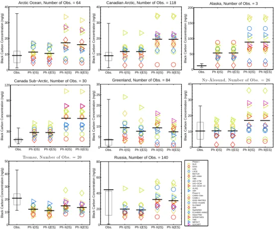
Fig. 11. Same as Figure 1, but plotted for 8 individual regions. The number of observations within each region

is listed in the figure titles.

32

Fig. 11. Same as Fig. 1, but plotted for 8 individual regions. The number of observations within each region is listed in the figure titles.

impacts in different regions, reflecting differing degrees to which the regional sampling domains are affected by melt. In some regions, including the Canadian Arctic, Alaska, Cana-dian Sub-Arctic and Ny-Ålesund, the differences between IS and ES scenarios are very small. In Greenland, however, and to a lesser extent Tromsø and the Arctic Ocean, there are no-ticeably higher modeled BC-in-snow concentrations in the IS scenario. To highlight the role of snowmelt in modulating the importance of these parameters, we plotted the histogram of the months when the samples were collected and the monthly mean snowmelt rate averaged over grid cells matching the observations in the different regions (Fig. 12). In regions that show no significant difference between IS and ES scenar-ios, there were few samples collected during times of large snowmelt. For example, the Ny-Ålesund samples were col-lected during March–May, before the July peak in model snowmelt rate, meaning the sub-sampled model domain is largely unaffected by melt. Most of the Greenland samples were collected at lower elevations during July and August, however, coincident with peak melt rates in the matching model domain (Fig. 12). About 43 % of the sampling space coincides with the top model snow layer, and over 70 % of it coincides with the top two model layers, where simulated concentrations are sensitive to the scavenging parameter dur-ing conditions of melt. Because much of the sampldur-ing space

does not coincide with strong melt, however, the melt scav-enging coefficients have only a second-order impact on the Arctic-wide model–measurement evaluation.

5 BC-in-snow radiative effect

Figure 13 shows the annual mean surface radiative effects caused by BC in snow, as simulated with deposition fields from the phase I and phase II models. Regions with rela-tively large radiative effects are northern Europe, Russia and Greenland. The two primary factors influencing annual-mean radiative effect in different regions are the amount of BC in snow and the seasonal evolution of snow cover fraction. For example, perennial snow cover in Greenland enables large forcing in this region despite relatively small BC concen-trations. Persistence of cryospheric cover through summer is especially important because it maximizes the amount of in-solation incident on impurity-laden snow and ice. The rela-tively small BC-in-snow radiative effects in central Green-land are caused by the small BC deposition fluxes in this area (Figs. 7 and 8) as well as little surface BC accumu-lation due to low snowmelt rate associated with high alti-tude and low temperature. Arctic annual mean BC in snow radiative effects for both phases and both sets of meltwater scavenging coefficients are shown in Table 4. With inefficient

(15)

2412 C. Jiao et al.: Black carbon in Arctic snow assessment J F M A M J J A S O N D 0 5 10 15 20 25 Number of Samples Month Arctic Ocean J F M A M J J A S O N D0 5 10 15 20 25

Snow and Top Ice Melt Rate (mm/day)

J F M A M J J A S O N D 0 50 100 Number of Samples Month Canadian Arctic J F M A M J J A S O N D0 2 4

Snow Melt Rate (mm/day)

J F M A M J J A S O N D 0 2 4 Number of Samples Month Alaska J F M A M J J A S O N D0 0.5 1

J F M A M J J A S O N D 0 5 10 15 20 25 30 Number of Samples Month Canada Sub−Arctic J F M A M J J A S O N D0 0.5 1 1.5 2 2.5 3

J F M A M J J A S O N D 0 50 100 Number of Samples Month Greenland J F M A M J J A S O N D0 2 4

J F M A M J J A S O N D 0 10 20 30 Number of Samples Month Ny-˚Alesund J F M A M J J A S O N D0 2 4 6

J F M A M J J A S O N D 0 5 10 Number of Samples Month Tromsø J F M A M J J A S O N D0 10 20

J F M A M J J A S O N D 0 50 100 150 Number of Samples Month Russia J F M A M J J A S O N D0 1 2 3

Fig. 12. Histogram of the months when the samples are collected in each regions (plotted against left axis) and

seasonal cycle of snow and ice melt rates (plotted against right axis). The melt rates are averaged only over grid cells containing observations within each region.

Fig. 13. Annual mean BC-in-snow radiative effects averaged across Phase I (left) and Phase II (right) models

with inefficient meltwater scavenging.

33

Fig. 12. Histogram of the months when the samples are collected in each region (plotted against left axis) and seasonal cycle of snow and ice melt rates (plotted against right axis). The melt rates are averaged only over grid cells containing observations within each region.

J F M A M J J A S O N D 0 5 10 15 20 25 Number of Samples Month Arctic Ocean J F M A M J J A S O N D0 5 10 15 20 25

Snow and Top Ice Melt Rate (mm/day)

J F M A M J J A S O N D 0 50 100 Number of Samples Month Canadian Arctic J F M A M J J A S O N D0 2 4

J F M A M J J A S O N D 0 2 4 Number of Samples Month Alaska J F M A M J J A S O N D0 0.5 1

J F M A M J J A S O N D 0 5 10 15 20 25 30 Number of Samples Month Canada Sub−Arctic J F M A M J J A S O N D0 0.5 1 1.5 2 2.5 3

J F M A M J J A S O N D 0 50 100 Number of Samples Month Greenland J F M A M J J A S O N D0 2 4

J F M A M J J A S O N D 0 10 20 30 Number of Samples Month Ny-˚Alesund J F M A M J J A S O N D0 2 4 6

J F M A M J J A S O N D 0 5 10 Number of Samples Month Tromsø J F M A M J J A S O N D0 10 20

J F M A M J J A S O N D 0 50 100 150 Number of Samples Month Russia J F M A M J J A S O N D0 1 2 3

Fig. 12. Histogram of the months when the samples are collected in each regions (plotted against left axis) and seasonal cycle of snow and ice melt rates (plotted against right axis). The melt rates are averaged only over grid cells containing observations within each region.

Fig. 13. Annual mean BC-in-snow radiative effects averaged across Phase I (left) and Phase II (right) models with inefficient meltwater scavenging.

33

Fig. 13. Annual mean BC-in-snow radiative effects averaged across phase I (left panel) and phase II (right panel) models with inefficient meltwater scavenging.

scavenging, the modeled Arctic radiative effects for phase I

models range from 0.07 W m−2 to 0.25 W m−2, and range

from 0.06 W m−2 to 0.28 W m−2for phase II models. With

efficient scavenging, the radiative effects are slightly smaller,

ranging from 0.06–0.21 W m−2 and 0.05–0.24 W m−2,

re-spectively, for phase I and phase II models.

The multi-model mean BC-in-snow radiative effect

aver-aged over the Arctic (here, 60–90◦_{N) is 0.15 W m}−2 _and

0.18 W m−2 _{for phase I and phase II models, respectively,}

with inefficient meltwater scavenging. Model biases in BC concentrations in snow may also translate into biases in Arctic-mean radiative effect. Here we used the ratio be-tween simulated and observed BC concentrations in different regions of the Arctic to derive observationally constrained forcings. In doing so, we assume a linear relationship be-tween the near surface BC-in-snow concentration and

radia-tive effect, which is a reasonable assumption for small per-turbations about low BC concentrations (e.g., Flanner et al., 2007), such as those found in most of the Arctic. We divided the Arctic into 6 regions (Europe, Russia, Alaska, Canada, Greenland and the Arctic Ocean) and scaled the modeled radiative effects in each region by the ratio of observed-to-modeled BC concentrations in the sampling domain within each region. For each of the five land-based regions, the ra-diative effect is simulated with CLM, whereas rara-diative ef-fect within the Arctic Ocean is simulated with CICE. Us-ing this correction technique, we calculated an Arctic-mean

BC-in-snow radiative effect of 0.17 W m−2for the combined

phase I and phase II ensembles. This approach has the ad-vantage of accounting for model performance in different re-gions of the Arctic, but is only useful to the extent that model