HAL Id: halshs-00585966
https://halshs.archives-ouvertes.fr/halshs-00585966
Preprint submitted on 14 Apr 2011
HAL is a multi-disciplinary open access archive for the deposit and dissemination of sci-entific research documents, whether they are pub-lished or not. The documents may come from teaching and research institutions in France or
L’archive ouverte pluridisciplinaire HAL, est destinée au dépôt et à la diffusion de documents scientifiques de niveau recherche, publiés ou non, émanant des établissements d’enseignement et de recherche français ou étrangers, des laboratoires
Agriculture and trade liberalization in Vietnam
Barbara Coello
To cite this version:
WORKING PAPER N° 2008 - 75
Agriculture and trade liberalization in Vietnam
Barbara Coello
JEL Codes: Q17, Q12, C21
Keywords: trade liberalization, agriculture, price
pass-through
P
ARIS-
JOURDANS
CIENCESE
CONOMIQUESL
ABORATOIRE D’E
CONOMIEA
PPLIQUÉE-
INRA 48,BD JOURDAN –E.N.S.–75014PARISTÉL. :33(0)143136300 – FAX :33(0)143136310
Agriculture and Trade Liberalization in Vietnam
∗
Barbara Coello
†December 15, 2007
Abstract
This paper provides an ex-post analysis of the impact of trade liberalization in Vietnam between 1993 and 1998, taking into account regional differences. First, a price pass-through analysis is performed to measure how trade liberalization influence provincial prices. These results are plugged into a farm household model in order to capture the effects on households’ outcomes such as quantities produced, agricultural income and profits. An original continuous treatment assessment measures the effects of trade liberalization proportionally to the degree of initial household specialization in export crops. My findings suggest that trade liberalization has differently affected domestic prices and agricultural variables across profits groups and regions. Trade liberalization in agriculture, between 1993 and 1998 has increased inequalities in Vietnam, with a negative evolution of agricultural profits for the poorest.
PRELIMINARY DRAFT, PLEASE DO NOT QUOTE NOR CITE. COMMENTS WELCOME.
Keywords : Trade liberalization, agriculture, price pass-through.
∗I thank Luc Behaghel, Akiko Suwa-Eisenmann, Sylvie Lambert and the participants of the seminars at LEA-INRA. I am grateful to the Paris School of Economics.
†INRA (PARIS Jourdan), Paris School of Economics. Address: INRA-LEA, 48 boulevard Jourdan, 75014 Paris, France. E-mail: barbara.coello@ens.fr
1
Introduction
Vietnam initiated radical reforms from 1986 to 1994, known as Doi Moi. This paper focuses on trade liberalization, or more precisely, on the increasing linkages between the Vietnamese agriculture and international prices between 1993 and 1998. This period was marked by continuous reforms particularly in the rural sector. It started with the distribution of new land use rights. New commercial opportunities emerged in domestic and international markets as Vietnam opened its borders to farm exports and raw material imports. At an international level, Vietnam had a comparative advantage in its agricultural products with little competition from other countries’ imports. Thus, the internal and external liberalization impacted strongly on agricultural households which represented more than three-quarters of all households in Vietnam in 1993.
The aim of this paper is to understand through which channels trade liberalization has impacted on agricultural households in Vietnam. I start by analyzing how national prices were related to international prices. I tested different possibilities, considering a divide between the North and the South of Vietnam. I also tested if the proximity of a commercial port mattered for the price pass-through.
Once the local prices estimated as a function of international prices, I turn to the effects of trade liberalization between 1993 and 1998 on households’ agricultural variables: income, profit and quantities produced. At the household level, I use detailed variables on households and crops originating in the two waves of VLSS. The identification of the effects is based on the fact that all households are not concerned in the same way by trade liberalization. Households who benefitted most ex-ante were the ones who cultivated cash crops and for which the price evolution had been favorable during the period. I construct for each household, a composite indicator, which measures the surplus of agriculture income imputable to trade liberalization between 1993 and 1998. I use a rural household model in which the effects of trade liberalization on household outcome are transmitted through the variation of local prices and through the variation of the quantities produced, that is, the variation in the intra-household allocation of land between different crops.
I use a reduced form approach of the above structural model, and estimate the part of the variation in household variables that is due to international prices, through the price channel. This approach allows the effect of the international price of other crops on one given crop to be also taken into account . In order to isolate the specific effect of trade liberalization, households characteristics are introduced as control variables. This method is similar to the one used in Crépon and Desplatz (2001) for the assessment of wage tax reform. They extend the methodology used in “discrete” treatment assessment which concerns merely one part of the population, to “continuous” treatment assessment which affects all the population, in proportion to a certain variable (in their case, the share of low-wage employees). I stratify the estimation by region, percentiles of agricultural profit distribution and percentiles of plot land area distribution.
The debate on the effects of trade liberalization is still a hot topic and the more so when it comes to agriculture, as was demonstrated in the Doha development round meetings of the World Trade Organization in Cancun (2003) and Hong Kong (2005). This assessment is all the more important in the light of the recent entry of Vietnam into
the World Trade Organization.
The paper is organized as follows. In Section 2, I present the trade reforms in Vietnam since 1986, the price evolution of the 27 crops studied and some statistics on the evolution of agricultural variables. Section 3 presents the data. Section 4 presents different estimations of the elasticity of local agricultural prices to international prices between 1993 and 1998, depending on whether the crops are traded or not. Section 5 studies the impact of trade liberalization on household variables through a reduced form approach. Section 6 concludes.
2
Trade, Prices and inequality in Vietnam.
2.1
Trade reforms
Vietnam initiated radical reform running from 1986 to 1994, known as the Doi Moi (or Renovation). This reform has affected in a large way the fundamentals of the system and dismantled centralized planning, initiating the transition towards a market-based economy. The reform of the state sector itself occurred only after 1995. Thus, Vietnam can be considered as ending socialism only since this date. On that peculiar aspect, Vietnam’s experience has been compared to the Chinese transition process; see Paquet (2004) and Lavigne (1999) for more details.
Until 1986 agricultural prices were subject to price control and households subject to state requisition on harvests. The Doi Moi process suppressed this system, although the government still defined the quantities of rice that could be exported, without proceeding with requisitions. To encourage farmers to increase their harvests the Party implemented two fundamental and related reforms. First, households were no longer required to gather in cooperatives and as a consequence land status was modified. Initially, the right to land use lasted fifteen years and was not transferable. The 1993 land law established two ways for attributing the right to land use: long term use (twenty years for annual crop land and fifty for perennials); and ordinary leases of varying terms.
During this period, the government implemented policies that limited imports in competitive sectors (through ad valorem tariffs or non-trade barriers, such as quantitative restrictions, duty quotas, prohibitions, licensing and special regulations) and in the same way limited exports on specific crops such as rice for national food security purposes (for instance the export quota for rice in 1995 was 2.0 million tons).1 At the same time, the government
promoted exports with the creation of Export Processing Zones (EPZ) in 1991, tax exemption for exporters and the elimination of tariffs on fertilizers imports.
The focus on agricultural households in the assessment of trade liberalization in the case of Vietnam is justified for three reasons. First, agricultural households represented 77 percent of total population in 1993.2 Second, in
1See Athukorala (2005) and Auffret (2003).
2Agricultural households represented 77% and 70% of the total population in 1993 and 1998 respectively. In the panel sample below, the proportions are respectively 79.3% in 1993 and 78.2% in 1998.
the words of Gallup (2003), “much of the initial change due to Doi Moi occurred in the small farms”. Last, the international comparative advantage of Vietnam in this period was principally based on agricultural exports.
2.2
Price evolution
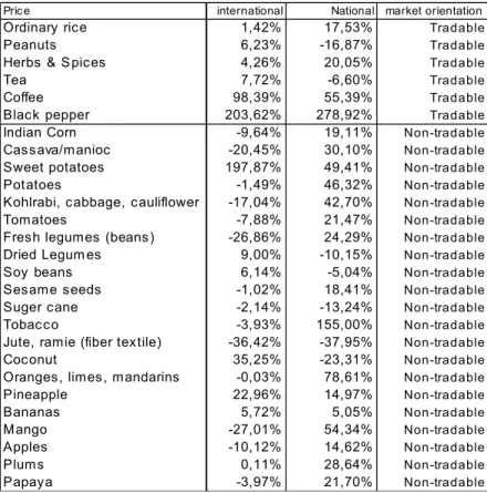
The major changes induced by trade liberalization impacted on agricultural prices and particularly the crops in which Vietnam had a comparative advantage. The impact was different across regions, as has been shown for rice market liberalization by Minot and Goletti (2000): they pointed out that the “Mekong River Delta produces rice surpluses. (...). Rice prices reflect these internal trade flows.” In line with the price analysis, as carried out by Edmonds and al (2004) for a spatial analysis of the rice price, I use provincial prices without regional deflators, in order to capture spatial prices variations induced by trade liberalization.
Price international National market orientation
Ordinary rice 1,42% 17,53% Tradable
Peanuts 6,23% -16,87% Tradable
Herbs & Spices 4,26% 20,05% Tradable
Tea 7,72% -6,60% Tradable
Coffee 98,39% 55,39% Tradable
Black pepper 203,62% 278,92% Tradable
Indian Corn -9,64% 19,11% Non-tradable
Cassava/manioc -20,45% 30,10% Non-tradable
Sweet potatoes 197,87% 49,41% Non-tradable
Potatoes -1,49% 46,32% Non-tradable
Kohlrabi, cabbage, cauliflower -17,04% 42,70% Non-tradable
Tomatoes -7,88% 21,47% Non-tradable
Fresh legumes (beans) -26,86% 24,29% Non-tradable
Dried Legum es 9,00% -10,15% Non-tradable
Soy beans 6,14% -5,04% Non-tradable
Sesame seeds -1,02% 18,41% Non-tradable
Suger cane -2,14% -13,24% Non-tradable
Tobacco -3,93% 155,00% Non-tradable
Jute, ramie (fiber textile) -36,42% -37,95% Non-tradable
Coconut 35,25% -23,31% Non-tradable
Oranges, limes, mandarins -0,03% 78,61% Non-tradable
Pineapple 22,96% 14,97% Non-tradable Bananas 5,72% 5,05% Non-tradable Mango -27,01% 54,34% Non-tradable Apples -10,12% 14,62% Non-tradable Plums 0,11% 28,64% Non-tradable Papaya -3,97% 21,70% Non-tradable
Table 1A : Evolution of national and international prices
National prices in Table 1A have been constructed from unit values at the household level. International prices are free on board (fob) world prices taken from the FAO.3 For comparability purpose, a deflator is imputed on January 1993 prices to obtain 1998 January prices.4
3See the variable description in appendix for more details on constructed variables. 4I uses as Benjamin and Brandt (2002) : 1.456.
Traded crops did indeed experience a huge price increase on average, compared to non-traded crops.5 On
average, national prices increase more than international prices.6 As labor costs were at first very low (on an
international basis) and fertilizer prices were nationally decreasing, Vietnamese prices were generally lower than international prices initially. The rise in national prices thus represented a convergence to the international level.
2.3
Inequality
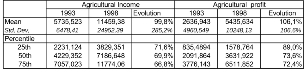
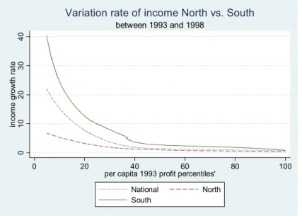
Table 1B shows the evolution of households’ agricultural profit and income between 1993 and 1998. Agricultural profit increases more than agricultural income, however the standard deviation shows a larger increase for agricul-tural income. Figure 1 gives the relative variation in agriculagricul-tural incomes, between 1993 and 1998, by initial per capita profit percentiles. The evolution was more favorable for the poorest households, especially in the South. Nevertheless, income distribution was still characterized by a high inequality. The Gini index for household agri-cultural income increased from 0.45 in 1993 to 0.53 1998. In the same way, the Theil coefficient jumped from 0.38 in 1993 to 0.62 in 1998. Inequality measures for profits describe a similar evolution to income, with a Gini index going from 0.47 in 1993 to 0.52 in 1998. 1993 1998 Evolution 1993 1998 Evolution Mean 5735,523 11459,38 99,8% 2636,943 5435,634 106,1% Std, Dev, 6478,41 24952,39 285,2% 4960,549 10248,13 106,6% Percentile 25th 2231,124 3829,351 71,6% 835,4894 1578,764 89,0% 50th 4229,352 7186,648 69,9% 2091,864 3631,922 73,6% 75th 7057,023 11774,06 66,8% 3776,143 6511,852 72,4%
Agricultural Income Agricultural profit
Table 1B: Agricultural profits and income evolution.
I split Vietnam in two agro-economic zones defined as the north and the south of the country.7 Figure 2 shows
that the distribution of land size was very unequal. These differences are exacerbated in the southern regions; where this unequal distribution of land is greater for the middle of the distribution. Figure 3 looks at the number of crops cultivated by a household, as a proxy for its degree of diversification (the opposite to its degree of specialization). If
5Traded crops represented in the top of Table 1A, have an average increase of 0.58 compared to 0.25 for non-tradable crops. Standard deviations are respectively 1.11 and 0.40. The non-tradable category without tobacco falls to a mean increase of 0.19 with a standard deviation of 0.28. Tradable crops without black pepper fall to a mean increase of 0.13, with a standard deviation of 0.28.
6Increases in international prices is about 53% for tradable crops and 5 % for non-tradable.
7A factor analysis has been done in order to find the major agro-economic zones.Whatthis shows is the existence of Northern and the Southern regions of Vietnam. The factors (the latent variable) were characterized by the 27 crops described in Table 1A and the observed variables used were the quantities (kg) produced by households.
0 10 20 30 40 in co me g ro w th r a te 0 20 40 60 80 100
per capita 1993 profit percentiles' National North South
between 1993 and 1998
Variation rate of income North vs. South
Figure 1: Income growth by region.
the analysis is broken down by regions, diversification is higher in the North, and the more so, for rich households, than in the South, where the number of crops is constant, whatever the agricultural income level of the household.8
These figures show a sharp contrast between the two major agro-economic regions and a strong inequality in both land and income distribution. However national unity in terms of tastes, culture and habits does exist, as pointed out by Figuie and Bricas (2003). Rice has always been the dominant staple, grown everywhere, even if the agro-economic zones have shown major differences, such as highland versus lowland and with different production techniques such as slash-and-burn and irrigation. In the panel sample rice is the main crop produced in both years.
3
Data
I use the two rounds (1992-1993 and 1997-1998) of the Vietnam Living Standards Survey (VLSS) in its panel dimension. As I am interested in the channels through which trade liberalization affected agriculture incomes, I limit my study to households that declared using some land. Thus the panel diminishes from 4300 households to 3076 households using land (representing 71 percent of the whole sample). The panel of agricultural households being sufficiently large, it was possible to create another panel based on the 27 crops cultivated in 1993 and 1998 with these 3076 households. Thus, the crop panel is composed of 8834 crop/households followed over the
8From know on, when I will talk about poor and rich households, this refers to the distribution of agricultural profit in 1993 (on which we compose percentiles).
50 00 10 00 0 15 00 0 20 00 0 25 00 0 19 93 la n d si ze 0 20 40 60 80 100
per capita 1993 profit percentiles' National North South
in 1993
Total household land size
Figure 2: 1993 levels of household total land size
2 4 6 8 10 12 19 93 nu m ber of c ro ps 0 20 40 60 80 100
per capita 1993 profit percentiles' National North South
in 1993
Number of crops evolution North vs. South
period 1993-1998. I also include all new varieties that households introduced or abandoned between both years, representing in total respectively 6519 and 4771 crops.
Households were distinguished according to the market orientation of their main crops, either traded or non-traded crops. This classification was created from COMTRADE data source for 1992, 1993, 1997 and 1998. I used the Vietnamese export values to define traded versus non-traded crops. Some of these crops did not appear at all in the COMTRADE list for any of these dates. For crops listed in the COMTRADE data set, I compose a total value exports for each of the 27th crops, averaged over every fourth years :92, 93, 97, 98. Two groups appear clearly: one with an average export value of $100 million, and another with an average export value of $5 million.9 In this classification, the export crops are the ones that are exported in large quantities, of which some have more or less been traditionally consumed by the Vietnamese. See Figuie and Bricas (2003) for a detailed analysis of Vietnam’s traditional food tastes.
4
Trade liberalization at a national level
This section computes the elasticity of local prices to international prices. The questions I want to answer are the following: are local prices sensitive to international prices during this period, the more so, if they correspond to traded crops or export-oriented crops ? Does the elasticity increase over time? Is the elasticity different depending on the agro-economic region ?
I start with a difference framework :
Pgrt= X e X t βetP∗ et.Iet+ X e X t λet.Iet (1)
where Pgrt is the price of crop g at year t in province r, P*et is the international price at year t=(93, 98) for e=(T, N) traded or non-traded crop, Ietis a dummy variable that indicates if the crop g is traded in year t or not. 10 Equation (1) is a summary form of a comparison between 1993 and 1998, for traded versus non-traded crops,
of the responsiveness of local prices to international prices.
Furthermore, as I want to understand how the elasticity of provincial prices to international prices can be explained by their distances to international markets, I introduce the distance between each province and the nearest commercial maritime port. Equation 1 becomes then :
9The median of the export crops listed on COMTRADE was 60M$ and the minimum value of the group equal to 33M$.The median of the non-export crops listed was 1M$ and the maximum value of 6M$.
Pgrt=
X
e
X
t
β1et(Pet∗ ∗ Distr).Iet+
X
e
X
t
β2et(Petr∗ ).Iet+
X
e
X
t
λet.Iet+ νr.Distr (2)
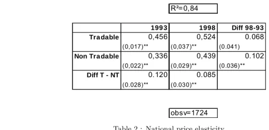
Table 2 shows how local prices respond to international prices. 84 percent of the variance of internal price is explained by international prices. According to the model, a one percent increase of the international price resulted in a 0.45 percent increase in the price of traded crops in 1993, holding all other variables constant. Traded price elasticity with respect to international price is higher than non-traded price. The elasticities increase over time, in a significant way, the more so for non-traded crops, as if the latter were catching up with traded crops.
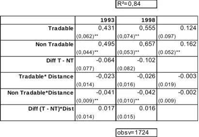
If the internal distances are introduced as control variables (table 3), the results are robust. The catch-up of non-traded crops is even more pronounced.
When differentiated by regions, as in tables 4 and 5, the difference estimation shows a strong difference between regions, as underlined by Benjamin and Brandt (2002). Most of the increase in price elasticity occur in the south region. In 1998, a one percent increase of international prices resulted in a 0.66 percent increase in south provincial prices of traded crops, holding all other variables constant. The south was more specialized in traded crops and land size per household was higher than in the north.
Last, tables 6 and 7 include the interaction of the variables with distance, as specified in equation (2). The price elasticity diminishes as the distance of the province to the port increases but only in the north provinces.11
To summarize, traded crops responded more to international prices than non-traded crops, both in 1993 and in 1998. The local price elasticity to international price increased over time especially in the south region. However, non-traded crops prices caught up more rapidly than traded crops with the international prices levels.
The provincial crop markets were connected to the international market. Distance mattered : the closer to a port the greater the elasticity to international prices.
R²=0,84
199 3 1998 Diff 98-93
Tra dable 0,456 0,524 0.068
(0,017)** (0,037)** (0.041)
Non Tra dable 0,336 0,439 0.102
(0,022)** (0,029)** (0.036)**
Diff T - NT 0.120 0.085
(0.028)** (0.030)**
obsv=1724 Table 2 : National price elasticity.
1 1In all tables, standard errors are in parentheses. Results are* significant at a 5% level of confidence; and ** significant at a 1% level of confidence.
R²=0,84
19 93 1998
Tra dable 0,431 0,555 0.124
(0,062)** (0,074)** (0.097)
Non Tra dable 0,495 0,657 0.162
(0,044)** (0,053)** (0.052)**
Diff T - NT -0.064 -0.102
(0.077) (0.082)
Trada ble * Dis ta nce -0,023 -0,026 -0.003
(0,014) (0,016) (0.019)
Non Tra dable*Dis ta nce -0,041 -0,042 -0.002
(0,009)** (0,010)** (0.009)
Diff (T - NT)*Dis t 0.017 0.016
(0.014) (0.015)
obsv=1724
Table 3 : National price elasticity interacted with distances.
R²=0,84
199 3 1998 Diff 98-93
Tra dable 0,435 0,419 -0.015
(0,023)** (0,040)** (0.046)
Non Tra dable 0,334 0,381 0.047
(0,025)** (0,041)** (0.045)
Diff T - NT 0.101 0.039
(0.034)** (0.036)
obsv=1075
Table 4 : North region price elasticity.
R²=0,86
199 3 1998 Diff 98-93
Tra dable 0,486 0,666 0.180
(0,025)** (0,059)** (0.065)**
Non Tra dable 0,355 0,528 0.173
(0,045)** (0,039)** (0.059)**
Diff T - NT 0.132 0.139
(0.052)* (0.048)**
obsv=649
Table 5 : South region price elasticity.
R²=0,84 1993 19 98 Tradable 0,404 0,52 0.115 (0,069)** (0,085)** (0.109) Non Tradable 0,606 0,723 0.117 (0,046)** (0,064)** (0.061) Diff T - NT -0.202 -0.203 (0.083)* (0.094)*
Tradable* Dis ta nce -0,043 -0,06 -0.017
(0,016)** (0,017)** (0.021)
Non Tradable *Dis ta nce -0,072 -0,071 0.001
(0,010)** (0,011)** (0.010)
Diff (T - NT)*Dis t 0.029 0.011
(0.016) (0.017)
obsv=1075
R²=0,86 1993 19 98 Tradable 0,558 0,622 0.064 (0,090)** (0,142)** (0.168) Non Tradable 0,24 0,544 0.304 (0,086)** (0,082)** (0.090)** Diff T - NT 0.318 0.078 (0.126)* (0.150)
Tradable* Dis ta nce -0,014 0,01 0.024
(0,02) (0,029) (0.032)
Non Tradable *Dis ta nce 0,022 -0,003 -0.026
(0,017) (0,015) (0.016)
Diff (T - NT)*Dis t -0.036 0.014
(0.022) (0.028)
obsv=649
Table 7 : South region price elasticity*distances
5
Effects of trade liberalization at the household level
I now turn to the impact of trade liberalization on agricultural incomes. The latter are defined as follows:12
Rh= X g qg(h)∗ pg(h)+ θh¡qg(h), pg(h) ¢ (3)
with Rh, real income of household h, qg(h), the quantity of crop g produced by the household h and pg(h),
household price (here, the unit value defined at a provincial level). Finally θh¡qg(h), pg(h)
¢
represent all other household incomes related to land, that will be a function of prices pg(h) and quantities qg(h).
If I write down the accounting equations for each year: 13
Rt= X g qgt∗ pgt Rt+1= X g qgt+1∗ pgt+1
1 2See variable description in appendix for details.
1 3For presentation purpose, we do not include the households subscript (h) _even if we are working at a household level_ and the others agricultural incomes _ but they are part of the agricultural income.
The variation of household income between (t) and (t+1) can be written as : Rt+1− Rt= X g [pgt+1− pgt] ∗ qgt+ X g [qgt+1− qgt] ∗ pgt+1 (4)
Equation (4) illustrates how agricultural households are affected by trade liberalization. The first term in the equation captures the price effect and the second term the quantity effect. However, the analysis is tricky because international prices affect not only local prices but also the quantities produced, through households’ decisions to re-allocate some land to a given crop. Alternatively, a household can also decide to stop cultivating a crop altogether; or, to start cultivating a new one. Moreover, the price and quantity of crop g can be influenced not only by international price P*g but also by the international price of another crop P*g’ (cross-substitution).
In order to simplify the framework, I introduce a reduced-form equation that will estimate a counter-factual income catching all effects due to the change in one international price. The idea is to classify households according to their ex-ante specialization which will alter their treatment (that is, their exposure to trade liberalization) as in Crepon and Deplatz (2001). A household would be more or less affected by the exogenous treatment (i.e. trade liberalization), according to his choice of specialization preceding this period. For this purpose, I construct a continuum of international price effects on 1993 quantities, and obtain an index that captures the degree with which household are affected by trade liberalization between 1993 and 1998. Thus it takes into account all effects related to prices and going either through the ”price channel” (first element of the RHS of equation (5)), holding crop choice constant.
I will first assess the share of observed agricultural household income variation that can be explained by this counter-factual ”international price-related” income. Secondly, I will explain agricultural household quantities variation through this continuous treatment methodology. Then I will look at agricultural household profits defined as households’ income minus households’ agricultural expenses. Finally all these variables will be studied through different specifications.
5.1
The reduced-form approach. Estimation of the direct effect of international
price.
Starting with the observed quantities in 1993 of crop g produced by household h, I calculate a fictive gain that isolates the price variation effect from changes in the specialization. This variable will be higher if, (1) a greater part of the land was dedicated by the household h to the crop g before trade liberalization and (2) the price of crop g after trade liberalization increased more than the other crops. I use two different prices. The first is an estimate of national prices and the second is based on provincial prices. Both prices are estimated as a function of international prices. The resulting estimated price variation is used to capture real income variation.
5.1.1 First Step: Definition of the price variation specification
As I have shown in section 4 that provincial prices were connected to international prices, I assume here that the difference in national prices depends the difference in international prices.
First specification with national estimated prices Pgt+1− Pgt= βg+ X g αg£p∗gt+1− p∗gt ¤ + εg (5)
I obtain a predicted difference in national prices : d Pgt+1− Pgt
Second specification with provinces estimated prices As in section 4, I use an alternative specification using provincial prices as dependent variables and distances to the nearest port :
Pgrt+1− Pgrt= βg+ X g αg £ p∗gt+1− p∗gt ¤ ∗ distr+ εgr (6)
Thus I obtain the estimation of the difference in local price for each of the sixty one provinces:
d Pgrt+1− Pgrt
5.1.2 Second Step: Construction of the income counterfactual
To measure the ex-post contribution of liberalization on agricultural household income, profits and quantities, it is necessary to control for some key households’ farm characteristics such as: total land size, number of cultures (specialization), share of the production sold in local markets, household’s land with a ”long term land use”. But it is essential to likewise control for specific households’ characteristics such as the education of household’s head, the number of individuals living in the household and the gender and age of the household head. Finally I will stratify the sample by regions (North and South), by quantiles of the agricultural profit distribution and quantiles of household total area distribution.
I follow the method used by Crepon and Desplatz (2001) that extends the method of matching normally used in discrete variable analysis. Here, the variations in agricultural household income is continuous in the sense that
they concern all households. Each of them will be affected differently according to the crop composition of their production. Thus I construct a households’ continuum of ex-ante effects for the two (national and provincial) specification of price variation.
First specification with estimated national prices. I use the predicted difference in prices obtained in (5) and compute a counterfactual income variation
g Rht+1− Rht = X g qght £ d pgt+1− pgt ¤ (7)
Second specification with estimated provincial prices. Alternatively, I use the provincial prices in equation (6) g Rht+1− Rht= X g qght £ d pgrt+1− pgrt ¤ (8)
5.1.3 Third Step: Estimation of the gap between observed and counterfactual income variation.
The reduced form equation allows to measure the effect of the ”treatment” (here, trade liberalization) on households’ incomes. It writes :
Yt+1− Yt= ζh+ γRht+1g− Rht+ ωh (9)
The counterfactual income variationRht+1g− Rhtgives the exposure of agricultural households to trade
liberal-ization occurring through the price pass-through. This counterfactual income variation is compared to the observed variation in outcome Yt+1− Yt. Accordingly the coefficient of interest is then γ. The R2 indicates which part of the
evolution of the dependent variable dispersion is simply explained by the initial specialization and the variation in international prices.
If Yt+1− Yt is the observed change in agricultural income, a coefficient γ equal to one would indicate that
households have stayed with their initial specialization.14 It is thus interesting to disaggregate the effect on a
stratified sample: at a geographic level, along the profit distribution and along the land area distribution.
I am also interested by analyzing the impact of the liberalization process on different outcomes other than income. Two alternative specifications of equation 9 will be explored, where the dependent variable will be first the quantities produced, and second, agricultural profits. This is justified by the fact that a household, given its ex-ante specialization and prices’ evolutions, has the possibility to maximize its gains by extending the area of the produced crop and/or by adopting inputs in order to increase its productivity. Profits, on the other hand, are interesting to look at, as they include all expenses related to farm activities which could be greatly differentiated accross population groups.15 Studies on Vietnam agricultural productivity have shown up that a major factor the
increase in inputs use (more particularly fertilizer). The specification with the profit outcome allows to understand what has been the net gain of trade liberalization for agricultural households.
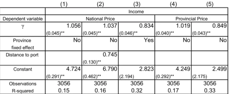
(1) (2) (3) (4) (5) Dependent variable γ 1.056 1.037 0.834 1.019 0.849 (0.045)** (0.045)** (0.046)** (0.040)** (0.043)** Province No No Yes No No fixed effect Distance to port 0.745 (0.130)** Constant 4.724 6.790 2.823 4.249 2.499 (0.291)** (0.462)** (2.194) (0.292)** (2.175) Observations 3056 3056 3056 3056 3056 R-squared 0.15 0.16 0.32 0.17 0.33 Income
National Price Provincial Price
Table 8 : Estimation of agricultural income.
The coefficient γ in Table 8 is not statistically different from one if provinces’ controls are not included. Accord-ingly a one dong increase in the outcome of the counter-factual ”international price-related” income will induce a one dong increase in variation of agricultural income, ceteris paribus. Provincial prices (column 3) have a higher R2 than national prices (column 1), thus provincial prices predict better the real income variation of households than the national prices, ceteris paribus.16 Another interesting, perhaps surprising result, comes from the positive
coefficient of the distance to a port. The farther the household is from the port, the higher is the increase in his income. This possibly comes from the catching up of provinces that were isolated from the national market and, a fortiori, from the international markets. This catching up is in line with the fact that non-tradable prices experienced the largest increase in terms of elasticity with resspect to international prices (see above, Section 4).
1 4Another more unlikely explanation could be that there were some changes in specialization but they cancelled each other ( a change in specialization toward a crop that ended negatively affected by trade liberalization was completely compensated by a change in specialization toward a crop positively affected by trade liberalization. )
1 5For expenses details see appendix.
(1) (2) (3)
Dependent variable National North region South region
γ 0.750 0.229 0.946
(0.045)** (0.032)** (0.087)** Num ber of crop -0.466 0.030 -0.411
produced (0.060)** (0.033) (0.279) Long term use 0.375 0.069 0.085
(0.074)** (0.058) (0.147) % of sales 4.879 -0.517 3.074
on local market (1.001)** (0.697) (2.008) Household total area 1.796 1.064 1.906
(0.290)** (0.215)** (0.544)**
Age 0.041 -0.078 0.159
(0.112) (0.067) (0.258)
Age² -0.001 0.000 -0.002
(0.001) (0.001) (0.003) Prim ary education 0.687 -0.026 2.441
(0.662) (0.397) (1.440) 2nry education -0.620 0.578 0.764
& beyond (0.714) (0.402) (1.958) Technical education -1.167 0.214 -1.311
(0.999) (0.501) (3.727) Num ber of individuals 0.540 -0.009 0.857
in the household (0.130)** (0.084) (0.270)** Head is a -1.344 -0.637 -1.443 wom an (0.627)* (0.338) (1.537) Head is tay 2.351 1.443 7.333 (1.414) (0.625)* (8.729) Head is thai -2.073 -0.400 0.085 (2.114) (1.034) (6.538) Head is chinese -2.585 -0.713 -3.101 (3.959) (5.504) (6.257) Head is khmer -0.303 -2.910 -1.548 (1.751) (3.886) (2.692) Head is Muong -3.487 -2.039 (1.512)* (0.662)** Head is Nung 2.974 2.171 (1.663) (0.719)** Head is Hmong (meo) -5.660 -1.108
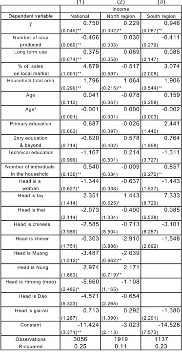
(2.482)* (1.165) Head is Dao -4.571 -0.654 (5.323) (2.265) Head is gia-rai 0.713 0.292 -1.380 (1.287) (1.090) (2.291) Constant -11.424 -3.023 -14.528 (3.371)** (2.113) (7.573) Observations 3056 1919 1137 R-squared 0.25 0.11 0.23 Income
Table 9 : Regional estimation of agricultural income.
In Table 9, in order to capture variables that could have had a causal effect on household income variation, I control for other factors. The coefficient γ is not different from one in the southern region. For the northern region the coefficient γ is less than 1. It might be the case that an omitted variable diminishes the direct impact of international price on income. It could be for example that households located in the north have not managed
to adjust their culture toward crops whose prices evolved favourably.17
In particular, the evolution of incomes is negatively correlated with the fact that the household head is a woman. The lower the number of crops a household produces (the lower the diversification) the higher the increase in income between 1993 and 1998. Agricultural income variation is also posively associated with the number of individuals living in the household. However these last two result do not hold in the northern region. Moreover the growth of agricultural income in negatively correlated with the fact that the household head is Muong relatively has being Kinh.
Farm variables indicate that a larger total land size and a larger share of household production sold are positively correlated with income evolution. Finally area on a "long term land use” is correlated with a higher increase in income.
(1) (2) (3)
Dependent variable National North region South region
γ 0.099 0.004 0.127
(0.014)** (0.017) (0.024)** Control hsld Yes Yes Yes
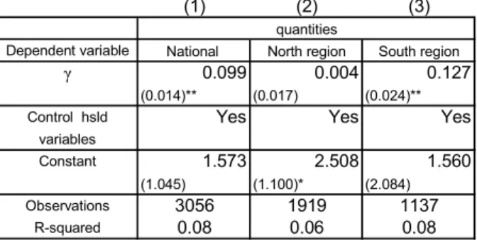
variables Constant 1.573 2.508 1.560 (1.045) (1.100)* (2.084) Observations 3056 1919 1137 R-squared 0.08 0.06 0.08 quantities
Table 10 : Regional estimation of quantities.
I look now at the quantities variation of agricultural households. Table 10 shows that, for the southern region, the more households have been affected by trade liberalization, due to their ex-ante specialization, the greater the increase in quantities produced. Conversely, in the North, no difference is found on the volume of output produced between households affected by trade liberalization or not.18 I turn now to the stratified impact of trade
liberalization in terms of agricultural profits, on agricultural income and land distribution.19
1 7We will answer to this hypothesis later.
1 8From now on, results on control variables are not shown for a clarity purpose. They can be provided by the author on request. 1 9”Low” profit earners or ”poor” are the households for which total agricultural profit is equal or inferior to the 25th percentile of the 1998 distribution. ”High” profit earners or ”rich” are those for which profit is equal or superior to the 75th percentile of the 1998 distribution. I choose to look at 1998 profit distribution because we are interested to understand through which channel vietnamese households have became winners or losers of this period of trade liberalization.
(1) (2) (3) (4) (5) (6) (7) (8) (9)
National North South National North South National North South γ * median 0.074 0.020 0.215 -0.118 -0.051 -0.219 -0.093 -0.007 -0.220 (0.084) (0.041) (0.212) (0.027)** (0.024)* (0.059)** (0.056) (0.032) (0.139) γ * low 0.579 -0.031 1.049 0.043 -0.064 0.111 -0.369 -0.099 -0.515 (0.072)** (0.042) (0.148)** (0.023) (0.025)* (0.041)** (0.048)** (0.033)** (0.097)** γ * high 0.961 0.885 0.862 0.173 0.166 0.146 0.529 0.359 0.444 (0.055)** (0.051)** (0.094)** (0.017)** (0.030)** (0.026)** (0.036)** (0.040)** (0.062)** low -3.098 -2.486 -2.756 -0.959 -0.649 -1.282 -3.033 -2.704 -4.250 (0.639)** (0.306)** (1.758) (0.201)** (0.180)** (0.487)** (0.424)** (0.236)** (1.153)** high 7.083 2.680 12.705 1.695 1.283 1.953 5.800 3.359 8.549 (0.688)** (0.376)** (1.679)** (0.216)** (0.221)** (0.465)** (0.456)** (0.290)** (1.101)**
Control variables Yes Yes Yes Yes Yes Yes Yes Yes Yes
Constant -4.795 4.896 -10.763 3.425 4.923 2.706 -3.252 5.730 -11.543
(3.152) (1.822)** (7.104) (0.993)** (1.072)** (1.971) (2.090) (1.405)** (4.658)* Observations 3056 1919 1137 3056 1919 1137 3056 1919 1137
R-squared 0.36 0.38 0.33 0.19 0.16 0.20 0.37 0.35 0.37
income quantities Profits
Table 12 : Change in regional income, profits and quantities by profits quantile.
Table 12 shows (column 1) that rich households experienced a positive income variation while poor households were.negatively affected If taking into account for ex-ante specialization the results are less contrasted, the low profit earners benefited from trade liberalization in the same order of magnitude as large profit earners (coefficients are not statically different at a 1% level of significance) The phenomenon is more accurate in the South (column 3) where the impact of trade liberalization has been more uniform on low and high profit earners.20 On the other hand,
in the North (column 2) high profit earners benefitted most from liberalization and interaction of counterfactual income variation and small profits is not significant. Concerning quantities (columns 4-6) counterfactual income variation in the South for the poor has a positive effect, which is not verified in the North. Rich households with a favourable ex-ante specialization have increased their quantities in the same terms as poor households affected by trade (coefficient are not statistically different).
Finally, columns 7-9 take as dependent variable the agricultural profits. Expected results are lower than income evolution results as expenses are subtracted. Poor households with favourable initial specialization who earned more in terms of income, had a negative evolution of their agricultural profits. This result is particularly surprising for the South region, where this negative effect is even more pronounced than in the North.
(1) (2) (3) (4) (5) (6)
National North South National North South γ * other 0.201 0.024 0.560 0.048 -0.028 0.134 (0.093)* (0.046) (0.265)* (0.067) (0.036) (0.193) γ * small plot 0.632 -0.027 0.841 -0.713 -0.074 -1.187 (0.258)* (0.193) (0.487) (0.187)** (0.151) (0.355)** γ * large plot 0.883 0.423 0.930 0.273 0.143 0.246 (0.051)** (0.044)** (0.089)** (0.037)** (0.034)** (0.065)** small plot of land -1.611 -1.612 -0.061 0.153 -0.986 1.589
(0.757)* (0.424)** (1.916) (0.551) (0.332)** (1.400) large plot of land 2.211 -0.568 5.970 1.592 -0.455 3.016
(0.802)** (0.499) (1.851)** (0.583)** (0.391) (1.354)*
Control variables Yes Yes Yes Yes Yes Yes
Constant 4.851 6.896 2.674 -1.097 3.074 -8.941
(2.587) (1.447)** (6.348) (1.883) (1.135)** (4.644) Observations 3056 1919 1137 3056 1919 1137
R-squared 0.26 0.13 0.24 0.13 0.06 0.10
income profit
Table 13 : Change in regional income by land quantiles.
Table 13 shown the results when households are categorized as users of large and small plots of land .21 Column 1 shows a positive effect of large land users and negative effect on income for small users. Nevertheless if initial crop specialization was favorable, using a small plot has a positive impact on income variation. This effect is however not robust for small plot when looking at regional level (column 2 and 3). One the other hand even with an ex-ante specialization in crops favoured by trade liberalization, small plot users saw a decrease in their profits due to trade liberalization while large profit earners benefitted. At a regional level, households in the South had on average a higher land size Finally estimations on quantities indicate that users of small and medium land plots have not been able to take advantage, of their initial specialization. 22
To sum up, this exercise consisting in measuring the effect of trade liberalization on agricultural households has shown very sharp contrast between segments of the population. The reduced form has allowed to evaluate the evolution of various variables of interest such as income, profits and quantities. We have seen that Southern Vietnam has been positively affected by trade liberalization relatively to the Northern region. This differentiation between the agro-economic regions could be explained by the fact that in the South households were able to re-allocate its production in terms of quantities when affected by trade liberalization. Then one of the first conclusions at regional level is that households in the Northern region affected by trade liberalization have not had the chance to re-allocate their production choices during this period of openness to international markets.
First at a national level, trade liberalization had a positive effect on agricultural income of poor and rich households. Second, poor households in the South, with an initially good specialization , have been able to
2 1Households considered as users of small land plots if the area cultivated is equal or inferior to the 25th percentile of the total area distribution. Large land plot are those equal or superior to the 75th percentile of the total area distribution.
adjust their quantities in order to take advantage of price evolution. It resulted that poor Vietnamese agricultural households in the southern region with an ax-ante favorable crops specialization have had strong positive evolution of their agricultural income.Agricultural profits did not gain from trade liberalization. This is due
favourable evolution of their quantities compared to poor households in the Northern region. Therefore it can be said that the extension of quantities initiated by poor households giving their ex-ante specialization in the South has been a success.
But at this stage of the process of trade liberalization expenses are still higher than incomes and thus invest-ments in inputs have been very costly leading to negative profits for poor and positive for rich households even when possessing favourable initial specialization. The overall consequence is that controlling for the ex-ante crop specialization in the end, southern poor households lose more than poor in the northern region.
6
Conclusion
We have shown an original ex-post analysis of the effects of trade liberalization in rural Vietnam between 1993 and 1998, taking into account the regional differentiation of the Vietnamese economy. The impact of trade liberalization is firstly analyzed through the changes induced in domestic prices, and then on household income with a continuous treatment methodology as Crepon and Deplatz (2001).
The results suggest that trade liberalization has affected domestic prices and agricultural income differently both through production specialization and geographical distribution. Therefore trade liberalization produced differentiated outcomes according to the degree by which households have been affected by this liberalization. Regarding prices, the results show that tradable crops are highly sensitive to international prices, and particularly the southern region of Vietnam. Due to the large share of exporters present in the south that have been more positively affected by trade liberalization, the agricultural income gap between the north and the south has widened further. Moreover effects of trade liberalization on local price have been lowered by the distance to the commercial port for non tradable crops.
Findings on agricultural income confirm the hypothesis that trade liberalization has been more pro-rich in the northern region, while in the south it has had more uniform effects both for rich and poor households. This phenomenon seems to be due to the possibility for poor households to strongly increase their quantities and thus to take advantage of the price increases. However if expenses are deducted then the situation reverses and poor’s profits became negative in the southern region, resulting in a mitigated situation. The segmentation of the agricultural population through their cultivated area shows great inequality during this period of trade liberalization. Indeed agricultural income has uniformly increased for users of small and large land plots whereas at the same time users of large plots have seen a huge increase in their profits. Finally the users of small plots have seen a large decrease of their profits especially for households in the South.
In conclusion, at this stage of trade liberalization, agricultural markets have witnessed an increased inequality within the country, with a negative evolution of profits for the poorest.
References
[1] Athukorala (2005) ‘Trade Policy Reforms and the Structure of Protection in Vietnam’ Research School of Pacific and Asian Studies, Australian National University.
[2] Auffret P. (2003). Trade Reform in Vietnam Opportunities with Emerging Challenges. World Bank Policy Research Working Paper No. 3076.
[3] Benjamin D. & Brandt L.. (2002). Agriculture and Income Distribution in Rural Vietnam under Economic Reforms: A Tale of Two Regions. William Davidson Institute Working Papers Series 519.
[4] Crépon B., Desplatz R. (2002).Une nouvelle évaluation des effets des allégements de charges sociales sur les bas salaires. Economie et statistique,n◦348, 2001-8
[5] Edmonds E. and Pavcnik, N.(2004). Product Market Integration and Household Labor Supply in a Poor Economy: Evidence from Vietnam, World Bank Policy Research Working Paper #3234.
[6] Figuie. M et Bricas N. (2003) Evolution de la consommation alimentaire au Vietnam. (Eds.). Marché alimen-taire et développement agricole au Vietnam. Hanoi, Malica (CIRAD-IOS-RIFAV-VASI). pp. 36-47.
[7] Gallup J. L. (2003). The Wage Labor Market and Inequality in Vietnam in the 1990s World Bank Policy Research Working Paper No. 2896.
[8] Lavigne M. (1999) Economie du Vietnam_ Réforme, ouverture et développement, Collection “Pays de l’Est », L’Harmattan.
[9] Litchfield & Justino (2002). Welfare in Vietnam during the 1990’s : Poverty, Inequality and poverty dynamics. Journal of the Asia Pacific Economy, volume 9 (2), p.145-169.
[10] Paquet E. (2004) Réforme et transformation du système économique Vietnamien 1979-2002, Collection “Pays de l’Est », L’Harmattan.
[11] Minot, N. and F. Goletti (2000). Rice Market Liberalization and Poverty in Viet Nam IFPRI Research Report No 114. Washington, D.C.
7
Appendix A: Variables description
The crop provincial price(Prg) is created through the households’ unit values. The variable used to compose
these unit values is the ratio of quantities on values sell on the local market. Then average unit values are created by crop and provinces, I drop the highest and lowest one percent values. Each value reported by the household to composed the unit value, as been deflated by a month deflator. The unit is in thousands Dongs per kilograms.
The crop national price³Pgt= P61
r=1Pgrt∗ngrt Ngt
´
is create through the crop provincial price Pgrt. The variable is weighted by the number of household by provinces³P61r=1ngtr = Ngt
´ .
The household agricultural income (Rh(r)) has been composed via agriculture section of the VLSS. The
household output of each crop is the quantity harvested (in kilograms) per the provincial unit value (as explain in the upper paragraph): ”crop provincial price”).23 Plus incomes provided from land use.
The household agricultural profits include the household agricultural income. From which has been subtracted all expenses related to agricultural activity including : the purchase of inputs (seeds, fertilizer...), the payment of external farm employment, and the expenses related transportation, storage, agricultural taxes, etc. . .
The international prices (P∗
gt ) have been created from Faostat data. For each of the crops I have divided
the “Export Value” variable by the “Export Quantity” variable for the “World”. For comparison purpose, the international prices given in thousand dollars per millions of tons are transformed in thousand Dong per kilograms (exchange rates have been founded on ”http://www.unhchr.ch/tbs/doc.nsf/(Symbol)/E.C.12.1993.SR.9.Fr” and ”http://projetscours.fsa.ulaval.ca/gie-64375/vietnam/site/crise.htm” for 1993 and 1998 respectively)
The distance to the nearest port (dr ) have been created by the author, it’s an average distance of the
province’s capital to the nearest port (Dong Hoi, Haiphong Ho Chi Minh and Quy Nhon ). The value of one has been attributed to provinces that include these ports.
Household Mkt: ³= P gQte_ Sold P gQte_total ´
It’s a variable at the household level that resumes the share of household’s production that is sold on markets. It’s defines as the ratio of the sum of quantities sold on the market on total quantities produced.
Region
-North include: Red River Delta, North East, North West, North Central Coast.
-South include: South Central Coast, Central Highlands, North East South, Mekong River Delta.
2 3Including crop listed on table 1A and all other crops for which it was not possible to find an international price and all categories labelled as ”others...”.