Process-oriented statistical-dynamical evaluation of LM precipitation forecasts

(1)

HAL Id: hal-00297084

https://hal.archives-ouvertes.fr/hal-00297084

Submitted on 9 Apr 2008

HAL is a multi-disciplinary open access

archive for the deposit and dissemination of

sci-entific research documents, whether they are

pub-lished or not. The documents may come from

teaching and research institutions in France or

abroad, or from public or private research centers.

L’archive ouverte pluridisciplinaire HAL, est

destinée au dépôt et à la diffusion de documents

scientifiques de niveau recherche, publiés ou non,

émanant des établissements d’enseignement et de

recherche français ou étrangers, des laboratoires

publics ou privés.

Process-oriented statistical-dynamical evaluation of LM

precipitation forecasts

A. Claußnitzer, I. Langer, P. Névir, E. Reimer, U. Cubasch

To cite this version:

A. Claußnitzer, I. Langer, P. Névir, E. Reimer, U. Cubasch. Process-oriented statistical-dynamical

evaluation of LM precipitation forecasts. Advances in Geosciences, European Geosciences Union, 2008,

16, pp.33-41. �hal-00297084�

(2)

www.adv-geosci.net/16/33/2008/

Geosciences

Process-oriented statistical-dynamical evaluation of LM

precipitation forecasts

A. Claußnitzer, I. Langer, P. N´evir, E. Reimer, and U. Cubasch

Institut f¨ur Meteorologie, Freie Universit¨at Berlin Carl-Heinrich-Becker-Weg 6-10, D-12165 Berlin, Germany Received: 1 August 2007 – Revised: 10 January 2008 – Accepted: 29 February 2008 – Published: 9 April 2008

Abstract. The objective of this study is the scale dependent

evaluation of precipitation forecasts of the Lokal-Modell (LM) from the German Weather Service in relation to dy-namical and cloud parameters. For this purpose the newly de-signed Dynamic State Index (DSI ) is correlated with clouds and precipitation. The DSI quantitatively describes the devi-ation and relative distance from a stdevi-ationary and adiabatic so-lution of the primitive equations. A case study and statistical analysis of clouds and precipitation demonstrates the avail-ability of the DSI as a dynamical threshold parameter. This confirms the importance of imbalances of the atmospheric flow field, which dynamically induce the generation of rain-fall.

1 Introduction

In the last years the development of numerical weather pre-diction (NWP) models there has been great progress in the short-term and middle-term forecast of temperature, wind speed or direction and cloud coverage, but only minor suc-cess in the quantitative precipitation forecast (QPF). In order to improve the NWP models, it is necessary to understand the precipitation processes. In general, rainfall is a very dis-continuous variable in space and time. It is difficult to obtain spatial-temporal information about precipitation on the ob-servational as well as on the modelled basis.

Physically, in the mid-latitudes rainfall develops via the ice phase in the clouds, the so-called Bergeron-Findeisen-Process. In synoptic meteorology, precipitation is linked to upward vertical motion in large-scale baroclinic systems. In particular, in the mid-latitudes high correlations of precip-itation rates and vertical velocity can be found (Rose and

Correspondence to: A. Claußnitzer (antje.claussnitzer@met.fu-berlin.de)

Lin, 2003). Alternatively, the ageostrophic horizontal diver-gence weighted with the specific humidity is used to esti-mate diagnostic precipitation rates (Spar, 1953; Palm´en and Holopainen, 1962; Banacos and Schultz, 2005). Other re-search groups deal with the statistical analysis of precipita-tion processes to investigate a multifractal (e.g. Olsson et al. , 1993; Tessier et al., 1993; Lovejoy and Schertzer, 1995) and a chaotic behaviour (Rodriguez-Iturbe et al., 1989; Sivaku-mar, 2001). In particular, there is an indication that convec-tive precipitation is linked to self-organised critical phenom-ena, with the saturation of water vapour as the dynamical threshold (Peters and Christensen, 2006). A previous study from Langer and Reimer (2007) shows an improvement by considering the clouds types derived from Meteosat-7 for an independent numerical interpolation procedure to build up an observational precipitation analysis in a resolution corre-sponding to the LM grid (Reimer and Scherer, 1992).

The aim of this paper is to present a connection between the Dynamic State Index (DSI ), which skillfully combines the above-mentioned imbalances of the flow fields, and pre-cipitation as well as clouds. The paper is divided into the following parts: Sect. 2 gives a short description of the DSI and Sect. 3 specifies the Meteosat-8 channels and the derived cloud types. The data sets used as well as the calculation of the DSI and cloud types are presented in Sect. 4. The results of this study are given in Sect. 5, organised in three themes. First the correlation between the DSI and the precipitation derived from the LM data is presented, then a case study shows the exceeding agreement in space. In the last subsec-tion Meteosat-8 data are used and with a new approach the precipitation activity of different cloud types is calculated. Finally Sect. 6 gives a summary.

(3)

34 A. Claußnitzer et al.: Process-oriented statistical-dynamical evaluation of LM precipitation forecasts

S

S N

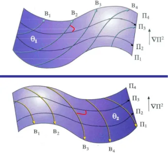
Fig. 1. Isolines of 5 and Bernoulli-stream function on two different

isentropic levels θ1and θ2. The red lines indicate angles between

Bernoulli streamfunctions and PV isolines with 54> 51.

2 Dynamic State Index DSI

Usually, precipitation is a parameter, which is linked to changes in the atmospheric circulation, e.g. growth of baro-clinic waves and frontogenesis on the synoptic scale. It is also coupled with the mesoscale convective system (e.g. Houze, 2004). These meteorological phenomena can be at-tributed to non-balanced processes. The newly designed Dynamic State Index (DSI ) describes the deviation from the stationary solution of the adiabatic primitive equations (N´evir, 2004) and is in this way a measure of non-balanced properties of atmospheric flow fields. The above-mentioned solution describes a generalised geostrophic equilibrium, which can be expressed in terms of a three-dimensional sta-tionary velocity vector vst:

vst=

1

ρ5∇θ × ∇B· (1)

Here θ denotes the potential temperature, 5 is Ertel’s poten-tial vorticity (PV), B the Bernoulli-stream function and ρ the density of air. For a classical derivation in terms of the gov-erning equations see Sch¨ar (1993). The DSI is defined as a Jacobian determinant:

DSI := 1 ρ

∂(θ, 5, B)

∂(x, y, z) , (2)

which locally includes the information about entropy, en-ergy and potential vorticity and describes diabatic and non-stationary processes of the atmospheric flow field. Because

of the functional dependence of the Bernoulli-stream func-tion and the PV in the stafunc-tionary energy-vorticity basic state the index in this state is exactly zero (DSI =0). The oscil-lation around the basic state is visualised by spatial dipole structures in the horizontal plane. In this way the DSI is used as a dynamical threshold parameter for precipitation processes. An application of the DSI with respect to the visualisation of storm tracks and the evolution of severe win-ter storms and hurricanes can be found in Weber and N´evir (2008).

2.1 Physical and geometrical interpretation of the DSI In this section it will be shown that the DSI in the non-balanced state is proportional to the advection of the squared

5. Rewriting the definition of the DSI (Eq. 2) as scalar

triple product [a · (b × c)] and using the stationary velocity

vst(Eq. 1), the DSI can be rewritten in the following way:

DSI = 1 ρ∇5(ρ5vst) = vst· ∇ 52 2 ! . (3)

Under general conditions the atmospheric flow is certainly not in the energy-vorticity equilibrium, so the stationary wind becomes the real, non-balanced wind. Therefore two cases have to be distinguished:

DSI =                vst· ∇ 52 2 ! =0 v · ∇ 5 2 2 ! 6=0 . (4)

In addition to the mathematical derivation a geometrical interpretation together with a discussion of the sign of the

DSI is given in Fig. 1. Here the isolines of the Bernoulli

stream function and the PV are shown on two isentropic surfaces. In the case of vanishing DSI the isolines of the Bernoulli stream function and the PV are parallel. On the θ1

-surface, an angle between 0–90◦denotes a DSI >0. Accord-ing to Eq. 4 this implies a negative advection of the squared PV. On the θ2-surface, an angle between 90–180◦denotes a

DSI <0, which implies a positive advection of the squared

PV.

3 Cloud types derived from satellite data

The products “cloud classes” and “cloud coverage” derived from Meteosat-8 data are uses with a temporal resolution of 15 min. The original resolution of the Meteosat infrared data is 3×3 km2. Meteosat-8 data are transformed into a geographic projection with an effective spatial resolution of 0.01◦. For the correction of the sun’s elevation, the cosine of the zenith distance was used. In order to determine the

(4)

cloud classes and the cloud cover, the near-infrared channels at 0.6 and 0.8 µm, called VIS06 and VIS08, and the ther-mal infrared channel at 10 µm (VIS10) from Meteosat-8 be-tween 06:00UTC and 18:00UTC were selected. The cloud classification from satellite data is based on the distribution of clouds in different heights (i.e. with different cloud top temperatures) and with different optical thicknesses in a bi-spectral histogram (Berger, 1992; Langer and Reimer, 2007). One extreme case is the cloudless surface which should be the warmest and darkest area in the satellite image and the other extreme case is the cloud top of a cumulonimbus as the coldest and brightest area. The automated classification scheme tries to find those areas and builds test classes for other cloud types and calculates the arithmetic mean and the covariance for each class (Berger, 1992). For each pixel in the satellite image the probability of membership in the different classes is tested and the pixel is assigned to the class having the highest probability (Maximum-Likelihood-method). From Meteosat-8 data four cloud types in the high level are determined: cirrus spissatus, cirrus fibratus, cirrus spissatus cumulonimbogenitus and cirrostratus, grouped to-gether in the cirrus class. The medium-high clouds are de-termined by two cloud types, altocumulus translucidus and altocumulus together with altostratus/nimbostratus. The low clouds are separated into six cloud classes: cumulus hu-milis, cumulus mediocris, cumulus/stratocumulus, cumulus congestus, stratus fractus (higher clouds not visible from the ground), cumulonimbus or nimbostratus. In fact, cumu-lonimbus and nimbostratus do not occur at the same time. If the nimbostratus has a cirrus layer above it, the radiation characteristics due to the satellite channels are very simi-lar to those of cumulonimbus and a separation of the cloud type is only possible with the help of the weather type from synoptic-based stations (Xie and Arkin, 1995).

4 Data sets

4.1 Precipitation data

The Lokal-Modell (LM) of the German Weather Service (DWD) is a non-hydrostatic limited-area atmospheric pre-diction model with 325×325 grid points and a horizontal grid resolution of 0.0625◦ (≈7 km) (Doms and Sch¨attler, 1999). Data from 2000 to 2004 were used for the evalua-tion of the LM hourly precipitaevalua-tion. Besides that, one year of LM-analysis and forecast data, from March 2004 to Febru-ary 2005, was analysed. The LM-forecast data are based on 00:00 UTC runs and have the same spatial and tempo-ral resolution as the analysis data. The LM precipitation forecast data are cumulative, from the start of the forecast run. To obtain the hourly rainfall information of this time period, the successor minus the predecessor was calculated. The following one-level-fields rainfall can be retrieved from the DWD data base: grid-scale rainfall, convective rainfall,

grid-scale snowfall, convective snowfall and the total precip-itation. The cumulus parametrization scheme according to Tiedtke (1989) uses a mass-flux approach to represent moist convection in the LM. In the LM cumulus convection is a sub scaled process in the LM, which is not resolved from the grid and can therefore not be simulated explicitly. To obtain the whole grid scale (stratiform) and convective pre-cipitation, the parts of rain and snow were added to the total stratiform precipitation (TG) and the total convective precip-itation (TC). The total precipprecip-itation (TP) is the sum of total convective and total stratiform precipitation.

4.2 Input data for DSI calculation

The DSI is evaluated on nine isentropic levels over the whole LM-domain (325×325 grid points), for a time period of five years (2000–2004). For this purpose, successive Jan-uaries and Julies were selected to analyse characteristic sea-sonal precipitation patterns. The DSI is also assessed for one year, ranging from March 2004 to February 2005, with LM-analysis and forecast data in the same time frame as the precipitation data. The input data (zonal wind u [m/s], merid-ional wind v [m/s], temperature T [K] and geopotential 8 [m2/s2]) are available from LM-analysis and forecast fields with a time resolution of one hour. The LM variables are in-terpolated on ten pressure levels (Doms and Sch¨attler, 1999). The isentropic analysis scheme of Reimer and Scherer (1992) has been used to interpolate the LM-data from pressure lev-els to θ -surfaces. The resulting isentropic levlev-els are 260 K, 280 K, 300 K, 320 K, 330 K, 340 K, 350 K, 360 K and 390 K. The determinant (Eq. 2) is calculated in isentropic coordinates and PV, Bernoulli-function, gradients in x- and

y-direction were derived on θ -levels. The DSI -fields are

compared with LM precipitation (TP, TG, TC). 4.3 Cloud data

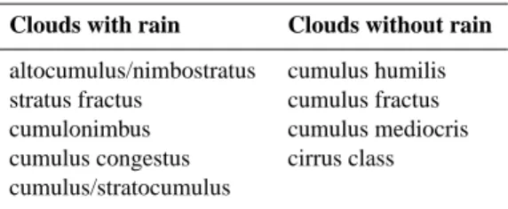
For the comparison between DSI and the cloud types the period February to December 2004 was analysed. The con-sidered domain covers “Central Europe” from 5.0◦E/39.6◦N to 20.4◦E/39.6◦N and 20.4◦E/55.0◦N to 5.0◦E/55.0◦N. The cloud data have the same spatial and temporal resolution as the calculated DSI -data, corresponding to a smaller grid of 201×249 grid points. The cloud classification derived from Meteosat-8 data for the eleven month of the year 2004 of-fers the possibility to attribute a precipitation probability to special cloud types. Therefore “rain clouds” and “no rain clouds” can be distinguished. Clouds with rain are: altocu-mulus/nimbostratus, stratus fractus, cumulonimbus, cumu-lus/stratocumulus and cumulus congestus and clouds with-out rain are cumulus humilis, altocumulus and cumulus mediocris and the cirrus class. Only the data sets of the

DSI and cloud types from Meteosat-8 between 09:00 and

16:00 UTC are used, due to the sunshine duration (Langer et al., 2008).

(5)

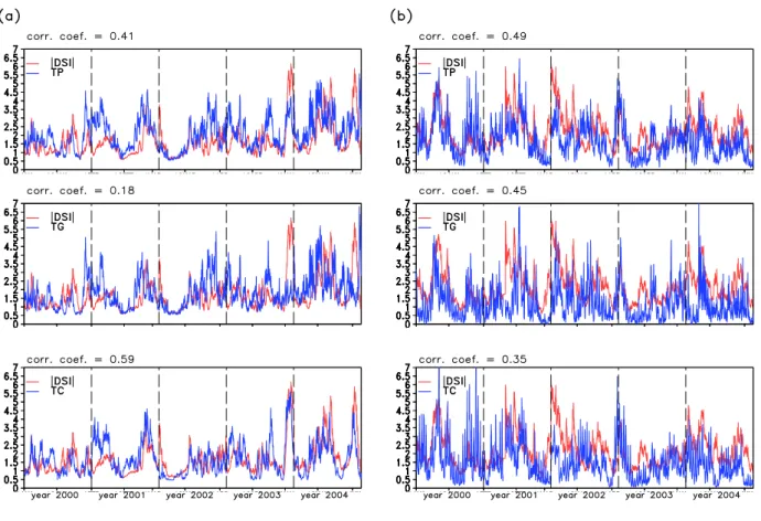
Fig. 2. Correlation coefficient between area means of |DSI | and precipitation (total precipitation (TP), total stratiform (TG) and total

convective precipitation (TC)) for successive Januaries (a) and Julies (b), based on hourly LM-analysis data (2000–2004, whole LM-domain of 325 x 325 grid points, scaled by standard deviation). The considered isentropic level is 320 K.

5 Results

5.1 Correlation between LM precipitation analysis and DSI In a first step, in order to show the capability of the DSI for indicating dynamical precipitation processes, correlations between the area means of the absolute value of the DSI and the precipitation were calculated. Because of the dipole structure of the index, positive and negative values are av-eraged out. Negative DSI -values indicate the positive ad-vection of 52(Eq. 4) and vice versa. These processes are associated with the generation of precipitation. In order to avoid this cancellation, the absolute value of the DSI was used. Fig. 2a,b present an example of the correlation be-tween |DSI | and total precipitation (top), total stratiform (middle) and total convective precipitation (bottom) for suc-cessive Januaries and Julies selected for the 320 K isentropic level. In order to facilitate the comparison both variables are scaled by the standard deviation. The highest correlation between absolute DSI -values and total convective precipi-tation is 0.59 for Januaries. In successive Julies the high-est correlation is 0.49 between |DSI | and total precipitation.

Contrary to the atmospheric conditions in wintertime, small-scale processes like convection and diabatic processes pre-dominate in summer, rendering the DSI and the three precip-itation time series more noisy. A Fourier-analysis revealed that the noise in summer is a result of the diurnal cycle.

In order to investigate the vertical structure the correlations with different isentropic levels were investigated (Fig. 3). For successive Januaries the correlation with the total convective precipitation has a maximum at 320 K, whereas for the total stratiform precipitation a minimal correlation exists at this height. At 340 K (indicated by the vertical dashed line in Fig. 3a) the mean tropopause level for the total convective precipitation can be seen. At this point the correlation coef-ficients decline very rapidly. A possible explanation might be, that behind a cold front stratospheric air masses reach into the troposphere and cause the descent of the tropopause height. In this area large PV values come down from the stratosphere to the troposphere and are connected with a high

DSI -amplitude. In this sector of cold air and at the cold front

convective rainfall develops, resulting in high correlation co-efficients between |DSI | and total convective precipitation at 320 K/330 K. The explanation of the weak correlation

(6)

coefficients between |DSI | and TC in the lower troposphere (260 K/280 K) is, that under conditions with negative vortic-ity advection and cold air advection the total convective pre-cipitation can not develop. Stratiform prepre-cipitation is often connected with nimbostratus clouds. These clouds have their mean top height at the 600/700 hPa level (≈300 K isentropic level). So the middle troposphere is very dry above the nim-bostratus clouds (320 K≈400 hPa) and the low correlation coefficients between |DSI | and TG can be explained in the vicinity of the 320 K isentropic level. Advection of vorticity and temperature cause the generation of cyclogenetic, synop-tic systems with low and medium-high clouds. The high cor-relation coefficient between |DSI | and TG at 280 K/300 K reflects synoptic systems with the associated stratiform pre-cipitation. The distribution of the correlation coefficients be-tween |DSI | and total precipitation in successive Januaries results from the TG and TC. In the lower troposphere the stratiform part dominates and in the upper troposphere the convective part is pronounced.

In summer the correlations of all three precipitation types show a local minimum at 330 K, and a double peak with two local maxima around 320 K and 350 K. In summer convec-tive precipitation develops mostly in warm air areas (humid and warm) in front of cold fronts. Therefore the tropopause height is very high around 360 K isentropic level (displayed by a dashed line in Fig. 3b). The stratospheric circulation is stable and is almost uncoupled from the tropospheric cir-culation, so that stratospheric air seldomly streams into the troposphere. In contrast to winter, where the PV almost is transported from the stratosphere to the troposphere, in sum-mer the PV has to form within the troposphere by latent heat release, too. Caused by instability air parcels ascend and if the water vapour is condensed, latent heat is released. Below the heat source the vertical temperature gradient is enhanced and therefore also the static stability and poten-tial vorticity are increased. The PV-tower and the resulting

DSI -amplitude build up in the whole troposphere, which are

visible for the convective precipitation between 320 K and 360 K (Fig. 3b). This behaviour is reflected by the correla-tion coefficients between |DSI | and TC. For the stratiform precipitation the first peak at 320 K corresponds with syn-optic systems, corresponding to the winter circulation. The second peak at 360 K in successive Julies (as well for suc-cessive Januaries) results from non-stationarities inside the jet level. The ageostrophic components in the delta of the frontal zone induce the cyclogenesis, which are identifiable in the DSI -field. Upper-level divergence induces low-level convergence with the ascent of air masses, the so-called Ryd-Scherhag effect (Ryd-Scherhag, 1948). This ascent is connected with the cooling and expansion of air parcels and therefore with the generation of stratiform precipitation. In successive Julies the correlation coefficients between |DSI | and the to-tal precipitation are modulated by the stratiform precipitation at 320 K, by the convective precipitation at 330 K/340 K and again by the stratiform part of the total precipitation at the

260 280 300 320 340 360 380 −0.2 −0.1 0 0.1 0.2 0.3 0.4 0.5 0.6 0.7 correlation coefficient Isentropic level [K] Successive Januaries o TP ∇ TG × TC (a) 260 280 300 320 340 360 380 −0.2 −0.1 0 0.1 0.2 0.3 0.4 0.5 0.6 0.7 Isentropic level [K] Successive Julies o TP ∇ TG × TC (b)

Fig. 3. Correlation coefficient between area means of |DSI | on

different isentropic levels [K] and precipitation (total precipitation (TP), total stratiform (TG) and total convective precipitation (TC)) for successive Januaries (a) and Julies (b), calculated from hourly LM-analysis data (2000–2004, whole LM-domain of 325×325 grid points).

temperature higher than 350 K. 5.2 Case study

The previous subsection investigated the statistical behaviour of the DSI , while the following discussion demonstrates the importance of the synoptic analysis of precipitation events. Since the highest correlation between the |DSI | and total the convective precipitation is found at around 340 K as shown in Fig. 3b, a DSI pattern is investigated at the 340 K isen-tropic level during the passage of a cold front over Germany on 21 September 2004 (Fig. 4a). The circulation pattern of the transition season in September more strongly reflects the

(7)

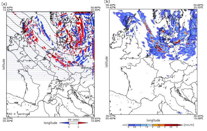
Fig. 4. Cold front on 21 September 2004 at 12:00 UTC. (a) DSI calculated from hourly LM-forecast data on 340 K isentrope (scaled by

standard deviation). Red color indicates positive DSI values and blue negative values. The solid lines show the mean sea level pressure (MSLP). The MSLP data are based on LM-analysis on 21 September 2004 at 12:00 UTC. (b) Total convective precipitation [mm/hr] on 21 September 2004 based on hourly LM-forecast data, 00:00 UTC run + (11–12h). DSI , MSLP and total convective precipitation represent the whole LM domain (325×325 grid points).

summer circulation. Also the mean sea level pressure is dis-played in Fig. 4a, too. The low over Scandinavia can be seen clearly (Fig. 4a). The associated total convective pre-cipitation is shown in Fig. 4b. It must be pointed out, that Fig. 4b shows the hourly accumulated precipitation between 11:00 and 12:00 UTC, whereas the DSI in Fig. 4a displays the snapshot at 12:00 UTC. The synoptic situation was gov-erned by the cyclone QUEEN over northern Europe. The cold front trailing behind this system passed Germany with stormy winds, moving from the Baltic Sea towards the Alps. Behind the postfrontal clearing (subsidence) rain showers developed over northern Germany and Denmark (Fig. 4b). At 12:00 UTC the cold front was above the Alps and over northern Germany a (thermic) trough line was located, which was attenuated while moving southward. Furthermore, there was an incitation of gravity waves and convective cells in the DSI –field in the north-westerly flow over the Scottish Highlands. The cold front is visible as a characteristic dipole structure of the DSI . First an exemplary interpretation of the DSI -pattern and the corresponding total convective pre-cipitation field will be outlined. The quasi-stationary

con-vective line over the North Sea demonstrates a good agree-ment between the DSI and the TC. This system moved only marginally within one hour, towards the south-east with a north-westerly flow direction. The total convective precipita-tion also had this alignment, therefore the one hour accumu-lated rainfall was correctly predicted. The DSI -pattern over middle Germany and the Scottish Highlands shows (Fig. 4a) the trough line at 12:00 UTC moving from the north-west to-wards the east. Therefore the DSI indicates the south-ern boundary of the convective precipitation over Germany and the Scottish Highlands. Now the sign of the DSI shall be discussed. Writing the DSI from Eq. 2 as a scalar triple product, the following form is acquired:

DSI = 1

ρ∇5 · ∇θ × ∇B . (5)

By multiplying Eq. 1 with ρ and the divergence ∇· yields the following equation can be obtained:

∇ · [ρvst] = −

1

52∇5 · ∇θ × ∇B . (6)

(8)

Insertion of Eq. 5 in Eq. 6 the relationship between the divergence and DSI becomes apparent:

∇ · [ρvst] = −

ρDSI

52 . (7)

Hence, the DSI is proportional to the negative divergence, i.e. to the convergence. Positive values (Fig. 4a, red colour, for example over Germany) are connected with a weakening of the PV gradient. The cyclonic flow is also attenuated. In the upper-level at the 340 K isentropic level the is DSI >0, the convergence induced the descent of air masses and hence a weakening of the precipitation intensity. Divergent flow in the upper-level corresponds with negative DSI -values (blue colour) and descending motion can be attributed to the con-vective line over the North Sea. The cyclonic activity is amplified. A band of alternate positive and negative DSI -patterns can be seen over the Baltic Sea. This corresponds with an occlusion front, the low moved eastward. In this region weakening and amplification of the shower-like pre-cipitation fields appeared. The DSI reflects the filament-like structure of the total convective precipitation field. In con-clusion, a weakened PV gradient, associated with positive

DSI -values, indicates a decreased cyclogenesis and

there-fore a lower generation of precipitation and vice versa. 5.3 Correlation between DSI and cloud types

The former two subsections dealt with the link between DSI and precipitation. In this section we concentrate on the clouds, which store the liquid water through the evaporation of water vapour from the surface. Cloud types are not used in numerical forecast models and are also no model-outputs. Only cloud coverage is determined for three different levels. However, the knowledge of cloud types is important for the forecast of precipitation, especially on the convective scale. Based on the cloud types derived from the cloud classifica-tion from Meteosat-8 data at a resoluclassifica-tion of 7 km for the month June, July and August (JJA) 2004, the cloud types were correlated with the |DSI | at the 320 K isentropic level. For this correlation between |DSI | and cloud types values from 09:00 to 16:00 UTC were selected, because the cloud classification uses the visible satellite channels. Cloud types were classified as “rain clouds” and “no rain clouds” accord-ing to Table 1. The cumulus humilis, cumulus fractus and cumulus mediocris are grouped in one class, defined as the cumulus class.

The |DSI |, scaled by the standard deviation, was divided into 26 classes with a bin width of 0.1 in order to gener-ate a class relgener-ated correlation for the above mentioned “rain clouds” and “no rain clouds”. Fig. 5a shows a histogram of the difference of the absolute frequency of no rain clouds and rain clouds for each |DSI |-bin within the period JJA 2004. Clearly a |DSI |-threshold at the class 0.8-0.9 can be seen, where the values change from the positive to the negative range. This result can be used to define a precipitation

activ-Table 1. Cloud types derived from Meteosat-8 and distinguished in

“rain clouds” and “no rain clouds”.

Clouds with rain Clouds without rain

altocumulus/nimbostratus cumulus humilis stratus fractus cumulus fractus cumulonimbus cumulus mediocris cumulus congestus cirrus class cumulus/stratocumulus

ity index of clouds xcpafor each cloud type, which is defined

as:

xcpa=1 −

(x0−xt) − (xt−x∞)

xt ot

. (8) Here, x0−xt denotes the sum of the absolute frequency

for each cloud type between the |DSI | values 0 and 0.9, the

|DSI |-threshold xt is 0.9 , xt−x∞is the sum of all

frequen-cies greater than the threshold and xtot is the absolute

fre-quency of the considered cloud type. With Eq. 8 a hierarchy of dynamical precipitation activity can be established, by cal-culating the index for each cloud type. Fig. 5b shows this new hierarchy together with the simple distribution of the relative frequency of clouds in Fig. 5c. The cumulonimbus cloud has the greatest precipitation activity, followed by the stratus fractus cloud, the cumulus/stratocumulus cloud type, the cumulus congestus cloud, the altocumulus/nimbostratus cloud type. The “no rain cloud” types such as the cumulus humilis, cumulus fractus, cumulus mediocris and especially the cirrus show a significantly lower precipitation activity. In contrast, the absolute frequency of cloud types without dy-namical allocation displays Fig. 5c nearly the reverse range. This important result can be discussed using the example of the cumulonimbus cloud, which has the highest precipitation activity, but the lowest probability of occurrence. This result agrees with the findings of Peters and Christensen (2006), who showed, that rain comes in rare cloudburst rather than as a continuous drizzle. This result of the correlation between clouds and DSI gives the clouds a continuous attribution, which can be used to introduce the cloud information into numerical modelling. In a forecast-mode it is now possible to predict the precipitation activity of different cloud types.

6 Conclusions

The newly designed DSI field variable is a dynamic param-eter, which quantitatively describes the deviation and relative distance from a stationary and adiabatic solution of the prim-itive equations. The DSI , which is calculated from spatial derivatives of basic fields of temperature, velocity and geopo-tential height, is related to non-stationary and diabatic atmo-spheric processes. Thus, the results presented here point out

(9)

(b)

(c)

Fig. 5. (a) Normalised frequency [0_/₀₀_{] of the difference (“no rain clouds” minus “rain clouds”) as a function of |DSI | for JJA 2004 from}

09:00 to 16:00 UTC. The isentropic level is 320 K, representing the middle troposphere. (b) Precipitation activity index of clouds for different cloud types for the period JJA 2004, covering “Central Europe” calculated with Eq. 8. (c) Distribution of the related relative frequency [%] of cloud types. The blue bars in (b) and (c) displays the “rain clouds” and the green bars the “non rain clouds” (see Table 1).

the importance of various non-balanced processes, which dy-namically induce the generation of rainfall. The DSI shows a remarkably high correlation with the precipitation analy-sis of the LM, even without regarding the specific humidity fields. In a case study for frontal systems on the synoptic scale, the DSI reflects the filament-like structure of the

mod-elled total convective precipitation pattern. With the correla-tion between |DSI | and cloud types, derived from Meteosat-8, a threshold can be identified. By using this threshold a precipitation activity index for each cloud type has been cal-culated. This index clearly highlights the infrequently occur-ring cumulonimbus as a high precipitation active cloud type.

(10)

An interesting study would be the analysis of the precipi-tation activity index for different seasons and utilising the COSMO-DE, which has a horizontal resolution of 2.8 km (0.025◦). Besides this the correlation between DSI and pre-cipitation in a forecast mode on a smaller grid of COSMO-DE has also to be investigated further, too. The insights gained from this project may be used for the understanding of precipitation processes and therefore this could be a corner-stone for the improvement of QPF’s.

Acknowledgements. This study is part of the Priority Program SPP 1167 “Quantitative Precipitation Forecast” funded by the German Science Foundation (DFG). We would like to thank T. Schartner for the stimulated discussion and the two anonymous referees for the fruitful comments to improve our manuscript.

Edited by: S. C. Michaelides

Reviewed by: two anonymous referees

References

Banacos, P. C. and Schultz D. M.: The use of moisture flux con-vergence in forecasting convective initiation: historical and op-erational perspectives, Weather and Forecasting, 20, 351–366, 2005.

Berger, F. H.: Die Bestimmung des Einflusses von hohen Wolken auf das Strahlungsfeld und das Klima durch Analyse von NOAA AVHRR-Daten, Ph.D. Thesis, Freie Universit¨at Berlin, Wiss. Met. Abh., Neue Folge Serie A6, 3, 1992.

Doms, G. and Sch¨attler, U.: The nonhydrostatic limit-area model LM (Lokal-Modell) of DWD. Part 1: Scientific Documentation, Deutscher Wetterdienst, Offenbach (available from: http://www. cosmo-model.org), 1999.

Houze, R. A., Jr.: Mesoscale Convective Systems, Rev. Geophysics, 42, RG4003, doi:10.1029/2004RG000150, 2004.

Langer, I. and Reimer, E.: Separation of convective and stratiform precipitation for a precipitation analysis of the local model of the German Weather Service, Adv. Geosci., 10, 159–165, 2007. Langer, I., Reimer, E. and Oestreich, A.: First results: Cloud

classification from Meteosat data for separation of convective and stratiform precipitation, Meteorol. Zeitschrift, 17(1), 29–27, 2008.

Lovejoy, S. and Schertzer, D.: Multifractals and rain, In: New uncertainty concepts in Hydrology and Hydrological modelling, edited by: Z. W. Kundzwewics, 62–103, Cambridge Univ. Press, 1995.

N´evir, P.: Ertel’s vorticity theorems, the particle relabelling symme-try and the energy-vorticity theory of fluid mechanics, Meteorol. Zeitschrift, 13(6), 485–498, 2004.

Olsson, J., Niemczynomicz, J., and Berndtsson, R.: Fractal Analysis of high-resolution rainfall time series, J. Geophys. Res., 98(D12), 23 265–23 274, 1993.

Palm´en, E. and Holopainen, E. O.: Divergence, vertical velocity and conversion between potential and kinetic energy in an extra-tropical disturbance, Geophysica, 8, 89–113, 1962.

Peters, O. and Christensen, K.: Rain viewed as relaxation events, J. Hydrol., 328, 46–55, 2006.

Reimer, E. and Scherer, B.: An operational meteorological diag-nostic system for regional air pollution analysis and long term modelling, In: Air Pollution Modelling and its Application IX, edited by: H. v. Dop, and G. Kallos (Eds.), NATO Challenges of Modern Society, Kluwer Academic/Plenum Publisher, New York, 1992.

Rodriguez-Iturbe, I., Febres de Power, B., Sharifi, M. S., and Geor-gakos, K. P.: Chaos in rainfall, Water Resour. Res., 25(7), 1667– 1675, 1989.

Rose, B. E. J. and Lin, C. A.: Precipitation from vertical motion: a statistical diagnostic scheme, Int. J. Climatol., 23, 903–919, 2003.

Sch¨ar, C.: A generalization of Bernoulli’s theorem, J. Atmos. Sci., 50, 1437–1443, 1993.

Scherhag, R.: Wetteranalyse und Wetterprognose, Springer, Berlin, 1948.

Sivakumar, B.: Is a chaotic multifractal approach for rainfall possi-ble?, Hydrol. Process., 15, 943–955, 2001.

Spar, J.: A suggested technique for quantitative precipitation fore-casting, Mon. Wea. Rev., 81(8), 217–221, 1953.

Tessier, Y., Lovejoy, S., and Schertzer, D.: Universal multifractals: theory and observations for rain and cloud, J. Appl. Meteorol., 32, 223–250, 1993.

Tiedtke, M.: A comprehensive mass flux scheme for cumulus parametrization in large-scale models, Mon. Wea. Rev., 117, 1779–1800, 1989.

Weber, T. and N´evir, P.: Storm tracks and cyclone development using the theoretical concept of the Dynamic State Index (DSI), Tellus A, 60(1), 1–10, doi: 10.1111/j.1600-0870.2007.00272.x, 2008.

Xie, P. and Arkin, P. A.: An intercomparison of gauge observations and satellite estimates of monthly precipitation, J. Appl. Meteo-rol., 34, 1143–1160, 1995.