ÉCOLE DE TECHNOLOGIE SUPÉRIEURE UNIVERSITÉ DU QUÉBEC
AN EXTENDED FINITE ELEMENT-LEVEL SET METHOD FOR SIMULATING TWO-PHASE AND FREE-SURFACE TWO-DIMENSIONAL FLOWS
BY Adil FAHSI
THESIS PRESENTED TO
ÉCOLE DE TECHNOLOGIE SUPÉRIEURE IN PARTIAL FULFILLMENT FOR THE DEGREE
OF DOCTOR OF PHILOSOPHY PH.D.
MONTREAL, SEPTEMBER 9, 2016 Adil Fahsi, 2016
This Creative Commons licence allows readers to download this work and share it with others as long as the author is credited. The content of this work can’t be modified in any way or used commercially.
BOARD OF EXAMINERS
THIS THESIS HAS BEEN EVALUATED BY THE FOLLOWING BOARD OF EXAMINERS
Mr. Azzeddine Soulaimani, Thesis Supervisor
Department of Mechanical Engineering at École de technologie supérieure
Mr. Ammar Kouki, President of the Board of Examiners
Department of Electrical Engineering at École de technologie supérieure
Mr. Stéphane Hallé, Member of the jury
Department of Mechanical Engineering at École de technologie supérieure
Mr. Wahid S. Ghaly, External Evaluator
Department of Mechanical and Industrial Engineering at Concordia University
THIS THESIS WAS PRENSENTED AND DEFENDED
IN THE PRESENCE OF A BOARD OF EXAMINERS AND PUBLIC AUGUST 30, 2016
ACKNOWLEDGMENT
Je tiens à adresser mes remerciements les plus sincères au Professeur Azzeddine Soulaimani qui a bien voulu diriger ces travaux de recherche. Sa solide expérience dans le domaine, sa grande disponibilité et ses conseils éclairés m’ont permis d’apprendre mais surtout de progresser. Puisse-t-il trouver ici l’expression de ma reconnaissance.
Je voudrais également remercier le Professeur Ammar Kouki, pour avoir accepté d’être le président du jury, et les professeurs Stéphane Hallé et Wahid S. Ghaly pour avoir accepté d’évaluer ce travail.
Je remercie chaque membre du groupe de recherche sur les applications numériques en ingénierie et technologie (GRANIT) au sein duquel ces recherches ont été effectuées. Que mes amis et collègues Mamadou, Li, Ali, Imane, Yossera et Ardalan trouvent ici l’expression de ma gratitude.
Je ne saurais oublier l’appui inconditionnel de toute ma famille. Je voudrais remercier en particulier mes parents. Je vous dédie ce travail.
MÉTHODE DES ÉLÉMENTS FINIS ÉTENDUE-LEVEL SET POUR LA SIMULATION DES ÉCOULEMENTS DIPHASIQUES ET À SURFACE LIBRE
Adil FAHSI
RÉSUMÉ
Cette thèse est consacrée à l’étude et au développement de la méthode des éléments finis étendue (XFEM) pour la simulation des écoulements diphasiques. La méthode XFEM est naturellement couplée à la méthode level set pour permettre un traitement efficace et flexible des problèmes contenants des discontinuités et des singularités mobiles. Les équations de Navier-Stokes sont discrétisées en utilisant une paire élément fini stable (Taylor-Hood) sur des maillages triangulaires ou quadrangulaires. Pour la prise en compte des différentes discontinuités à travers l’interface, différents enrichissements de la vitesse et/ou la pression peuvent être utilisés. Cependant, l’ajout de ces enrichissements peut amener à une paire vitesse-pression instable.
Dans ce travail, on considère différents schémas d'enrichissement mixtes, la précision et la stabilité de ces schémas sont étudiées numériquement. Dans un deuxième temps, on s’intéresse à la modélisation de la force de tension superficielle. Cette force engendre un saut dans le champ de pression à travers l'interface. En raison de l’utilisation de la méthode XFEM pour capturer le saut dans la pression, la précision dépend principalement de l’approximation des vecteurs normaux et de la courbure de l’interface. Une nouvelle méthode pour calculer les vecteurs normaux est proposée. Cette méthode utilise des raffinements successifs du maillage à l'intérieur des éléments coupés par l’interface. Ceci permet d'approximer l’interface par des segments linéaires, et les vecteurs normaux construits sont naturellement perpendiculaire à l'interface. Des comparaisons avec des solutions analytiques et numériques montrent que cette méthode est efficace.
La quadrature de la formulation variationnelle des éléments coupés par l’interface est améliorée en utilisant une subdivision récursive. La réinitialisation du level set est réalisée par une approche directe basée sur un raffinement de maillage afin de préserver la propriété de la distance signée de la fonction level set. Les méthodes proposées sont testées et validées sur des tests numériques de complexité croissante: écoulement de Poiseuille diphasique, écoulement extensionnel, réservoir rectangulaire soumis à une accélération horizontale, sloshing dans un réservoir, effondrement d’une colonne d'eau avec et sans obstacle, et bulle montante dans un récipient d'eau. Pour tous les régimes d'écoulement, nos résultats sont en bon accord avec soit des solutions analytiques ou des données de références expérimentales ou numériques.
Mots-clés: écoulement diphasique incompressible; méthode des éléments finis étendue; enrichissements de la vitesse et de la pression; condition inf-sup; tension superficielle; écoulement à surface libre
AN EXTENDED FINITE ELEMENT-LEVEL SET METHOD FOR SIMULATING TWO-PHASE AND FREE-SURFACE TWO-DIMENSIONAL FLOWS
Adil FAHSI ABSTRACT
The present work discusses the application of the extended finite element method (XFEM) to model two-phase flows. The XFEM method is naturally coupled with the level set method to provide an efficient and flexible treatment of problems involving moving discontinuities. The Navier-Stokes equations are discretized using a stable finite element pair (Taylor-Hood) on triangular or quadrangular meshes. In order to account for the discontinuities in the field variables across the interface, kink or jump enrichments may be used for the velocity and/or pressure fields. However, these enrichments may lead to an unstable velocity-pressure pair. In this work, different enrichment schemes are considered, and their accuracy and stability are numerically investigated. In cases with a surface tension force, a jump in the pressure field exists across the moving interface. Because we employ the XFEM to capture this jump, the accuracy mainly relies on the precise computation of the normal vectors and the curvature. A novel method of computing the vectors normal to the interface is proposed. This method computes the vectors normal by employing the successive refinement of the mesh inside the cut elements. This provides a high resolution of the interface position. The normal vectors thus constructed are naturally perpendicular to the interface. Comparisons with analytical and numerical solutions demonstrate that the method is effective.
The quadrature of the Galerkin weak form for the intersected elements is improved by employing a mesh refinement. The reinitialization of the level set field is realized by a direct approach in order to recover the signed-distance property. The proposed methods are tested and validated for various numerical examples of increasing complexity: Poiseuille two-phase flow, extensional flow problem, a rectangular tank in a horizontal acceleration, sloshing flow in a tank, a collapsing water column with and without obstacle, and a rising bubble. For all flow regimes, excellent agreement with either analytical solutions or experimental and numerical reference data is shown.
Keywords: incompressible two-phase flow; extended finite element method; velocity and pressure enrichments; inf-sup condition; surface tension; free surface flows
TABLE OF CONTENTS
Page
INTRODUCTION ...1
CHAPTER 1 GOUVERNING EQUATIONS OF TWO-FLUID FLOWS ...11
Incompressible Navier-Stokes equations ...11
1.1.1 Boundary, interface and initial conditions ... 13
Interface description for two-phase fluid flows ...16
1.2.1 Description of the level set ... 16
Closure ...19
CHAPTER 2 THE EXTENDED FINITE ELEMENT METHOD (XFEM) ...21
A literature review of the XFEM ...21
2.1.1 Coupling XFEM with the level set ... 24
2.1.2 Applications ... 24
The XFEM formulation ...25
2.2.1 Modeling strong discontinuities ... 27
2.2.2 Modeling weak discontinuities ... 31
Example: One dimension bi-material bar ...35
Closure ...38
CHAPTER 3 SPACE AND TIME DISCRETIZATIONS...39
Derivation of the weak formulation of the Navier-Stokes equations ...39
Time discretization of the Navier-Stokes equations ...42
Strategies for numerical integrations ...45
3.3.1 Decomposition of elements ... 45
3.3.2 Linear dependence and ill-conditioning ... 48
3.3.3 Time-Stepping in the XFEM ... 49
Derivation of the weak formulation of the level set transport equation ...50
Level set update and reinitialization ...51
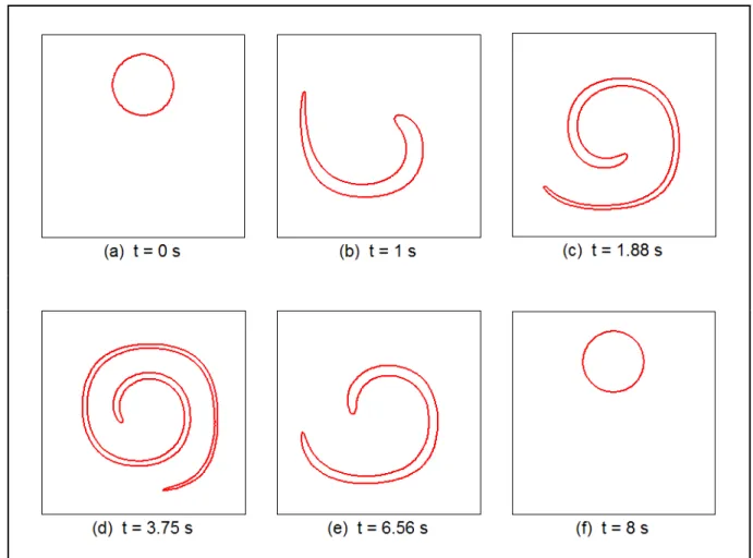
3.5.1 Numerical example: Vortex in a box ... 51
3.5.2 Reinitialization ... 55
Inf-sup stability issue with XFEM ...57
Closure ...59
CHAPTER 4 NUMERICAL SIMULATION OF SURFACE TENSION EFFECTS ...61
Numerical computation of normal and curvature ...61
4.1.1 L2-projection method... 62
4.1.2 Geometric method: Closest point on the interpolated interface ... 64
Comparison: Spatial convergence...69
Comparison: Moving interface ...74
CHAPTER 5 SOLUTION PROCEDURE ...79
XII
Time step size limit ... 81
The Navier-Stokes/level set coupling algorithm ... 82
CHAPTER 6 NUMERICAL TESTS ... 85
Stationary straight interface ... 86
6.1.1 Poiseuille two-phase flow ... 86
6.1.2 Extensional flow problem ... 97
Numerical examples: A moving interface ... 103
6.2.1 Rectangular tank under horizontal acceleration ... 103
6.2.2 Sloshing flow in a tank ... 109
6.2.2.1 Comparison of 0 P R− ×1 and 0 P sign− ×1 enrichment... 112
6.2.3 Dam break problem ... 114
6.2.4 Dam break with an obstacle ... 118
6.2.5 Bubble rising in a container fully filled with water ... 121
CONCLUSION ... 131
LIST OF TABLES
Page
Table 6-1 XFEM approximations and their abbreviations ...88 Table 6-2 Errors of the interface slope for different enrichments ...105 Table 6-3 Physical properties and dimensionless numbers defining test case ...122 Table 6-4 Collected data from simulations and reference values observed in
simulations by (Hysing, Turek et al. 2009) ...127 Table 6-5 Mass errors for rising bubble at t =3 s ...129
LIST OF FIGURES
Page
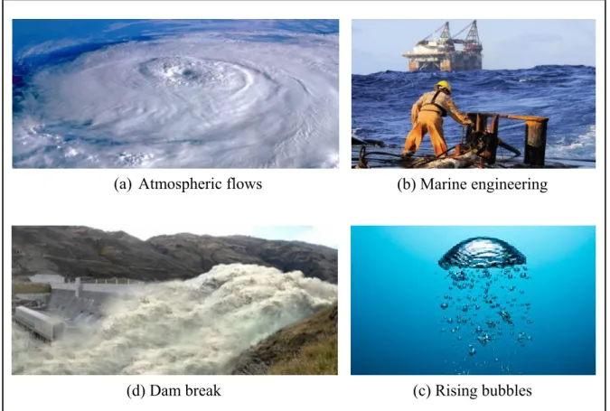
Figure 0.1 Examples of immiscible fluids in industrial and natural processes ...1
Figure 0.2 Kink and jump discontinuities ...3
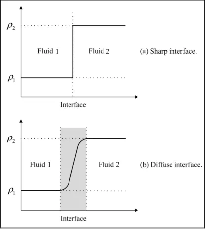
Figure 0.3 Schematic picture of a classical sharp interface and a diffuse interface ...4
Figure 0.4 Jump in the pressure field ...7
Figure 1.1 Two immiscible fluids Ω1 and Ω2 separated by the interface Γint ...11
Figure 1.2 Two-phase flow discontinuities: (a) viscosity jump, (b) density jump, and (c) surface tension ...15
Figure 1.3 Definition of level set function ...17
Figure 1.4 A circular interface in 2D (a) represented by the signed distance function φ (b) ...18
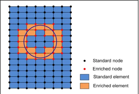
Figure 2.1 Domain with a circular interface illustrating the set of enriched nodes and the enriched elements ...26
Figure 2.2 Problem statement ...28
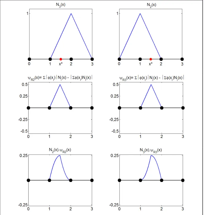
Figure 2.3 Enriched basis function for a strong discontinuity in 1D ...30
Figure 2.4 Enriched basis function for a weak discontinuity in 1D ...32
Figure 2.5 Enriched basis function for modified abs-enrichment (Moës, Cloirec et al. 2003) for a weak discontinuity in 1D ...34
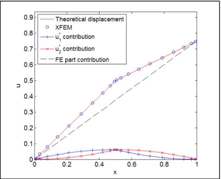
Figure 2.6 Bi-material rod in traction ...35
Figure 2.7 XFEM and FEM solutions of the bi-material rod ...37
Figure 2.8 XFEM solution with 1 element and modified abs-enrichment function ....37
Figure 3.1 Elements used in this work ...42
Figure 3.2 Sub-elements and integration points. Red line depicts the interface, and blue points depict the nodes ...46
XVI
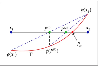
Figure 3.3 Curved interface inside a quadratic element and integration error committed with the linear approximation of the interface. In green, the
approximated interface and computed points Pi on the interface ... 47
Figure 3.4 Estimation of the iso-zero level set position. In blue, grid points ... 47
Figure 3.5 An interface passing close to a vertex (left) or edge (right) ... 48
Figure 3.6 Time evolution of the iso-zero level set for the vortex in a box ... 53
Figure 3.7 Comparison of the final shape of the iso-zero level set for the vortex in a box. The initial shape of the disk is taken as a reference ... 54
Figure 3.8 Area of the disk over time t ... 54
Figure 3.9 Example of recursive subdivision of level 4 to localize a circular interface. In black, the initial mesh. In blue, the refined mesh ... 56
Figure 3.10 Reinitialization of the level set function using a recursive subdivision of level 4: (a) before the reinitialization; (b) after the reinitialization ... 57
Figure 4.1 Example of recursive subdivisions of different levels to localize the interface. Red curve depicts the exact interface, and green points depict the iso-zeros level set ... 65
Figure 4.2 A quadratic element ... 66
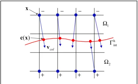
Figure 4.3 Closest point. Blue dots are grid points with their corresponding closest point c x( ) on the interface as red dots. Collinear vectors ( ) col v x are drawn from xc x( ). ”+ ” and ” − ” indicate the signs of the level set nodal values ... 68
Figure 4.4 Projection of the tangential unit vector tint. The normal unit vector int n is then computed using (4.17); the segments Si are in red and the iso-zeros level set Pi are in green ... 68
Figure 4.5 Computational domain for the static disc test case ... 70
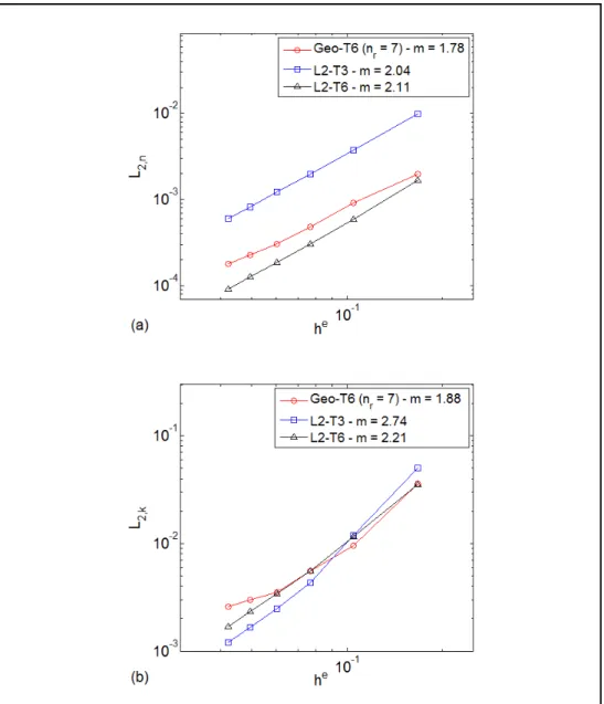
Figure 4.6 Stationary circular bubble: convergence study, L2−norm of the error on the normal (a) and curvature (b). We compare the two following methods on structured meshes: The geometrical method (
Geo
−
T6
) and the L2 projection− method using a linear element (L
2 T3
−
) and a quadratic element (L
2 T6
−
) ... 72Figure 4.7 Stationary circular bubble: convergence study of the
Geo
−
T6
methodfor different levels of refinement nr ...74
Figure 4.8 Moving circular bubble: initial configuration ...75
Figure 4.9 Moving circular bubble: convergence study at t =1 s, L2 −norm of the error on the normal (a) and curvature (b) and convergence rates (m) ...76
Figure 5.1 Flowchart for weak coupling between Navier-Stokes and level set transport equations ...80
Figure 6.1 Two-phase Poiseuille: computational domain and mesh, with he =0.05 ...86
Figure 6.2 Two-phase Poiseuille: the P1−P1 enrichment performs better than the 1 0 P− and P2−P1 enrichments. The horizontal velocity is evaluated at the Gauss points of each element ...89
Figure 6.3 Two-phase Poiseuille: convergence study for the different enrichment schemes ...90
Figure 6.4 Two-phase Poiseuille: evolution of the numerical inf-sup β ...93h Figure 6.5 Position of the interface across elements ...94
Figure 6.6 Minimum element area ratio Amin ...95
Figure 6.7 Two-phase Poiseuille: influence of an ill-conditioned system ...96
Figure 6.8 Extensional flow problem: computational mesh, with he =0.091 ...98
Figure 6.9 Extensional flow problem with jump in the viscosity: convergence study, L2−norm of the error in the pressure field and convergence rates (m) ...98
Figure 6.10 Extensional flow problem with jump in the viscosity: pressure field ...99
Figure 6.11 Extensional flow problem with jump in the viscosity: comparison of the pressure field section at
x
=
0.5
...100Figure 6.12 Extensional flow problem with jump in the viscosity and discontinuous volume force: convergence study, L2−norm of the error in the pressure field ...101
XVIII
Figure 6.13 Extensional flow problem with jump in the viscosity and
discontinuous volume force: pressure fields for the sign function (left) and the ridge function (right) ... 102 Figure 6.14 Tank under horizontal acceleration: initial configuration and
computational mesh, he =0.016 ... 104
Figure 6.15 Tank under horizontal acceleration: free surface for different
enrichments ... 106 Figure 6.16 Parasite velocities: the ∅ − P1 enrichment (a) performs better than
the P1 − P1 (b) and the P2 − P1 (c) enrichments ... 107 Figure 6.17 Numerical smoothing region ... 108 Figure 6.18 Sloshing tank: initial configuration and computational mesh, with
he ≈0.015 ... 110
Figure 6.19 Sloshing tank: interface position and velocity solution in m / s for various time instances ... 111 Figure 6.20 Sloshing tank: interface height at the right side wall ... 112 Figure 6.21 Sloshing tank: comparison of snapshots of the velocity field at
t 1.20 s= ... 112 Figure 6.22 Sloshing tank: mass conservation for t∈
[
0, 6 s]
... 113 Figure 6.23 Sloshing tank: comparison of mass conservation using nr =0 andnr =1 for the numerical integration ... 114 Figure 6.24 Dam break problem: initial configuration ... 115 Figure 6.25 Dam break problem: Dimensionless width x aw/ (i) and height
/(2 )
w
y a (ii) as a function of time, comparison with experimental data from (Martin and Moyce 1952) ... 116 Figure 6.26 Dam break problem: comparison of the numerical and experimental
(Koshizuka, Tamako et al. 1995) free surfaces ... 117 Figure 6.27 Dam break with an obstacle: initial configuration ... 119 Figure 6.28 Dam break with an obstacle: comparison of the numerical and
Figure 6.29 Rising bubble: initial configuration ...122 Figure 6.30 Rising bubble: snapshots of the three computational meshes.
(a) 1280 elements; (b) 2508 elements; (c) 4781 elements ...124 Figure 6.31 Rising bubble: pressure solution in N/m2 and interface position for
various time instances ...125 Figure 6.32 Rising bubble: temporal evolution of (a) center of mass position
and (b) rising velocity. Comparison of the results with simulation data from (Hysing, Turek et al. 2009) ...126 Figure 6.33 Rising bubble: final shape of the bubble at t=3 s and reference
solution by Hysing et al. (Hysing, Turek et al. 2009) ...128 Figure 6.34 Rising bubble: mass errors at t=3 s ...129
LIST OF ABREVIATIONS
ALE Arbitrary Lagrangien-Eulerien
BB Babuska-Brezzi condition
BDF Backward Differentiation Formula CFD Computational Fluid Dynamics CSF Continuum Surface Force method
CFL Courant-Freidrichs-Lewy number
Dof Degrees of freedom FEM Finite Element Method
FSI Fluid-Structure Interaction problems GFEM Generalized Finite Element Method GLS Galerkin/Least-Squares LEFM Linear Elastic Fracture Mechanics
LS Level Set
MLPG Meshless Local Petrov-Galerkin QUAD Quadrangle
RK Runge-Kutta time integration PDE Partial Differential Equation PUM Partition of Unity property
SPH Smoothed Particle Hydrodynamics SSP Strong-Stability Preserving SUPG Streamline/Upwind Petrov-Galerkin TRI Triangle
VMS Variational Multiscale method
VOF Volume-of-Fluid method
LIST OF SYMBOLS
abs( )⋅ absolute value function
( )
A⋅ area of specified domain
α interface thickness h β stability coefficient C convective matrix corr ( )⋅ corrected value ε
δ Dirac delta function ij
δ Kronecker symbol
D
( )⋅ Direchlet boundary value γ surface tension coefficient
∇ continuous gradient operator
∇ ⋅ continuous divergence operator D Γ Dirichlet boundary N Γ Neumann boundary int Γ Interface ( )u
ε rate of deformation tensor κ curvature
μ dynamic viscosity
v kinematic viscosity
ρ density
( , )u p
σ Cauchy stress tensor L
τ stabilization parameter of SUPG term of level set equation
φ level set function
Ω domain ∂Ω domain boundary e Ω element domain e element ⋅ Euclidean norm ( )⋅ ex exact value Eo Eötvös number
I set of all nodes
*
I set of enriched nodes 0
( )⋅ initial value
f right-hand-side vector
f frequency
ST
f surface tension force vector g magnitude of gravity force vector
XXIV
g gravity force vector
Hα Heaviside function
G gradient matrix
ψ global enrichment function
he
characteristic element length 1( )
H Ω Sobolev space of square-integrable functions with square-integrable first derivatives
i node
( )⋅ i nodal value
I identity tensor
⋅ jump operator( )⋅ k identifier for fluid in two-phase flow
K viscous matrix
max
( )⋅ maximal value
min
( )⋅ minimal value
M local enrichment function
M mass matrix
n number of degrees of freedom
n number of space dimensions el
n number of elements
ns number of sampling time steps r
n level of mesh refinement num
( )⋅ numerical value
n outer unit normal vector on domain boundary int
n unit normal vector on interface int, int
x y
n n first and second components of the normal unit vector
N shape function
N matrix containing shape functions
N matrix containing shape and enrichment functions 2( )
L Ω Hilbert space of square-integrable functions
p pressure
P vector of pressure degrees of freedom i
P iso-zero level set position q pressure weighting function
r radius ref ( )⋅ reference value * ( )⋅ related to enrichment Re Reynolds number
S slope p
S solution function space for pressure Su solution function space for velocity
Sφ solution function space for level set δ smaller distance to interface
t time T period end t time period t Δ time-step length int
t unit tangential vector on interface int, int
x y
t t first and second components of the tangential unit vector t
∂ time derivative
u velocity vector
u velocity vector along x−axis
n
u normal component of the velocity at the interface U vector of velocity degrees of freedom
υ
velocity vector along y−axis v velocity weighting functionx
v velocity weighting function (for u) y
v velocity weighting function (for
υ
)( )
V ⋅ volume of specified domain p
V weighting function space for pressure Vu weighting function space for velocity
Vφ weighting function space for level set i
j
ω weights of the Q−point Gauss quadrature
w level set weighting function G
x center of mass
G, G
x y first and second coordinate of center of mass
x coordinate vector
,
x y first (horizontal) and second (vertical) coordinate i
j
INTRODUCTION
Multi-phase flow simulation is an indispensable tool for controlling and predicting physical phenomena in a wide range of engineering and industrial systems, e.g., aerospace, chemical, biomedical, ship hydrodynamics, hydraulic design of dams, nuclear and naval engineering. The main numerical modeling difficulties are due to the jumps in fluid properties (density and viscosity) across the interface, the discontinuities of the flow variables across the interface, the surface tension force that introduces a jump in the pressure field, the changes in the topology of the interface as it evolves with time, and the time and space multi-scales that can exist in the physical phenomena.
Figure 0.1 Examples of immiscible fluids in industrial and natural processes
In two-fluid flow simulations, it is known that unphysical currents or spurious velocities may occur in fluid regions adjacent to an interface (Ganesan, Matthies et al. 2007; Zahedi,
(a) Atmospheric flows (b) Marine engineering
(c) Rising bubbles (d) Dam break
2
Kronbichler et al. 2012). Their magnitude depends on various factors, such as, the approximation of the pressure jump across the interface, the approximation of the normal vectors to the interface and the curvature required for the calculation of the surface tension force. Spurious velocities may affect the prediction of flow field velocities, or, in more extreme circumstances, can cause the complete break-up of an interface. Therefore, the minimization of such unphysical currents is highly desirable.
Numerous methods have been developed for handling incompressible two-fluid flows. The main difference between them methods is how the interface is represented. All methods can be divided into two general groups:
• interface-tracking methods or moving mesh: front tracking methods (Unverdi and Tryggvason 1992), arbitrary Eulerian-Lagrangian methods (ALE) (Huerta and Liu 1988), boundary integral methods (Best 1993), and deforming space-time finite element formulations (Tezduyar, Behr et al. 1992; Tezduyar, Behr et al. 1992). These methods are accurate for rigid moving boundaries, but the re-meshing procedure can fail when the interface topology is significantly altered; and
• interface-capturing methods or fixed mesh: volume of fluid methods (VOF) (Hirt and Nichols 1981; Pilliod Jr and Puckett 2004), level set methods (Osher and Sethian 1988; Sussman, Smereka et al. 1994; Sethian 1999), and diffuse interface methods (Verschueren, Van De Vosse et al. 2001). These methods are more convenient when large deformations occur at the interface, but they require a higher mesh resolution.
Interface-tracking methods offer an accurate description of the interface and thereby conserve masses (volumes) quite well. In the case of topological changes, which are encountered in immiscible multi-phase flows, these methods are inconvenient and induce significant loss of accuracy, especially when frequent re-meshing is necessary. The challenge associated with the interface-tracking approaches is to address significant topological changes, such as stretching, tearing or merging of configurations. In contrast, the interface-capturing methods are naturally able to account for topological changes of the interface between fluids. This allows for a flexible interface description compared to the interface-tracking methods, but
they are often less accurate, e.g., in terms of mass conservation. To increase the accuracy, a mesh refinement is often used close to the interface.
The level set method, introduced by Osher and Sethian (Osher and Sethian 1988), is a popular approach for describing the interface motion in two-phase fluid flows (Sussman, Smereka et al. 1994; Sussman, Fatemi et al. 1998) because it can efficiently handle rapid topological changes as well as the splitting and merging of fluids. Owing to the implicit capture of the interface, some elements may be cut by the interface, and discontinuities therefore occur inside them. Strong and weak discontinuities are encountered. Problems with strong discontinuities present a jump in the solution field, whereas for weak discontinuities, the solution field is continuous and shows a kink, and a jump appears in the derivative of the solution field.
Figure 0.2 Kink and jump discontinuities
Using a standard finite element method (FEM), the jumps and kinks in the pressure and velocity fields across the interface cannot be represented explicitly (Gross and Reusken 2011). To overcome this problem, we can use the diffuse interface method. The viscosity and density can be regularized such that instead of jumping discontinuously, they go smoothly from
ρ
1 toρ
2 (μ
1 toμ
2) over several elements, see Figure 0.3.4 1 ρ 2 ρ 1 ρ 2 ρ
Figure 0.3 Schematic picture of a classical sharp interface and a diffuse interface
However, such approaches may introduce unphysical diffusive effects (Smolianski 2001). The extended finite element method (XFEM) originally developed for crack problems by Belytschko and Black (Belytschko and Black 1999) and redefined by Moës et al. (Moës, Dolbow et al. 1999) addresses these difficulties by enriching the approximation space to represent a known type of discontinuity in the element interiors. XFEM utilizes the partition of unity property (PUM) of the finite element shape functions (Melenk and Babuška 1996). The XFEM popularity is observed because a non-adapted mesh could be used, and the laborious re-meshing procedures are no longer necessary.
Owing to the PUM, strong discontinuities can be accurately reproduced by the sign of the level set function or the jump enrichment (Dolbow, Moës et al. 2000), and the optimal convergence rate can be obtained upon mesh refinement. A weak discontinuity can be
incorporated by the absolute value of the level set function (abs-enrichment or kink enrichment); one alternative proposed by Moës et al. (Moës, Cloirec et al. 2003) is the modified abs-enrichment. These enrichments were initially applied to solid mechanics problems.
In two-phase fluid flows, various enrichment schemes for the velocity and/or pressure can be imagined. Chessa and Belytschko (Chessa and Belytschko 2003; Chessa and Belytschko 2003) applied the standard abs-enrichment to account for kinks in the velocity field but did not enrich the pressure field for problems with and without surface tension effects. In addition to the kink enrichment of the velocity field, Minev et al. (Minev, Chen et al. 2003) employed a jump enrichment of the pressure field due to the presence of surface tension effects. In contrast, Groß and Reusken (Groß and Reusken 2007) used Heaviside enrichment to enrich the pressure field for 3D two-phase flows with surface tension effects, but they did not enrich the velocity field. Zlotnik and Díez (Zlotnik and Díez 2009) generalized the modified abs-enrichment (Moës, Cloirec et al. 2003) for n−phase flow (n>2), in which different interfaces intersect an element. They enriched the velocity and pressure fields in the case of quasi-static Stokes flow problems. Fries (Fries 2009) used the intrinsic XFEM and performed the enrichment of both the velocity and pressure fields for two-phase flow problems with surface tension effects. Cheng and Fries (Cheng and Fries 2012) developed the h-version of XFEM and used sign enrichment to account for the jump and/or kink in the pressure field in 2D and 3D two-phase incompressible flows. Sauerland and Fries (Sauerland and Fries 2011; Sauerland 2013) suggested the use of sign enrichment to enrich the pressure as a means to represent weak and strong pressure discontinuities, but not for the velocity; they reported that enriching the velocity does not significantly improve the results, and in some cases of unsteady flows, the convergence problems were so severe that no convergence was achieved (Liao and Zhuang 2012). Recently, several XFEM enrichments, following a similar approach to reproduce the internal discontinuities of two-phase flows, were proposed, e.g., by Ausas et al. (Ausas, Buscaglia et al. 2012) and Wu and Li (Wu and Li 2015).
6
The issue of the discretization of the incompressible Navier-Stokes equations is an important aspect of one-phase and two-phase flow modelling. The approximation spaces of velocity and pressure must satisfy the inf-sup stability condition (LBB) to avoid spurious pressure modes in the numerical solution. There are two strategies for dealing with the LBB condition: (i) satisfying it by choosing an appropriate velocity-pressure element pair, where interpolants of one order lower than those of the velocity are used for the pressure interpolation and (ii) avoiding it by stabilizing the discretized weak formulation. The stabilization enables the use of equal-order interpolation for the pressure and velocity fields. Using numerical experiments, Legrain et al. (Legrain, Moës et al. 2008) analysed the stability of incompressible formulations in elasticity problems enriched with XFEM. They concentrated on the application of XFEM to mixed formulations for problems with fixed interfaces such as the treatment of material inclusions, holes and cracks. In two-phase flows, Groß and Reusken (Groß and Reusken 2007) refine the mesh close to the interface and modify the Taylor-Hood element (P2/P1) by enriching the pressure with discontinuous approximations (P1/P0 enrichment). They proved the optimal error bounds for the P1/P0
approximation, but the inf-sup stability and the order of convergence issue was not investigated numerically or theoretically; it remains an open problem (Esser, Grande et al. 2010). Sauerland and Fries (Sauerland and Fries 2011; Sauerland 2013) numerically investigated different enrichment strategies for two-phase and free-surface flows, utilizing a stabilized Galerkin-Least-Squares (GLS) formulation because the basic interpolations for the velocity and the pressure are of equal order (Q1/Q1). However, the stability of these strategies was not shown.
The modeling of the surface tension force presents another difficult task in two-phase flows and remains a challenge for two reasons. The first is that it requires the computation of the normal and surface curvatures of the interface, i.e., first and second derivatives of the level set function. The second difficulty is that the surface tension is applied on the interface, which is not straightforward to realize in the case of an implicit interface representation, i.e., in the context of the level set function, on a surface embedded in the mesh. Yet, one possibility is to convert the surface tension force into a volume force employing the
continuum surface force method (CSF) (Brackbill, Kothe et al. 1992). Thereby, the pressure jump is smoothed across a certain distance ε instead of being treated accurately (see Figure 0.4). The focus of this work lies on a sharp interface representation and on the XFEM to capture the discontinuities within elements by enriching the approximation space.
Figure 0.4 Jump in the pressure field
The present research has two objectives. First, we analyze different enrichment schemes of velocity and/or pressure fields, and their accuracy and stability are numerically investigated for test cases involving weak and/or strong discontinuities. We advocate the use of Taylor-Hood mixed interpolations (P2/P1 or Q2/Q1) as the basic element; they have been proven to be robust and more stable even at large Reynolds numbers (Arnold, Brezzi et al. 1984). Second, we present a novel approach for computing the vectors normal to the interface, which are indispensable for the calculation of the curvature and surface tension force. In this approach, a multi-level mesh refinement is first realized inside cut elements, and the points on the interface with a zero level set in each sub-element are then computed; those points are connected with straight segments Si that are stored. Finally, the vectors normal to the piecewise linear interface are constructed. Thereby, the normal vectors are perfectly perpendicular to the interpolated interface. We analyze the accuracy of the approach, first on a geometric case and then on the complex simulation of the bubble rise problem.
8
The thesis is divided into six chapters. In the first one, we give an introduction to two-fluid flow modelling together with the motivation for the present study. Chapter 1 introduces the governing Navier-Stokes and the level set transport equations. The equations are accompanied by initial, boundary, and interfacial conditions for the two-fluid interface. Chapter 2 presents the extended finite element method (XFEM) for the spatial discretization. Different enrichment schemes for two-phase flows are discussed. Chapter 3 considers the following aspects: (a) derivation of the weak formulation of the incompressible Stokes equations and the level-set transport equation, (b) time discretization of the Navier-Stokes equations, (c) strategies for numerical integration, (d) level set updating and reinitialization, and (e) the inf-sup stability issue with XFEM. The following chapter deals with the modelling of surface tension. This is followed by a discussion on the construction of the vectors normal to the interface. Chapter 5 describes in detail the coupling between the Navier-Stokes equations and level set equation with accompanying flowchart. Furthermore, we highlight the time-step size limit. Numerical results for several test cases are presented in Chapter 6. Finally, the thesis is summarized, and the main conclusions and suggestions for future research are presented.
Publications related to this thesis
The results presented in this thesis have led to the following publications in international journals:
Fahsi, A. and A. Soulaimani (Submitted 2016). "Numerical investigations of the XFEM for solving two-phase incompressible flows." International Journal for Numerical Methods in Fluids FLD-16-0243.
Touré, M. K., A. Fahsi, et al. (2016). "Stabilised finite-element methods for solving the level set equation with mass conservation." International Journal of Computational Fluid Dynamics 30(1): 38-55.
Fahsi, A. and A. Soulaïmani (2011). The extended finite element method for moving interface problems. AÉRO 11, 58th Aeronautics Conference and AGM. Sustainable Aerospace: The Canadian Contribution, Montréal, QC, Canada, Apr. 26-28.
Fahsi, A. and A. Soulaïmani (2013). Velocity-Pressure enrichments for the Taylor-Hood elements for solving moving interface two-phase flows. Annual Meeting of the Canadian Applied and Industrial Mathematics Society CAIMS 2013, Quebec City, QC, Canada, June 16-20.
Soulaïmani, A., A. Fahsi, et al. (2013). A computational approach in XFEM for two-phase incompressible flows. Advances in Computational Mechanics (ACM 2013) - A Conference Celebrating the 70th Birthday of Thomas J.R. Hughes, San Diego, CA, USA, Feb. 24-27.
Soulaïmani, A., A. Fahsi, et al. (2014). Extended velocity-pressure for solving moving interface two-phase flows. 11th World Congres on Computational Mechanics, WCCM XI, Barcelona, Spain, July 20-25.
CHAPTER 1
GOUVERNING EQUATIONS OF TWO-FLUID FLOWS
The governing incompressible Navier-Stokes and the level set transport equations are detailed in this chapter. Those equations are accompanied by initial, boundary, and interfacial conditions. The chapter also describe the possible discontinuities across the interface of the flow variables.
Incompressible Navier-Stokes equations
The domains occupied by two or more immiscible fluids are denoted by Ωk, with Ω = ∪Ωk the computational domain and Γ its boundary (cf. Figure 1.1). The interface separating the phases is denoted by Γint, with the normal vector nint.
2
Ω
1Ω
NΓ
intn
Γn
Γ
intΓ
D ΓFigure 1.1 Two immiscible fluids Ω1 and 2
Ω separated by the interface Γint
The fluid density ρ and viscosity μ are functions of position and time, so that
1 1 2 2 if ( ) ( , ) if ( ) t t t ρ ρ ρ ρ ∈ Ω = = ∈ Ω x x x (1.1)
12 1 1 2 2 if ( ) ( , ) if ( ) t t t μ μ μ μ ∈ Ω = = ∈ Ω x x x (1.2)
We only consider two-dimensional spatial domains in this thesis. For each phase k , the Navier-Stokes equations governing the incompressible Newtonian flows are written as
(
2 ( ))
( , int) ST, k p k k t ρ ∂ + ⋅∇ = −∇ + ∇⋅ μ +ρ +δ Γ ∂ u u u ε u g x f (1.3)0.
∇⋅ =
u
(1.4) or in component notation int ST 2 ( , ) k k k k x x u u u p u u u g f t x y x x x y y x υ ρ ∂∂ + ∂∂ +υ∂∂ = −∂∂ +∂∂ μ ∂∂ +∂∂ μ ∂∂ +∂∂ +ρ +δ Γ x int ST 2 ( , ) k k k k y y p u u g f t x y y x y x y y υ υ υ υ υ ρ ∂∂ + ∂∂ +υ∂∂ = −∂∂ +∂∂ μ ∂∂ +∂∂ +∂∂ μ ∂∂ +ρ +δ Γ x 0 u x y υ ∂ +∂ = ∂ ∂where (1.3) denotes the momentum equations and (1.4) the continuity equation (incompressibility constraint), u=( , )u υ T the fluid velocity vector, t the time, p the dynamic pressure, g the gravitational acceleration, ε( )u the rate of deformation tensor
T 1
2
( )u = (∇ + ∇u ( u) )
ε (1.5)
ST( )=γ κ int
f x n (1.6)
where γ is the surface tension coefficient in the normal direction,
κ
is the interfacial curvature, δ( ,xΓint) is the Dirac delta function, and Γint is the interface line (surface in 3D).1.1.1 Boundary, interface and initial conditions
In order to obtain a well-posed problem, boundary conditions have to be imposed on the external boundary Γ and on the interface. The Dirichlet and Neumann boundary conditions are prescribed as D, D = ∀ ∈ Γ u u x (1.7) N , Γ ⋅n =h ∀ ∈ Γx σ (1.8)
where ΓD denotes the Dirichlet boundary, ΓN the Neumann boundary, uD and h the specified velocity and stress, respectively, σ( , )u p = −pI+2μkε( )u the Cauchy stress tensor,
Γ
n the outward pointing normal vector on the boundary Γ , and I the identity tensor.
The interfacial equilibrium conditions, which couple the stress and velocity between the two phases at the interface, are given by
u =uΩ1−uΩ2 = 0, ∀ ∈ Γx int,t∈[
0,tend]
(1.9)14
where the operator
• represents the jump across the interface Γint. It can be seen from the equilibrium condition of the interfacial force (1.10) that the total stress generated by two-phase flow is balanced with the surface tension.Initial conditions complement the problem as indicated:
0
( , 0)= ( ), ∀ ∈ Ω at t=0
u x u x x (1.11)
Inserting the definitions for stress and strain tensors into the interface condition for the normal stress (1.10) results in
(
T)
[
]
int int int end
( ) , , 0, p μ γ κ t t − + ∇ + ∇I u u ⋅n = n ∀ ∈Γx ∈ (1.12)
It is clear that the presence of the viscosity jump or/and the surface tension at the interface leads to a jump in the pressure field and a jump in the velocity gradient across the interface. In the hydrostatic case (
u 0
=
) and without surface tension (γ =0), the momentum equation in (1.3) reduces to[
end]
, , 0, k k p ρ t t ∇ = g ∀ ∈ Ωx ∈ (1.13)Along the interface, Eq. (1.13) can be written as
∇ =p ρ g, ∀ ∈Γx int,t∈[
0,tend]
(1.14) We note that the gravitational forces in combination with a jump in the density lead to a jumpin the pressure gradient.
In the numerical simulation of incompressible immiscible two-phase flows, we need to account for
• a jump in the gradient velocity (or kink in the velocity) across the interface where viscosity jumps exist (cf. Figure 1.2a);
• a jump in the pressure where viscosity jumps or/and surface tension exist (cf. Figure 1.2a and Figure 1.2c); and
• a jump in the gradient pressure (or kink in the pressure) where density jumps exist (cf. Figure 1.2b). 1 μ 2 μ u p 1 ρ 2 ρ p g γ p
Figure 1.2 Two-phase flow discontinuities: (a) viscosity jump, (b) density jump, and (c) surface tension
16
Interface description for two-phase fluid flows
In this section, we introduce the level set method as a method for the implicit representation of interfaces. The level set method (Osher and Sethian 1988) is a numerical technique originally developed to analyze and follow the motions and deformations of an interface under an arbitrary velocity field. This velocity can depend: on the position of the interface, on time, on a related underlying physical problem, on a geometrical property of the interface or on any other parameters. Osher and Sethian proposed to introduce a smooth scalar function φ( )x defined on all x ∈ n which, at all times, should represent an interface Γint of dimension n 1− as the set where φ( ) 0x = .
Up to now, this method has been successfully applied to numerous physical problems: multi-phase fluid flows (Sussman, Smereka et al. 1994), crack propagation (Strouboulis, Babuška et al. 2000), computer vision and shape recognition (Kass, Witkin et al. 1988), fire propagation simulation (Karypis and Kumar 1998), image processing (Karihaloo and Xiao 2003) and even in movie special effect. Moreover, as we will see later, the level set description/method fits naturally with the extended finite element method (XFEM) (see section 3.4).
1.2.1 Description of the level set
A level set function φ is defined on the overall domain Ω to indicate the interface Γint. It is initialized for every point
x
as a signed distance to the given interface at the initial time:(
)
(
)
* int 0 * * int ( ,t 0) ( ) min sign ( ) , φ φ ∈Γ = = = − − ⋅ − ∀ ∈Ω x x x x x n x x x (1.15)With this definition, the level set function verifies the Eikonal property
0( ) 1
φ
Each phase subdomain is then identified according to the sign of the level set function: 1 int 2 0, , ( , ) 0, , 0, . t φ < ∀ ∈Ω = ∀ ∈Γ > ∀ ∈Ω x x x x (1.17) 1 0 φ Ω < 1 0 φ Ω < 2 0 φ Ω > int 0 φ Γ = Figure 1.3 Definition of level set function
As an example, we define Γint as a circle centered at the origin with radius r=0.50. We define φ( )x to be the signed distance function, with a positive sign inside the circle. We have
2 2
( ) r x y
φ x = − + (1.18)
18
Figure 1.4 (a) A circular interface in 2D (b) represented by the signed distance function φ .
Because the interface Γint is moving during the simulation, φ( , )x t is governed by the pure transport equation
[
end]
0 0 , 0, ( , 0) at 0 t t t t φ φ φ φ ∂ + ⋅∇ = ∀ ∈Ω ∈ ∂ = ∀ ∈Ω = u x x x (1.19)where u x( , )t is the convective fluid velocity, which is the solution of the Navier-Stokes Eq. (1.3) and (1.4).
If the level set is smooth enough, the normal and curvature fields can be computed as
int int ( , ) ( , ) , ( , ) t t t φ φ ∇ = ∈Γ ∇ x n x x x (1.20) and
2 2 int 2 2 3/2 int 2 ( , ) ( , ) , ( ) y xx x yy x y xy x y t t φ φ φ φ φ φ φ κ φ φ ε + − = −∇ ⋅ = − ∈Γ + + x n x x (1.21)
here, e.g. φ denotes the first derivative of φ in x-direction and x
7
10
ε= − . Note that the unit normal vector nint always points to the domain where φ>0.
An accurate approximation of both the normal and the curvature is a crucial ingredient for the precise modeling of the surface tension force. However, the level set function evolution may develop discontinuities in its derivatives near regions of strong topological changes, making the curvature discretization difficult. To improve the results, one can resort to higher-order space approximations (Cheng and Fries 2012). Conversely, if an explicit time integration method is used, the surface tension term induces a strong stability constraint on the time step.
Closure
In this chapter, we have presented the governing equations essential to solve two-phase incompressible flow. The Navier-Stokes equations, the main physical phenomena that occur at the interface between fluids, the boundary and initial conditions, and the interfacial conditions are first given in Section 1.1. The interfacial conditions reveal that:
• the jumps of fluid viscosity and density need to be accurately taken into account in order to satisfy the interfacial equilibrium; and
• the surface tension force plays an important role in the two-phase flows. This force needs to be accurately computed.
The description of the interface is realized implicitly by the level set function. In order to account for the interface motion a standard advection equation is solved using the fluid velocity.
CHAPTER 2
THE EXTENDED FINITE ELEMENT METHOD (XFEM)
The extended finite element method (XFEM) is a numerical technique for solving arbitrary discontinuities in finite element method (FEM), based on the generalized finite element method (GFEM) and the partition of unity method (PUM). It extends the classical FEM approach by enriching the solution space with discontinuous functions. This is accomplished in local regions of the computational domain which contain discontinuities. In this chapter, an introduction and a brief literature review of the XFEM are first given. This is then followed by a description of the XFEM approximation with enrichments for both weak and strong discontinuities.
A literature review of the XFEM
In the previous chapter, it has been shown that the presence of surface tension force and/or a jump in viscosity at the interface leads to a jump in the gradient of the velocity and a jump in the pressure at the interface. A kink in the pressure also occurs owing to the jump in density. The question remains how these discontinuities across the interface can be incorporated into the discretization.
The standard FEM is unable to model discontinuities in the solution on element interiors because the shape functions are generally at least 1
C on the element and 0
C between elements. To accurately resolve this class of problems, the discontinuity position has to coincide with the FEM mesh (i.e. interface tracking). If the problem involves evolving discontinuities, this approach can become arduous and re-meshing process may become necessary. This can also introduce errors, since all the existing nodes must be mapped onto a new and different set of nodes.
Therefore, much attention has been devoted to the development of the so-called Mesh Free methods that overcome the difficulties related to the mesh. Mesh Free methods are a
22
response to the limitations of FEM, these methods use a set of nodes scattered within the problem domain as well as sets of nodes scattered on the boundaries of the domain to represent (not discretize) the problem domain and its boundaries. One of the earliest Mesh Free methods is smoothed particle hydrodynamics (SPH), introduced by Gingold and Monaghan in an astrophysical context (Gingold and Monaghan 1977). Later, the SPH method has been extended to deal with free surface incompressible flows; applications include the splashing of breaking waves and the dam breaking problem (Monaghan 1994). SPH method has many advantages in computation, e.g. simple in concept, easy to implement, suitable for large deformations of the interface, meshfree, etc. However, SPH method has sevral main technical drawbacks, e.g. difficulty in enforcing essential boundary conditions and the numerical algorithm suffers from strong instability. Over the ensuing decades, various new Mesh Free methods have been developed, aimed at improving the performance and eliminating pathologies in numerical computations, we can mention the Element Free Galerkin (EFG) proposed by Belytschko et al (Belytschko, Lu et al. 1994) and meshless local petrov-Galerkin (MLPG) (Atluri and Shen 2002). While Mesh Free methods have been applied successfully to a wide range of applications, they suffer from some difficulties:
• they are often unstable and less accurate, especially for problems governed by PDEs (Partial Differential Problems) with derivative boundary conditions;
• the computational cost is higher than FEM;
• the shape functions are not polynomial and require high-order integration schemes.
In 1996, Melenk and Babuška (Melenk and Babuška 1996) developed the mathematical background of the partition of unity method (PUM), namely that the sum of the shape functions must be unity. They showed that the classical FE basis can be extended to represent a specific given function on the computational domain and that some advantages found in the Mesh Free methods can be realized using PUM. The basic idea of PUM is to enrich or to extend the finite element approximation by adding special shape functions, typically non-polynomial, to capture desired features in the solution. This notion of enriching the finite element approximation is not new (Benzley 1974; Schönheinz 1975). In (Melenk and Babuška 1996; Babuška and Melenk 1997), the additional functions are added globally to the
finite element approximation. This method did not get a lot of success due to the fact that the enrichment is global, the resulting stiffness matrix is symmetric and banded, and its sparsity is not significantly compromised.
Another instance of the PUM is the generalized finite element method (GFEM), Strouboulis et al. (Strouboulis, Copps et al. 2001) use GFEM for solving different elliptic problems by enriching the entire domain. The enrichment technique improves the solution by introducing additional shape functions but the second advantage of this method is that discontinuous shape functions can be added allowing to represent non-smooth behavior independently of the mesh. Later, as the jumps, kinks, and singularities in the solution are generally local phenomena, they adopted the local or minimal enrichment by restricting the enrichment only to a subset of the domain.
Belytschko and Black (Belytschko and Black 1999) adopted the PUM to model crack growth, by locally enriching the conventional finite element (FE) approximation with the exact near tip crack fields. A main feature of this work was the adding of discontinuous enrichment functions, and the use of a mapping technique to model arbitrary discontinuities. Unfortunately, the mapping procedure is difficult for long discontinuities. As a result, some level of re-meshing technique is implemented as the crack propagates.
Later Dolbow et al. (Dolbow and Belytschko 1999; Dolbow, Moës et al. 2000) and Moes et al. (Moës, Dolbow et al. 1999) improved the method and called it the extended finite element method (XFEM) by adding a magnificent procedure called enrichment that contains a Heaviside function and the asymptotic near tip field. One of the differences with GFEM method was that, any kind of generic function can be incorporated in XFEM to construct the enriched basis function, however the current form of GFEM has no such differences with XFEM: «The XFEM and GFEM are basically identical methods: the name generalized finite
element method was adopted by the Texas school in 1995–1996 and the name extended finite element method was coined by the Northwestern school in 1999.» (Belytschko, Gracie et al.
24
2009). Following these pioneering works, the X-FEM approach has rapidly attracted a lot of interest and has been the topic of intensive researches and applications.
2.1.1 Coupling XFEM with the level set
A significant advancement of the XFEM was given by its coupling with the level set method. The level set method complements the XFEM extremely well as it provides the information on where and how to enrich. Stolarska et al. (Stolarska, Chopp et al. 2001) presented the first implementation of level set method for modeling of crack propagation within the XFEM framework where the interface evolution was successfully performed by the level set method. Later, Moës et al. (Moës, Gravouil et al. 2002) and Gravouil et al. (Gravouil, Moës et al. 2002) performed a combined XFEM and the level set method to construct arbitrary discontinuities in 3D analysis of crack problems. Beside providing a theoretical method to update the position of the interface, the use of the level set method offered complementary capabilities such as simplifying the selection of the nodes to be enriched and defining the discontinuous enrichment functions.
2.1.2 Applications
Over the years, the XFEM-community continually grew and the method developed quickly. It has been incorporated into the general purpose codes such as ABAQUS and LS-DYNA. By now, advances in the XFEM have led to applications in various fields of computational mechanics and physics.
• linear elastic fracture mechanics (LEFM); • cohesive fracture mechanics;
• composite materials and material inhomogeneities; • plasticity, damage, and fatigue problems;
• two-phase flows;
• fluid–structure interaction;
• solidification problems;
• thermal and thermo-mechanical problems; • contact problems;
• topology optimization;
• piezoelectric and magneto-electroelastic problems.
The XFEM formulation
In the XFEM, the standard finite element method is extended by incorporating an enrichment function ψ( , )x t , chosen judiciously, to reproduce the desired discontinuity inside the cut element. This is achieved via a partition of the unity (PUM) property (Melenk and Babuška 1996). Applied to the velocity field, an enriched velocity approximation can be defined as
* * FE Enr ( , ) ( ) ( , ) ( ) ( ) ( , ) ( , ) i i i i i I i I i i i i i i I i I t N M t N N ψ t ψ t ∗ ∈ ∈ ∗ ∗ ∈ ∈ = + = + ⋅ −
u u u u u u u u u x x u x u x u x x x u (2.1)where Niu( )x is the standard FEM shape function for node i, ( , ) i
Mu x is the local t
enrichment function, ui are the nodal variable values, u are the additional XFEM ∗i unknowns, I is the set of all nodes in the domain Ω, I* is the set of enriched nodes (the
nodes of elements cut by the interface), Niu∗( )x is the partition of unity function for node i, and ψ( , )x t is the global enrichment function.
An enriched approximation for the pressure field is defined as
* ( , ) p( ) p ( ) p( , ) p( , ) i i i i i i I i I p t N p N ∗
ψ
tψ
t p∗ ∈ ∈ =
+
⋅ − x x x x x (2.2)26
The first term in (2.1) is the standard finite element approximation while the second term is called the enrichment. It is obvious that the property Ni( )xi =δij (δij =1 if i= j ) does not necessarily guarantee that u x( )i =ui. Specifically, if the enrichment term does not vanish at the enriched node *
i I∈ it follows that u x( )i ≠ui.
Figure 2.1 Domain with a circular interface illustrating the set of enriched nodes and the enriched elements
A necessary condition to ensure the convergence is that the functions N xi( ) and Ni∗( )x build a partition of unity over the domain, i.e.,
* ( ) 1; ( ) 1. i i I i i I N N ∈ ∗ ∈ = =
x x (2.3)In the context of XFEM, the functions N xi( ) and Ni∗( )x are chosen to be the classical shape functions. However, the functions Niu∗( )x can be linear or quadratic shape functions. The
order is sometimes chosen differently for Niu( )x and ( ) i Nu∗ x . The functions p ( ) i N ∗ x are linear.
Figure 2.1 illustrates which nodes are enriched for a circular interface in a discretized domain. It is observed that all nodes are enriched which belong to elements intersected by the interface.
2.2.1 Modeling strong discontinuities
As we have mentioned in the previous paragraph, any generic function representing the behavior of the approximating field across the interface can be easily incorporated into the approximation space. Strong discontinuity shows a jump in the field (cf. Figure 0.2), hence in such cases enriching the approximation space with a sign-enrichment function or a Heaviside-enrichment function are reasonable choices.
(
)
sign 1 if ( , ) 0 ( , ) sign ( , ) 0 if ( , ) 0 1 if ( , ) 0 t t t t t φ ψ φ φ φ − < = = = + > x x x x x (2.4)(
)
H 0 if ( , ) 0 ( , ) H ( , ) 1 if ( , ) 0 t t t t φ ψ φ φ ≤ = = > x x x x (2.5)The resulting enriched basis functions formed by multiplication of the partition of unity shape functions and the enrichment functions contain a jump at the interface and thus gives a better approximation to the field variable.
Let us consider a body with domain Ω. The domain is discretized into 3 elements Ω1, Ω2 and Ω3. Let there be a discontinuity in element 2, such that it incorporates a strong discontinuity at x x= * in the field variable (cf. Figure 2.2).
28 * ( ) 0 φ x = * x
Figure 2.2 Problem statement
Let N x2( ) and N x3( ) are the classical linear finite element shape functions associated with nodes 2 and 3 respectively, which also satisfy the PUM.
The XFEM approximation to the field variable u , reads as
* * * sign sign sign sign ( ) ( ) ( ) ( ) ( ) ( ) ( ) ( ) ( ) i i i i i i I i I i i i i i i I i I u N u N u N u N u ψ ψ ψ ψ ∗ ∈ ∈ ∗ ∈ ∈ = + ⋅ − = + ⋅ −
x x x x x x x x x (2.6)where N*( )x =N( )x . It can be noticed from the Figure 2.3, that the enriched basis function thus formed by the multiplication of the shape functions and the enrichment function, contains a jump at x x= * required to approximate the behavior of u .
* * * * * * * sign sign * * * sign sign * * * *sign sign sign sign
( ) ( ) ( ) ( ) ( ) ( ) ( ) ( ) ( ) ( ) ( ) ( ) ( ) ( ) i i i i i i I i I i i i i i i I i I i i i i i i i I i I u u u N u N u N u N u N u N u ψ ψ ψ ψ ψ ψ ψ ψ + − + + + ∗ ∈ ∈ − − − ∗ ∈ ∈ + + ∗ − − ∗ ∈ ∈ = − = + ⋅ − − − ⋅ − = ⋅ − − ⋅ − =
x x x x x x x x x x x x x x * * * * 2 2 3 3 * 2 ( ) 2 ( ) 2 i( ) i i I N u N u N u + ∗ − ∗ ∈ + =
x x xwhere u+ and u− are the values of the variable u just at the left and just at the right of the interface Γint.
30