Analysis and development of algorithms for data fusion in sensor arrays

HAL Id: tel-03144651

https://tel.archives-ouvertes.fr/tel-03144651

HAL is a multi-disciplinary open access

archive for the deposit and dissemination of sci-entific research documents, whether they are pub-lished or not. The documents may come from teaching and research institutions in France or abroad, or from public or private research centers.

L’archive ouverte pluridisciplinaire HAL, est destinée au dépôt et à la diffusion de documents scientifiques de niveau recherche, publiés ou non, émanant des établissements d’enseignement et de recherche français ou étrangers, des laboratoires publics ou privés.

in sensor arrays

Josué Manuel Rivera Velázquez

To cite this version:

Josué Manuel Rivera Velázquez. Analysis and development of algorithms for data fusion in sensor arrays. Micro and nanotechnologies/Microelectronics. Université Montpellier, 2020. English. �NNT : 2020MONTS038�. �tel-03144651�

RAPPORT DE GESTION

2015

THÈSE POUR OBTENIR LE GRADE DE DOCTEUR

DE L’UNIVERSITÉ DE MONTPELLIER

En Microélectronique École doctorale I2S Unité de recherche LIRMM

Présentée par Josué Manuel RIVERA VELÁZQUEZ

Le 17 juillet 2020

Sous la direction de Pascal NOUET

Devant le jury composé de Jean-Yves FOURNIOLS, Professeur, LAAS-CNRS

Jérôme JUILLARD, Professeur, Centrale-Supélec Suzanne LESECQ, Directeur de Recherche, CEA Laurent LATORRE, Professeur, Université de Montpellier

Frédéric MAILLY, Maître de Conférences, Université de Montpellier Pascal NOUET, Professeur, Université de Montpellier

Rapporteur Rapporteur Examinatrice Président du jury Encadrant Directeur de thèse

Analysis and development of a lgorithms for data fusion in

Analysis and development of algorithms

for data fusion in sensor arrays

Author: Josué Manuel Rivera Velázquez

josue.rivera-velazquez@lirmm.fr

Publications resulting from this thesis:

“A generic model for sensor simulation at system level”

DOI:

10.1109/DTIP.2018.8394198

“System-level simulations of multi-sensor systems and data fusion algorithms”

DOI:

10.1007/s00542-018-4204-8

“Dynamic weighted average in multisensory systems”

DOI:

10.1109/DTIP.2019.8752804

This research work was supported by CONACYT, Mexico

(Unique Curriculum Vitae (acronym in Spanish CVU) – 420024)

Acknowledgments

My deep gratitude goes first to my advisor Pascal Nouet and my co-advisor Frédérick Mailly, who expertly guided me through these four years of research work. It was a great honor to work under their supervision. Moreover, their generosity and kindness helped to make my time at LIRMM enjoyable.

My appreciation also extends to my laboratory colleges and outside friends, whose support and friendship made my stay in Montpellier unforgettable.

I am indebted to my family, whose value to me grows with age. Finally, I acknowledge my wife and my daughter. They are my home.

Résumé

Actuellement, la plupart des capteurs sont de nature “ intelligente ”, ce qui signifie que les élé-ments de détection et l’électronique associée sont intégrés sur le même circuit. Parmi ces capteurs de nouvelle génération les systèmes micro-électro-mécaniques (MEMS) utilisent les technologies microélectroniques pour la fabrication par lots de capteurs à des volumes sans précédent et à des prix bas. Si ces composants sur étagère sont satisfaisants pour de nombreuses applications néces-sitant un niveau de précision faible à moyen, ils ne peuvent toujours pas répondre pleinement aux besoins de performances de nombreuses applications de haute précision.

Cependant, en raison de leur prix décroissant, de leur faible encombrement et de leur faible con-sommation d’énergie, il est désormais possible de mettre en œuvre des systèmes avec des dizaines ou même des centaines de capteurs. Ces systèmes amènent une solution possible au manque de performances des capteurs individuels et peuvent en outre améliorer la fiabilité et la robustesse de la détection. Les matrices de capteurs sont l’une de ces méthodes de mesures redondantes qui survi-ennent en réponse aux problèmes susmentionnés. Le développement d’algorithmes de fusion de données pour ces systèmes est un sujet de recherche fréquemment étudié dans la littérature. Néan-moins, il reste encore beaucoup de recherches à faire dans ce domaine de plus en plus important. L’émergence de nouvelles applications aux besoins de plus en plus complexes accroît la nécessité de nouveaux algorithmes avec des propriétés telles que la facilité d’intégration, l’adaptabilité, la robustesse, le faible coût de calcul et la généricité, entre autres.

Dans cette thèse, nous présentons un nouvel algorithme pour les systèmes multi-capteurs qui propose une solution viable pour surmonter les contraintes mentionnées précédemment. La propo-sition est une méthode on-line basée sur une estimation quadratique sans biais de norme minimale (acronyme en Anglais: MINQUE) qui est capable de calculer les variances des capteurs sans con-naître les entrées. Cet algorithme est capable de suivre les changements de variances des capteurs causés principalement par les effets du bruit basse fréquence, ainsi que de détecter et de signaler les capteurs affectés par des erreurs permanent ou transitoires. Cette approche est générique, ce qui signifie qu’elle peut être mise en œuvre pour différents types de systèmes de capteurs. De même, cet algorithme peut être implémenté dans des systèmes de réseaux de capteurs.

Deux autres contributions de cette thèse peuvent être répertoriées. La première est un modèle de capteur générique pour les simulations de capteurs au niveau système. Cet outil créé dans l’environnement Matlab Simulink permet l’analyse des implémentations d’algorithmes de fusion de données dans des systèmes multi-capteurs. Contrairement aux modèles existant auparavant dans la littérature, ce modèle présente des caractéristiques telles que la généricité et l’inclusion de bruits

basse fréquence, ainsi que le paramétrage à travers des graphiques d’analyse spectrale (graphique de Densité Spectrale de Puissance) et des graphiques d’analyse de stabilité dans le temps (graphique de l’écart Allan). La seconde est une étude visant à comparer les performances et la faisabilité de la mise en œuvre de différents algorithmes de fusion de données dans les systèmes multi-capteurs. Cette étude contient une analyse de la complexité de calcul, de la mémoire requise et de l’erreur d’estimation. Les algorithmes analysés sont : algorithme d’étalonnage aveugle, la méthode des moindres carrés, le réseau de neurones artificiels, le filtre de Kalman et la pondération aléatoire.

Aperçu

De nombreux appareils électroménagers tels que les machines à laver, les cafetières, les détecteurs de fumée, les montres connectées, les téléphones portables et les ordinateurs portables remplis-sent d’innombrables fonctions utiles. Cependant, aucun appareil électronique ne fonctionne sans recevoir d’informations externes. Même si ces informations proviennent d’un autre appareil élec-tronique, quelque part dans la chaîne, il y a au moins un composant sensible aux signaux d’entrée externes. Ce composant est un capteur.

Dans le cadre de ce travail, un capteur est un dispositif qui délivre un signal électrique, la sortie du capteur, dont la valeur dépend de la valeur d’une grandeur physique à observer, l’entrée du capteur. Pour illustrer, section tirée de [1]: "une thermopile produit une tension positive lorsque

l’objet est plus chaud que le capteur ; la tension devient négative lorsque l’objet est plus froid que le capteur, et lorsque les deux sont à la même température, la tension de sortie est nulle". Le signal de sortie du capteur peut être affiché, enregistré ou utilisé comme signal d’entrée pour un dispositif ou un système secondaire. Dans un capteur basique, le signal est transmis à un dispositif d’affichage ou d’enregistrement ou la mesure peut être lue par un observateur humain. Le signal peut également être utilisé directement par un système plus important dont le capteur fait partie.

Les capteurs ont toujours été un élément clé des systèmes électroniques ou mécaniques, et pour cette raison, un vaste travail de recherche a été effectué dans ce domaine. Il est intéressant de voir dans une perspective historique comment les capteurs ont ensuite évolué [2]. Des premiers appareils sans ou avec peu d’électronique embarquée aux capteurs intelligents dotés de nombreuses fonctionnalités de sécurité et de communication, y compris des capteurs connectés sans fil pour l’Internet des objets (acronyme en anglais: IOT).

Avec les progrès des technologies silicium, la technologie des capteurs a progressé à une vitesse rapide. Actuellement, la plupart des capteurs sont de nature "intelligente", ce qui signifie que les éléments de détection et l’électronique associée sont intégrés sur la même puce [3]. Les capteurs intelligents présentent les principaux avantages suivants : conditionnement rapide du signal, au-totest, faible consommation d’énergie, petite taille physique et, surtout, prix très bas par rapport à leur homologue macroscopique [2]. Les plus grands exemples de cette nouvelle génération de capteurs intelligents sont les dispositifs basés sur la technologie MEMS.

L’acronyme MEMS signifie microsystème électromécanique, et il est désignent généralement des dispositifs à micro-échelle ou des systèmes embarqués miniatures (échelle de longueur carac-téristique comprise entre 1mm et 1µm [3]).

Tiré de [4]: "Les MEMS ont été identifiés comme l’une des technologies les plus prometteuses

de ce siècle en raison de leur potentiel à rendre abordables des dispositifs à haute performance et à fonctionnalité améliorée". Cette industrie est déjà évaluée à des centaines de milliards de dollars, et selon les prévisions, il continuera d’augmenter au cours des années suivantes. Plusieurs sociétés renommées sont impliquées dans la production de tels appareils : accéléromètres pour les

biles (Analog Devices, Motorola, Bosch), des micro-miroirs pour les appareils de vidéo-projection (Texas Instruments), et des capteurs de pression pour les industries automobile et médicale (No-vaSensor).

En 2019, la production de MEMS et ses revenus étaient respectivement de 100 milliards d’unités et de 60 milliards de dollars ; 185 milliards d’unités et plus de 100 milliards de dollars de revenus sont prévus d’ici 2023 [5]. Ce marché présente des revenus élevés même si les prix de vente moyens des capteurs MEMS sont inférieurs à 1 dollar par unité depuis 2013. La Figure 1 montre le graphique relatif à ces chiffres rapportés et prévus, où le terme ASP est l’acronyme de Average Selling Price (prix de vente moyen). Cette figure montre clairement la tendance à la production en masse de capteurs dont les caractéristiques sont le faible coût, la faible consommation d’énergie et la petite taille.

Figure 1 – Situation de l’industrie MEMS [5].

Si ces composants sur étagère sont satisfaisants pour de nombreuses applications nécessitant un niveau de précision faible à moyen, ils ne peuvent toujours pas répondre pleinement aux besoins de performances de nombreuses applications de haute précision ; principalement en raison de la présence d’erreurs déterministes et stochastiques, telles que les biais, les instabilités thermiques et les non-linéarités [6]. Cependant, en raison de leur prix décroissant, de leur faible encombre-ment et de leur faible consommation d’énergie, il est désormais possible de mettre en œuvre des systèmes comportant des dizaines, voire des centaines de capteurs, proposant ainsi une solution possible à leur manque de performance. L’idée d’exploiter des données redondantes apparaît dans de nombreuses applications différentes où des sous-matrices capturent la géométrie du problème, allant du traitement des réseaux, de la segmentation du mouvement, et des communications sans

v fil à entrées multiples et sorties multiples (MIMO) [7].

C’est dans ce domaine de recherche de données redondantes que les matrices de capteurs se présentent comme une proposition intéressante au problème du manque de robustesse et de préci-sion des systèmes d’acquisition de données utilisant la technologie MEMS. Une matrice de capteurs peut être définie comme une collection de capteurs, généralement déployés selon un certain mod-èle géométrique et utilisés pour mesurer la même entrée physique. Une fois les mesures obtenues, une méthode de fusion de données est appliquée pour tirer parti de la redondance des mesures. Ces méthodes permettent de traiter les données de plusieurs capteurs, ce qui présente des avantages tels que l’amélioration de la précision et de la fiabilité, ainsi que la détection des défauts [8].

Le développement d’algorithmes de fusion de données pour ces systèmes est un sujet de recherche fréquemment étudié dans la littérature [9], où différentes méthodes proposées ont été appliquées à divers types de systèmes tels que les réseaux d’antennes [10], les matrices de capteurs magné-tiques [11], les matrices de capteurs acousmagné-tiques [12] et les matrices de capteurs chimiques [13].

Malgré cela, il reste encore beaucoup de travail de recherche à faire dans ce domaine de plus en plus important. L’émergence de nouvelles applications aux besoins de plus en plus complexes accroît la nécessité de nouveaux algorithmes présentant des caractéristiques telles que la facilité d’intégration, l’adaptabilité, la robustesse, le faible coût de calcul et la généricité, entre autres. Satisfaire ces demandes est une priorité, car la popularisation des dispositifs basés sur les MEMS dans les applications hautes performances en dépend.

Description du problème

L’étude de l’état de l’art nous apprend que la plupart des solutions existantes pour la fusion des mesures dans les matrices de capteurs présentent les restrictions suivantes :

i) manque de généricité (solutions développées pour des systèmes spécifiques)

ii) une grande complexité de calcul des algorithmes, même pour les systèmes temps réel iii) absence de réaction contre la présence de capteurs défectueux

iv) absence de comportement adaptatif pour l’ajout ou le retrait de capteurs dans le système v) pas de traitement du bruit basse fréquence

Il est facile de noter que ces contraintes limitent l’utilisation des matrices de capteurs dans un grand nombre d’applications.

Par exemple, le manque de généricité ne permet pas l’intégration de deux systèmes différents même si les deux comprennent des capteurs du même type. Une grande complexité de calcul des algorithmes, telle que celle des algorithmes d’apprentissage machine, limite leur mise en œuvre dans les systèmes embarqués, où des algorithmes complexes diminuent la durée de vie de la batterie en raison de la consommation d’énergie. Un comportement adaptatif pour l’ajout et le retrait de capteurs dans les systèmes est idéal pour les applications de pointe d’un grand intérêt dans le monde scientifique, telles que les réseaux de capteurs. Enfin, le traitement des bruits basse fréquence per-met des applications robustes de longue durée. Cette caractéristique est rarement prise en compte par les algorithmes actuels.

En surmontant ces restrictions, une interopérabilité à grande échelle entre les capteurs pourrait être réalisée, rendant possible des applications plus sophistiquées.

Plan de la thèse et contributions

L’objectif général de cette thèse est d’introduire un nouvel algorithme pour les systèmes multi-capteurs qui propose une solution viable pour surmonter les contraintes mentionnées ci-dessus. En conséquence de ce travail de recherche, différents résultats intéressants ont été obtenus. Nous présentons ci-dessous les principales contributions développées dans le cadre de ce travail :

• Un modèle de capteur générique pour les simulations de capteurs au niveau du système. Cet outil développé dans Matlab Simulink permet l’analyse des implémentations d’algorithmes de fusion de données dans des systèmes multi-capteurs. Contrairement aux modèles existant précédemment dans la littérature, ce modèle de capteur présente des caractéristiques telles que la généricité (il peut être utilisé pour simuler différents types de capteurs), l’évolutivité (il peut être utilisé pour simuler des systèmes avec un grand nombre de capteurs), la portabil-ité (du fait qu’il est réalisé dans l’environnement Matlab Simulink, il peut être directement traduit dans d’autres langages de programmation), et le paramétrage à travers des graphiques d’analyse spectrale (graphique de Densité Spectrale de Puissance) ou de stabilité dans le temps (graphique de variance d’Allan).

• Une étude visant à comparer les performances et la faisabilité de la mise en œuvre de dif-férents algorithmes pour la fusion de données dans les systèmes multi-capteurs. Cette étude contient une analyse de la complexité de calcul, de la mémoire requise et de l’erreur d’estimation, ce qui permet une comparaison équitable entre les algorithmes. Les algorithmes à anal-yser sont les suivants : méthode des moindres carrés, réseaux neuronaux artificiels, filtre de Kalman, et pondération aléatoire.

• Le développement d’un nouvel algorithme adaptatif pour les systèmes multi-capteurs. La proposition est une méthode en ligne basée sur l’estimation quadratique minimale sans biais (MINQUE) qui est capable de calculer les variances des capteurs sans connaître les entrées. Cet algorithme est capable de suivre les changements dans les variances des capteurs causés principalement par les effets du bruit basse fréquence, ainsi que de détecter et de signaler les capteurs affectés par des échecs / erreurs d’étalonnage. Cette approche est générique, ce qui signifie qu’elle peut être mise en œuvre pour différents types de systèmes multi-capteurs. De même, cet algorithme peut être implémenté dans des systèmes de réseaux de capteurs.

Description du reste du document

Cette thèse est composée de six chapitres organisés comme suit :

■ Le premier chapitre présente le cadre théorique nécessaire à la compréhension du travail développé ici. Nous commençons par la definition d’un capteur et nous présentons quelques exemples de classification de capteurs selon différentes propriétés. Ensuite, d’autres aspects liés aux capteurs tels que les erreurs déterministes, les bruits stochastiques et la caractérisa-tion du bruit sont développés. Enfin, les concepts de mesures redondantes et de fusion de données sont introduits à la fin de ce chapitre.

■ Dans le deuxième chapitre, un modèle de capteur générique pour les simulations au niveau système est présenté. Ici, une description complète du modèle mathématique utilisé pour

vii décrire le comportement générique des capteurs est donnée, ainsi que l’explication complète de chaque bloc qui compose l’outil de simulation développé dans Matlab Simulink. Quelques exemples d’implémentation de cet outil sont présentés à la fin de ce chapitre, où sa généricité et son utilité sont démontrées.

■ Au cours du troisième chapitre, nous présentons une étude de faisabilité de l’implémentation de différents algorithmes dans des systèmes multi-capteurs. Ces algorithmes sont comparés en termes de complexité de calcul, de ressources mémoire utilisées et d’erreur d’estimation. Les algorithmes pris en compte dans cette étude sont les suivants : étalonnage aveugle, régression des moindres carrés ordinaires, réseau de neurones perceptron multicouche, filtre de Kalman, et moyenne de pondération aléatoire. Cette analyse est réalisée en mettant en œuvre le modèle de capteur générique du chapitre deux.

■ Le quatrième chapitre est consacré à la présentation de notre proposition d’algorithme pour la fusion de données dans les systèmes multi-capteurs. Ce chapitre commence par l’état de l’art des algorithmes de fusion de données pour les systèmes multi-capteurs. Après cela, le support théorique de cet algorithme est présenté.

■ Dans le cinquième chapitre, nous présentons l’évaluation de l’algorithme proposé à travers des simulations, ainsi que sa mise en œuvre dans un véritable système matriciel composé de 12 accéléromètres MEMS. Ici, les performances et l’exactitude de notre algorithme sont testées dans des scénarios réels.

■ Enfin, dans le sixième chapitre, nous présentons les commentaires finaux, où nous résumons les résultats obtenus durant ce travail de recherche. Quelques propositions générales pour de futures implémentations sont également mentionnées dans ce chapitre.

Abstract

Currently, most of the sensors are “smart” in nature, which means that sensing elements and as-sociated electronics are integrated on the same chip. Among these new generation of sensors, the Micro-Electro-Mechanical-Systems (MEMS) make use of Microelectronics technologies for batch manufacturing of small footprint sensors to unprecedented volumes and at low prices. If those components of the shelf are satisfactory for many consumer and low- to medium-end applications, they still cannot fully meet the performance needs of many high-end applications.

However, due to their decreasing price, their small footprint, and their low-power consumption, it is now feasible to implement systems with tens and even hundreds of sensors. Those systems give a possible solution to the lack of performance of individual sensors and additionally they can also improve dependability and robustness of sensing. Sensor array systems are one of these methods of redundant measurements that arise in response to the aforementioned problems. The development of data fusion algorithms for sensor array systems is a research topic frequently studied in the literature. Even so, it still remains a lot of research work to do in this increasingly important area. The emergence of new applications with increasingly complex needs is growing the requirement for new algorithms with features such as integration, adaptability, dependability, low computational cost, and genericity among others.

In this thesis we present a new algorithm for sensor array systems that propose a viable solu-tion to overcome constraints mensolu-tioned before. The proposal is an on-line method based on the MInimum Norm Quadratic Unbiased Estimation (MINQUE) that is able to compute sensors’ vari-ances without the knowledge of the inputs. This algorithm is capable to track changes in sensors’ variances caused principally by the low-frequency noise effects, as well as to detect and point out sensors affected by permanent or transitory errors. This approach is generic, which means that it can be implemented for different types of sensor array systems. In addition, this algorithm can be also implemented in sensor network systems.

Two more contributions of this thesis can be listed. The first is a generic sensor model for sensor simulations at system level. This tool created inside the Matlab Simulink environment permits the analysis of implementations of data fusion algorithms in multi-sensor systems. Unlike the models previously existing in the literature, this sensor model has characteristics such as genericity and inclusion of low-frequency noises. The second is a study to compare the performance and feasibility in the implementation of different algorithms for data fusion in sensor array systems. This study contains an analysis of computational complexity, memory required, and the error in estimation. The analyzed algorithms are : blind calibration algorithm, method of least squares, an artificial neural network, Kalman filter, and Random weighting.

Overview

Many household appliances such as washer machines, coffee makers, smoke detectors, smart-watches, cell phones, and laptops and perform endless useful functions. However, no electronic device operates without receiving external information. Even if such information comes from an-other electronic device, somewhere in the chain, there is at least one component sensitive to external input signals. This component is a sensor.

In the context of this work, a sensor is a device that delivers an electrical signal, the sensor output, which value depends on the magnitude of a physical quantity to be observed, the sensor input. To illustrate, from [1]: "a thermopile will produce a positive voltage when the object is

warmer than the sensor; voltage becomes negative when the object is cooler than the sensor, and when both are at exactly the same temperature the output voltage will be zero". Sensor’s output can be displayed, recorded, or used as an input signal in other devices or systems. For example, the reported output can be transmitted to a display or recording device where the measurement can be read by an observer, or it can be used directly by some larger system of which the sensor is a part. Sensors have always been a key component in electronic or mechanical systems, and because of this, wide research work has been done in this area. It is interesting to see in historical perspective how sensors have subsequently developed [2]. From the first devices with none or few embedded electronics up to smart-sensors with a lot of functionalities for safety and communication including wireless connected sensors for the Internet Of Things (IOT).

With the advancement in silicon technology, sensors technology has progressed at a rapid speed. Currently, most of the sensors are “smart” in nature, which means that sensing elements and associated electronics are integrated on the same chip [3]. Smart sensors have the main advantages of fast signal conditioning, self-testing, low-power consumption, small physical size, and above all, very low-price compared with their macroscopic counterparts [2]. The biggest example of this new generation of smart sensors are the devices based on MEMS technology.

The acronym MEMS stands for Micro-Electro-Mechanical System, and its generally used to refer to micro-scale devices or miniature embedded systems with a characteristic length scale be-tween 1mm and 1µm [3].

From [4]: "MEMS has been identified as one of the most promising technologies of this century

because of its potential for making affordable enhanced-functionality high-performance devices". This industry is already valued in hundreds of billions of dollars, and according to the forecasts, it will continue to increase in the following years. Several well-known companies are involved in the production of such devices: accelerometers for automobiles (Analog Devices, Motorola, Bosch), micro-mirrors for digital projection displays (Texas Instruments), and pressure sensors for the automotive and medical industries (NovaSensor).

In 2019, production of MEMS and its incomes were about 100 billion units and $60 billion dollars, respectively. Forecasts of 185 billion units and more than $100 billion in revenues are

reported to 2023 [5]. This market presents high revenues even when the average selling prices of based-MEMS sensors are under $1 dollar per unit since 2013. Figure 2 shows the graph related to these reported and predicted numbers, where term ASP is the acronym of Average Selling Price. This figure clearly exemplifies the trend towards mass production of sensors whose characteristics are low cost, low power consumption, and small size.

Figure 2 – Status of the MEMS industry. Figure taken from [5].

If those components of the shelf are satisfactory for many consumer and low- to medium-end applications, they still cannot fully meet the performance needs of many high-end applications; primarily due to the presence of deterministic and stochastic errors, such as bias, thermal instabili-ties and non-lineariinstabili-ties [6]. However, due to their decreasing price, their small footprint, and their low-power consumption, it is now feasible to implement systems with tens and even hundreds of sensors, giving a possible solution to their lack of performance. The idea of exploiting redundant data appears in many different applications where low-dimensional subspaces capture the intrinsic geometry of the problem, ranging from array processing, motion segmentation, and Multiple-Input Multiple-Output (MIMO) wireless communications [7].

It is in this research area of redundant data where sensor array systems arise as an interest-ing proposal to the problem of lack of robustness and accuracy in MEMS-based data acquisition systems. A sensor array system is defined as a collection of sensors, usually deployed in a certain geometry pattern and used to measure the same physical input. Once measurements are obtained, a data fusion method is applied to leverage the redundancy in measurements. These methods permit to process data from several sensors obtaining advantages such as improvement in accuracy and reliability, as well as fault detection [8].

xiii The develop of data fusion algorithms for these systems is a research topic frequently studied in the literature [9], where different proposed methods have been applied to various types of systems such as antenna arrays [10], magnetic sensor arrays [11], acoustic sensor arrays [12], and chemical sensor arrays [13].

Despite that, there is still a lot of research work to do in this increasingly important area. The emergence of new applications with increasingly complex needs is growing the requirement for new algorithms with features such as integration, adaptability, sturdiness, low computational cost, and genericity among others. Satisfying these demands is a priority since the popularization of MEMS-based devices into high-end applications depends on this.

Problem description

From the study of the state of art, we learn that most of the existing solutions for measurement fusion in sensor array systems present the following restrictions:

i) lack of genericity (solutions developed for specific systems)

ii) high computational complexity of the algorithms, even for real-time systems iii) lack of response against fault-in-sensors presence

iv) absence of adaptive behavior for addition/removal of sensors to the array v) no low-frequency noise treatment

It is straightforward to note that these constraints limit the application of sensor arrays in a large number of applications.

For example, the lack of genericity can limit the integration of more sensors to the data fusion process even if such sensors measure the same input signal. A high computational complexity of the algorithms, such as those shown by the machine learning algorithms, limit their implementation in embedded systems, where complex algorithms decrease the lifetime of the battery due to the power consumption. An adaptive behavior for addition and removal of sensors in systems is ideal for cutting-edge applications of great interest in the scientific world, such as sensor networks. Besides, treatment of low frequency noises permits long-time robust applications. Such characteristic is rarely taken into account by the current existing algorithms.

By overcoming these restrictions, an interoperability at large scales between sensors could be achieved, making more sophisticated applications possible.

Thesis outline and contributions

The general goal of this thesis is to introduce a new algorithm for systems that propose a viable solution to overcome the constraints mentioned above. As a consequence of this research work, different interesting results were obtained. Next, we present a list of the contributions developed in this work:

• A generic sensor model for sensor simulations at system level. This tool developed in Matlab Simulink permits the analysis of implementations of data fusion algorithms in multi-sensor systems. Unlike the models previously existing in the literature, this sensor model has char-acteristics such as genericity (it can be used to simulate different types of sensors), scalability

(it can be used to simulate systems with a large number of sensors), portability (due to the fact that it is made in Matlab Simulink environment, it can be straightforwardly translated to others programming languages), and the parameter setting through spectral analysis graphs (Power Spectral Density graph) or stability over time (Allan variance graph).

• A study to compare the performance and feasibility in the implementation of different al-gorithms for data fusion in sensor array systems. This study contains an analysis of com-putational complexity, memory required, and the error in estimation; which permits a fair comparison between the algorithms. The algorithms to analyze are : blind calibration al-gorithm, method of least squares, an artificial neural network, Kalman filter, and Random weighting.

• The development of a new adaptive algorithm for sensor array systems. The proposal is an on-line method based on the MInimum Norm Quadratic Unbiased Estimation (MINQUE) that is able to compute sensors’ variances without the knowledge of the inputs. This al-gorithm is capable to track changes in sensors’ variances caused principally by the low-frequency noise effects, as well as to detect and point out sensors affected by faults / uncal-ibrations. This approach is generic, which means that it can be implemented for different types of sensor array systems. Likewise, this algorithm can be implemented in sensor net-work systems.

Description of the rest of the document

■ The first chapter introduces the theoretical framework needed for the comprehension of the work developed here. We start with the definition of a sensor and we present some exam-ples of classification of sensors according to different attributes. After, other aspects related to sensors such as deterministic errors, stochastic noises, and characterization of noise are developed. Finally, concepts of redundant measurements and data fusion are introduced at the end of this chapter.

■ In the second chapter, a generic sensor model for simulations at the system level is presented. Here, a complete description of the mathematical model used for describing the generic behavior of sensors is given, as well as the complete explanation of each block that composes the simulation tool developed in Matlab Simulink. Some examples of implementation of this tool are shown at the end of this chapter, where its genericity and utility are shown.

■ In the third chapter, we present a feasibility study of the implementation of different algo-rithms in sensor array systems. These algoalgo-rithms are compared in terms of computational complexity, used memory resources, and estimation error. The algorithms considered to this study are: blind calibration algorithm, ordinary least square regression, multi-layer percep-tron neural network, Kalman filter, and random weighting average. This analysis is carried out by implementing the generic sensor model described in chapter two.

■ The fourth chapter is dedicated to the presentation of our proposed algorithm for data fusion in sensor array systems. This chapter begins with the state of the art in data fusion algorithms for sensor array systems. After that, the theoretical support of this algorithm is presented.

xv ■ In the fifth chapter, we present the assessment of the proposed algorithm through simulations, as well as its implementation in a real array system composed of 12 MEMS accelerometers. Here, the performance and correctness of our algorithm are tested under real scenarios. ■ Finally, in the sixth chapter, we present the final comments, where we summarize the results

obtained through this research work. Some general propositions for future implementations are also mentioned in this chapter.

The Matlab code files generated during the development of this research work are included in Appendix.

Contents

1 Introduction and background knowledge 1

1.1 Measurement process . . . 1 1.2 Sensors . . . 2 1.2.1 Classification . . . 3 1.2.2 Static characteristics . . . 4 1.2.3 Dynamic characteristics . . . 5 1.3 Errors in sensors measurements . . . 7 1.3.1 Systematic errors . . . 7 1.3.2 Stochastic errors . . . 8 1.4 Power Spectral Density (PSD) graph . . . 9 1.4.1 Quantifying stochastic errors by means of a PSD graph . . . 10 1.5 Allan variance method and Allan deviation (ADEV) graph . . . 11 1.5.1 Quantifying stochastic errors by means of an ADEV graph . . . 13 1.6 Relationship between PSD graph and ADEV graph . . . 13 1.7 Simulation of colored noise . . . 14 1.8 Sensor array systems . . . 18 1.8.1 Classifications . . . 18 1.9 Multi sensor data fusion . . . 19 1.9.1 Data fusion type . . . 20 1.9.2 Data fusion methods . . . 21 1.9.3 Applications . . . 23

2 Generic sensor model for simulations at system level 25

2.1 Introduction . . . 25 2.2 Sensor behavioral modeling . . . 26 2.3 Sensor modeling in Matlab Simulink . . . 27 2.4 Single sensor modeling . . . 31 2.4.1 Simulating a sensor from an ADEV graph . . . 31 2.4.2 Simulating a sensor from a PSD graph . . . 34 2.5 Multisensor system modeling . . . 36 2.5.1 Kalman filter for tilt sensing . . . 37 2.5.2 Complementary filter for tilt sensing . . . 38 2.5.3 Configuration of sensor model and simulations . . . 39

3 State of the art - Data fusion algorithms for sensor arrays 41

3.1 Introduction . . . 41 3.2 Generic sensor array system . . . 42 3.3 Simulation environment . . . 43 3.4 Algorithms to evaluate . . . 44 3.5 Blind calibration algorithm . . . 45 3.5.1 Blind calibration for data fusion in sensor array systems . . . 47 3.5.2 Simulations . . . 49 3.5.3 Discussion . . . 49 3.6 The Least Squares (LSQ) method . . . 50 3.6.1 LSQ for calibration of sensors . . . 51 3.6.2 Data fusion in sensor array systems using LSQ method . . . 52 3.6.3 Simulations . . . 53 3.7 Artificial Neural Network (ANN) . . . 56 3.7.1 Multi Layer Perceptron (MLP) . . . 57 3.7.2 Data fusion in sensor array systems using MLP . . . 58 3.7.3 Simulations . . . 59 3.7.4 Discussion . . . 59 3.8 Kalman filter . . . 60 3.8.1 Kalman filter for data fusion in sensor array systems . . . 62 3.8.2 Simulations . . . 64 3.8.3 Discussion . . . 66 3.9 Random weighting . . . 67 3.9.1 Random weighting for data fusion in sensor array systems . . . 69 3.9.2 Simulations . . . 70 3.9.3 Discussion . . . 70 3.10 Summary . . . 72

4 An adaptive algorithm based on MINQUE for data fusion and fault detection in sensor

array systems 75

4.1 Introduction . . . 75 4.2 Problem statement . . . 77 4.3 Estimation of sensors variances . . . 81 4.3.1 Orthogonal projection P . . . . 81 4.3.2 Existence of (P◦2₎−1 _{. . . . 82}

4.4 Presence of faults and recoveries . . . 83 4.4.1 Detection of faults . . . 83 4.4.2 Detection and reincorporation of recovered sensors . . . 85 4.5 Overview of the algorithm . . . 86 4.6 Extension of this work for two or more physical inputs . . . 88

5 Assessment of the proposed algorithm 91

5.1 Simulations . . . 91 5.1.1 Assessment of calibrated devices . . . 93 5.1.2 Presence of faults and recoveries . . . 95 5.2 Experimental results . . . 96

CONTENTS xix 5.2.1 Assessment of calibrated devices . . . 98 5.2.2 Presence of faults and recoveries . . . 99 5.3 Conclusions . . . 102

List of Figures

1 Situation de l’industrie MEMS. . . iv 2 Status of the MEMS industry. . . xii 1.1 Measurement process. Figure taken from [14]. . . 1 1.2 Schematic depiction of a sensing system. Figure taken from [15]. . . 2 1.3 Difference between accuracy and precision. Figure taken from [15]. . . 5 1.4 Example of hysteresis curve. Figure taken from [15]. . . 5 1.5 Response of a first order system to a step function. Figure taken from [15]. . . 7 1.6 A general example of a two-sided PSD graph. . . 9 1.7 Extraction of parameters from a PSD graph. . . 11 1.8 General example of an ADEV graph. . . 12 1.9 Extraction of parameters from an ADEV graph. . . 13 1.10 Relationship between a PSD graph and an ADEV graph. . . 14 1.11 Generation of colored noise using Discrete filter Matlab Simulink block. . . 16 1.12 Impact of the number of coefficients used in a filter for generating 1∕𝑓 noise. . . 17 1.13 Generation of 1∕𝑓 noise using a IIR filter. . . . 17 1.14 Classification of multi sensor systems according to the homogeneity in its elements. 20 2.1 Diagram of sensor model. . . 28 2.2 Diagram of sensor model with quantization and sensitivity control at the output. . 28 2.3 Sensor model implemented in MATLAB Simulink. . . 31 2.4 Graphical interface of proposed sensor model developed in Matlab Simulink. . . 32 2.5 Extraction of coefficients from an ADEV graph of an accelerometer FXLN8372. 33 2.6 ADEV graph extracted from simulations of accelerometer FXLN8372. . . 33 2.7 Extraction of parameters from a PSD graph of an accelerometer ID 1044_0. . . . 35 2.8 One-sided PSD graph extracted from simulations of an accelerometer ID 1044_0 35 2.9 Tilt sensing using a gyroscope of one-axis and an accelerometer of two-axis. . . . 36 2.10 Linear Kalman filter algorithm. . . 37 2.11 Diagram of complementary filter. . . 39 2.12 Assessment of Complementary filter and Kalman filter. . . 40 3.1 Generic sensor array system for simulations. . . 42 3.2 Implementation of generic sensor array system into Matlab Simulink environment. 44 3.3 Diagram of evaluated algorithms. . . 45 3.4 How data from simulations is used to implement and evaluate algorithms. . . 45 3.5 Map of the implementation of the LSQ method. . . 54 3.6 Example of an artificial neuron. . . 57

3.7 Example of a multilayer perceptron network. . . 58 3.8 A complete picture of the operation of Kalman filter. . . 61 3.9 Example of Kalman-Takens algorithm. . . 63 3.10 Example of a 3-clustering in a data dictionary with 𝑑 = 3. . . . 64 3.11 Relationship between RMS error and parameter 𝑄. . . . 65 3.12 RMS error obtained with the Kalman-Takens algorithm, 𝑄 fixed to 10−3_{. . . . 65}

3.13 RMS error obtained with the Kalman-Takens algorithm, 𝑄 fixed to 10−2_{. . . . 66}

3.14 Difference in on-line and off-line estimation of 𝛾1,1. . . 71

3.15 Estimation of 𝜎2_(𝜀

𝑖). . . 71

3.16 RMS error obtained with the random weighting algorithm. . . 72 4.1 Sought advantages when using data fusion algorithms in redundant multi-sensor

systems. . . 76 4.2 Schematic of proposed algorithm. . . 86 5.1 Allan deviation graph of 6 similar sensors with different noise levels. . . 93 5.2 Individual variance estimation of 6 fault-free sensors. . . 93 5.3 Assignment of weights for a 6 fault-free sensor system. . . 94 5.4 A window RMS error for assessment of the proposed algorithm (by means of a

weighted average), and its comparison with a simple average, and a least square method (LSQ). . . 94 5.5 Individual variance estimation of a system of 6 sensors. . . 95 5.6 Assignment of weights for a 6 sensor system in the presence of critical damage and

scale factor errors. . . 96 5.7 RMS error obtained under the presence of faults. . . 97 5.8 Allan deviation graph of 4 different sensors, and the mean of 8 similar sensors. . 97 5.9 An in-house designed embedded system with an inertial sensor array. The

ar-ray consists of 12 inertial sensor chipsets: eight LIS2DH, one MPU9250, one MMA8653, one ADXL343 and one BMA280. . . 99 5.10 Rail built for acceleration measurement using the card with 12 accelerometers. . . 99 5.11 Variance estimation of an array of 4 MEMS accelerometers. . . 100 5.12 Assignment of weights resulting from estimation of sensors’ variances. . . 100 5.13 A window RMS error for the assessment of the proposed algorithm (by means of a

weighted average), and its comparison with a simple average, and the LSQ method. 101 5.14 Individual variance estimation of a system composed of 4 MEMS based

accelerom-eters. . . 101 5.15 Assignment of weights computed by the proposed algorithm for a 4 sensor system. 102 5.16 RMS error obtained from the complete time of the experiment. . . 102 6.1 The neural simplex architecture. . . 106

List of Tables

1.1 Classification of sensors according to its sensing principle. Table taken from [16]. 3 1.2 Quantifying stochastic errors by a PSD or an ADEV graph. . . 14 2.1 Assessment of sensor model parametrized from an ADEV graph. . . 34 2.2 Parametrization of sensor model using data from a spectral analysis of a real sensor. 36 2.3 Gyroscope and accelerometer noise parameters . . . 39 2.4 Performance in terms of the RMSE. . . 40 3.1 Parameters set up for sensors in system 𝑆. . . . 43 3.2 Blind calibration of sensor array system. . . 49 3.3 Assessment of blind calibration algorithm. . . 50 3.4 Parameters 𝑎_𝑖 and 𝑏_𝑖 obtained using the LSQ method and their comparison with

the true values. . . 55 3.5 Estimated weights using LSQ method. . . 55 3.6 Assessment of LSQ method. . . 56 3.7 Assessment of MLP neural network. . . 59 3.8 Best performance obtained in the assessment of Kalman-Takens. . . 66 3.9 Assessment of random weighting algorithm. . . 70 3.10 Comparison of all implemented algorithms. . . 72 3.11 Comparison of all presented algorithms. . . 73 5.1 Parameters used for sensor model simulations. . . 92

Chapter 1

Introduction and background

knowledge

In this first chapter, we introduce the theoretical framework needed for the comprehension of work developed throughout this thesis. First, a brief introduction to the measurement process is given. Then, a general overview regarding sensors is presented, where some of the fundamental termi-nologies, which are frequently encountered in the sensor field are defined. The importance and applications of sensors are also highlighted. Finally, concepts of redundant measurements and data fusion are introduced at the end of this chapter.

1.1 Measurement process

Measurement is the process by which relevant information about a physical phenomenon of inter-est is collected. This information may be obtained for purposes of controlling the behavior of the phenomenon (as in engineering applications) or for learning more about it (as in scientific investi-gations). The collecting data process is carried out through sensors that deliver data related to the physical phenomenon to be observed.

Figure 1.1 illustrates an overview of the measurement process. The physical phenomenon to measure is in the left of the figure, and the measurand (the physical quantity being sensed) is represented by an observable variable 𝑥. Note that 𝑥 needs not necessarily be the measurand but simply related to the measurand in some known way. For example [14]: "the mass of an object is

often measured by the process of weighting, where the measurand is the mass, but the measured physical variable is the downward force the mass exerts in the Earth’s gravitational field".

Figure 1.1 – Measurement process. Figure taken from [14].

As shown in Figure 1.1, the key functional element of the measurement process is the sensor. 1

Next, the definition of a sensor, different classifications according to its attributes, as well as a description of its characteristics are presented.

1.2 Sensors

In the context of this work, a sensor is a device that delivers an electrical signal, the sensor output, which value depends on the magnitude of a physical quantity to be observed, the sensor input. Output is linearly and functionally related to the input stimulus which is generally referred to as measurand. Transducer is the other term that is sometimes interchangeably used instead of the term sensor, although there are subtle differences. The term transducer generally implies a conversion of energy between input and output of the device and can be used for the definition of many devices such as sensors, actuators, or transistors [15].

Another widely used definition of a sensor is depicted in Figure 1.2, where a sensor is com-monly made of two major components: a sensitive element and a transducer. The following is taken from [15], which describes the operation of a sensor in the given context: "the sensitive

ele-ment interacts with the physical phenomena and cause a change in the transducer. Affected by this change, the transducer produces an output (usually electrical or mechanical), which is translated into readable information by a data acquisition system".

Figure 1.2 – Schematic depiction of a sensing system. Figure taken from [15].

Also, in the literature it is common to find the term sensor used to refer to the sensitive element itself, and the term transducer used to refer to the sensitive element plus any associated peripherals (the overall system). For example [15]: "a temperature sensor is called a sensor, while together

with the data acquisition circuit (to convert the signal into a measurable electrical voltage) is called a transducer".

Artificial ’man-made’ systems are generally composed with elementary functions such as [15]: • observation of the surrounding environment as a set of acquired data,

• processing those data to determine actions to be taken, • act on this surrounding environment

The sensors’ role in such systems is the acquisition of data. This data is sent to a processing system, where it is converted into meaningful information. The processed information can be either the desired output or used to feed another system. The more complex the system, the larger number of sensors is required for its operation.

Sensors have always been a key component in electronic or mechanical systems, and because of this, wide research work has been done in this area. It is interesting to see in historical perspective how sensors have subsequently developed [2]. From the first devices with none or few embedded

1.2. SENSORS 3 electronics up to smart-sensors with a lot of functionalities for safety and communication including wireless connected sensors for the Internet Of Things (IOT). With the advancement in silicon technology, instrument technology has progressed at a rapid speed. Nowadays, most of the sensors are “smart” in nature, which means that sensing elements and associated electronics are integrated on the same chip. Smart sensors have main advantages of fast signal conditioning, self testing, auto calibration, small physical size, high reliability, failure prevention and detection [2]. One example of these smart sensors are devices based on Micro-Electro-Mechanical System (MEMS) technology, which will be discussed in more detail later. Next, a study on the classification of sensors according to different characteristics is presented.

1.2.1 Classification

Inside the literature, an extensive variety of sensor classifications can be found. For instance, in [1] sensors are classify into actives and passives. Passive sensors do not require any external power source and directly generates an output response, while active sensors require either add or consume energy to carry out the measurement process.

Another classification of sensors [17] divides sensors in absolute and relative sensors. An ab-solute sensor measures the abab-solute value of the measurand, e.g. a thermistor allows to know the temperature from the value of the resistance, where a relative sensor measures the difference be-tween the measurand and a reference, e.g. a thermocouple delivers an electric voltage proportional to the temperature difference between the thermocouple wires. Thus, a thermocouple output signal cannot be related to any particular temperature without referencing to a selected baseline.

In [18] sensors are classified according to the nature of their output signal: analog sensors that deliver an electrical output that may vary continuously in magnitude and in time and digital sensors that deliver an electrical output that are discretized in both magnitude and time.

Finally, we mention the classification done in [16], which divides sensors according to its sens-ing principle. Table 1.1 shows a summary of this classification.

Sensing principle Examples

Mechanical motion (including mechanical

resonance)

Pendulum-clock, quartz clock, spring balance, odometer, piezoresistive pressure sensor, accelerometer, gyrometer Thermal (including temperature

differences) transistor built-in voltage, air flow sensorsThermometer, thermocouple, thermistor, Optical energy (photons) Photodiode, color sensor

Magnetic field Compass, magnetoresistance, inductive proximity_sensor Electric field Electrostatic voltmeter, field-effect transistor

Table 1.1 – Classification of sensors according to its sensing principle. Table taken from [16]. Regardless of their type, electronic sensors present similar physical characteristics, which are commonly classified into two groups: static and dynamic [15]. Understanding the dynamic and static characteristics are essential for a good description of the input-output relationship of a sensor. In the following sections, the static and dynamic characteristics will be presented, as well as their impact in sensing systems.

1.2.2 Static characteristics

Static characteristics of a sensor are characteristics that does not depend on time. They are mea-sured in absence of transient variations to link output value to measurand magnitudes. The most important static characteristics are the following [15]:

• Accuracy. It represents the correctness of sensor’s output in comparison to the actual value of a measurand. To assess its accuracy, a sensor may be calibrated with respect to a known measurand or a higher accuracy measurement system.

• Precision. In [15], it is defined as: "the capacity of a sensing system to give the same reading

when repetitively measuring the same input under the same conditions". The precision of a sensor is usually quantified by means of probabilistic methods (such as the standard de-viation), which assess the degree of dispersion in a sensor’s outputs given a constant input. Difference between accuracy and precision is illustrated in Figure 1.3.

• Repeatability. From [15]: "repeatability is the sensing system’s ability to produce the same

response for successive measurements when all operating and environmental conditions re-main constant".

• Reproducibility. It is the sensing system’s capacity to report the same output under different environmental conditions. For example [15]: "if a temperature sensing system shows similar

responses; over a long time period, or when readings are performed by different operators, or at different laboratories, the system is reproducible".

• Stability. It is a sensing system’s ability to report the same output under the presence of the same input over a long period of time.

• Sensitivity. In the literature, it is also known as scale factor [19] that relates a difference of output signal to a given difference of the input signal. Sensitivity can be calculated using the slope of the curve 𝑦 = 𝑓(𝑥). An ideal sensor has a constant sensitivity in its operating range. A real sensor may exhibit non-linearities and/or saturation, a state in which it can no longer follow the input.

• Linearity. From [15]: "the closeness of the calibration curve to a specified straight line

shows the linearity of a sensor. Its degree of resemblance to a straight line describes how linear a sensor is".

• Hysteresis. Figure 1.4 represents the relation between output and input of a system with hysteresis. As it can be seen, depending on whether path 1 or 2 is taken, two different output values may be obtained for the same input magnitude.

• Measurement Range. It is the maximum and minimum values of the input that can be mea-sured with the sensing system. All sensing systems are designed to perform over a specified range, values outside of this range cannot be measured by the system.

• Error. It represents the difference between the actual value of the input and the value reported by the sensing system. Error can be caused by a variety of internal and external sources. Absolute and relative error can be computed as follows [15]:

1.2. SENSORS 5 Relative error = Output - True value_{True value} (1.2) While the absolute error has the same unit as the measured input, the relative error is unitless. Throughout this thesis, absolute error will be used for assessing the accuracy of a produced estimation.

Figure 1.3 – Difference between accuracy and precision. Figure taken from [15].

Figure 1.4 – Example of hysteresis curve. Figure taken from [15]. 1.2.3 Dynamic characteristics

Dynamic characteristics of a sensor are used to define how the output will follow measurand changes with time [17]. The reason for the presence of dynamic characteristics is the existence of energy-storing elements in a sensing system. These elements can be electrical (capacitance and inductance), mechanical (spring and mass) or thermal (heat capacity). The most common method of assessing the dynamic characteristics is by defining a system’s mathematical model and deriving the relationship between the input and output signal. Consequently, such a model can be used for

analyzing the response to variable input waveforms such as impulse, step, ramp, sinusoidal, and white noise signals among others.

Linear Time Invariant (LTI) systems are generally assumed [17]. In that systems, three main assumptions can be done:

• System properties and/or parameters are not changing over time,

• Superposition theorem applies, i.e. two different inputs simultaneously applied to the system leads to an output equal to the sum of outputs obtained for each individual input,

• Linear scaling is obtained, i.e. when input is increased, the output is increased linearly. The relationship between the input and output of any LTI sensing system can be described as [20]: 𝑎_𝑛𝑑𝑛𝑦(𝑡) 𝑑𝑡𝑛 + 𝑎𝑛−1 𝑑𝑛−1_𝑦(𝑡) 𝑑𝑡𝑛−1 + ⋯ + 𝑎1 𝑑𝑦(𝑡) 𝑑𝑡 + 𝑎0𝑦(𝑡) = 𝑏_𝑚𝑑𝑚𝑥(𝑡) 𝑑𝑡𝑚 + 𝑏𝑚−1 𝑑𝑚−1_𝑥(𝑡) 𝑑𝑡𝑚−1 + ⋯ + 𝑏1 𝑑𝑥(𝑡) 𝑑𝑡 + 𝑏0𝑥(𝑡) (1.3)

Where 𝑥(𝑡) is the measured input, 𝑦(𝑡) is the reported output, and 𝑎0, … , 𝑎𝑛, 𝑏0, … , 𝑏𝑚 are

constants defined by the system’s parameters.

The two most common dynamic models used in sensing systems are the zero-order and first-order systems [20], which are briefly explained below.

• Zero-order systems. A system is zero-order if its output shows no delay response with respect to the input signal [15]. In such case, all 𝑎𝑖and 𝑏𝑖coefficients are zero, excepting 𝑎0and 𝑏0.

Equation (1.3) can then be simplified to:

𝑎0𝑦(𝑡) = 𝑏0𝑥(𝑡) or simply: 𝑦(𝑡) = 𝐾𝑥(𝑡) (1.4)

where 𝐾 = 𝑏0∕𝑎0is defined as the static sensitivity for a linear system (also called the scale

factor).

• First-order systems. A system is first-order if its output approaches its final value gradually. A first-order system is mathematically described as:

𝑎1𝑑𝑦(𝑡)_𝑑𝑡 + 𝑎0𝑦(𝑡) = 𝑏0𝑥(𝑡) (1.5)

or after rearranging:

𝜏𝑑𝑦(𝑡)

𝑑𝑡 + 𝑦(𝑡) = 𝐾𝑥(𝑡) (1.6)

where 𝜏 = 𝑎1∕𝑎0is defined as the time constant. Assuming a step input of the measurand

(𝑥(0) = 0, and 𝑥(𝑡) = 1 ∀𝑡 > 0), 𝑦(𝑡) will reach a steady-state of 𝐾 at an exponential rate.

𝜏 is the time required for the output to reach approximately 63% of the final steady-state

[(1 − 1∕𝑒−1_{)=0.6321]. This is illustrated in Figure 1.5.}

Throughout this work, sensors’ dynamics are assumed to be zero-order and first-order LTI systems. However, this assumption is not restrictive, that is, the analysis carried out here can be applied to sensors whose behavior is described by a greater order system.

1.3. ERRORS IN SENSORS MEASUREMENTS 7

Figure 1.5 – Response of a first order system to a step function. Figure taken from [15].

1.3 Errors in sensors measurements

Sensor measurements always have a certain degree of uncertainty, which means they can only give an estimate of the measured physical property. This uncertainty is usually classified according to nature and/or the cause of error in the input estimation. About this, the following classification is taken from [17]:

• Systematic Errors. These errors are constant and repeatable. There are many different types of systematic errors:

– Calibration errors. These are a result of an error in the calibration process, and they

are often due to linearization of the calibration for devices exhibiting non-linear char-acteristics.

– Environmental errors. These arise from the measurement device being affected by

environmental factors which are not taken into account.

– Common representation format errors. These occur when we transform from the

orig-inal measurement space to a common representational format. • Stochastic Errors. These errors are characterized by a lack of repeatability.

• Spurious Readings. These errors are infrequent, however when they appear they consider-ably affect the input estimate.

Next, we present a detailed study on systematic and stochastic errors, which are a determining factor inside the topic of sensors.

1.3.1 Systematic errors

A systematic or deterministic error can be defined as an error which is reproducible under the same input and environmental conditions [15]. The following list of the most common systematic errors affecting sensors is taken from [19]:

• Bias. It is also known as short-term deterministic offset. It is the sensor output observed in the absence of an applied physical input.

• Scale factor error. It is the ratio of the output error (deviation from the fitted straight line slope) over the input, and is typically expressed as a percentage or ppm (parts per million). • Linearity error, also known as non-linearity. It characterizes the difference between the

straight line that relates output to input using the scale factor with the actual output. The linearity error is normally specified as a percentage of the full-scale.

• Cross-coupling error, or cross-sensitivity errors. It characterizes undesired variations of the output to other physical magnitudes, e.g. sensitivity of an x-axis accelerometer to an y-axis acceleration due to misalignments between axes with respect to the sensor case frame. 1.3.2 Stochastic errors

A stochastic error can be defined as a random phenomenon that alters the sensor’s output. Usually inside the literature, stochastic errors affecting sensors’ outputs are referred as noise, due to noise is a random signal that carries no useful information [1]. Different types of stochastic errors are classified according to their characteristics, such as their nature, their origin or their spectral behav-ior [21]. Next, we present a concise explanation of stochastic errors with respect to their spectral behavior.

1. White noise. In [1], this type of noise is attributed to thermal fluctuations mainly observed in mechanical and electronic components. Thermal noise in electronics circuits depends on bandwidth, temperature and resistance values [22]. It is called white noise due to its power spectral density is almost the same for all frequencies in a given bandwidth. Also, it is possible to define a white noise signal in statistical terms, as in [23], where it is defined as an infinite number of random variables (one for each instant of time) statistically independent and with a zero-mean Gaussian distribution.

2. 1∕𝑓 Noise. Also known as flicker noise or pink noise, it is usually attributed to fluctua-tions in the conductivity of metals and semiconductors. This noise is present in most doped electronic devices, such as resistors, diodes and transistors. Its power spectral density is proportional to 1∕𝑓 over a wide range of frequencies, resulting in a slope of -1 in a log-log graph in the frequency domain.

3. 1∕𝑓2 _{Noise. Also known as brown noise or Brownian motion process [24]. It generates}

measurement errors characterized by variances that grow linearly with time and by power spectral densities that fall off as 1∕𝑓2_{, i.e. -40 dB per decade, or a slope of -2 in a}

log-log graph in the frequency domain. This noise is also known as random walk error due to resemblance to this phenomenon [23]. In [24] 1∕𝑓2_{noise is defined as a zero mean stochastic}

process with undefined correlation time, where increments are independent and stationary. In the sensors’ domain, magnitudes of these stochastic errors are usually quantified by analyz-ing data records from a sensor’s output in absence of an input (or a constant input equal to zero). Commonly, this is done by means of power spectral analysis and Allan variance method. These two methods are explained below.

1.4. POWER SPECTRAL DENSITY (PSD) GRAPH 9

1.4 Power Spectral Density (PSD) graph

Power spectral density describes how the power of a signal (also called time series) is distributed in the frequency domain [25]. It is computed by the Fourier transform of the autocorrelation in a signal, and it is expressed in Units2_{/Hz, where "Unit" is the input signal unit (m s}−2 _{for an}

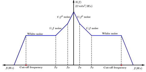
ac-celerometer, °∕s for a gyrometer… ). Figure 1.6 presents an overview of a two-sided PSD graph, which is frequently plotted in a log-log form (Units2_{/Hz versus Hz). As mentioned before, this}

graph is obtained by analyzing an ensemble of measurements given by a sensor over a long period of time with an input equal to zero (i.e. a null input signal). Through this plot it is possible to determine the power density of white noise (slope 0), 1∕𝑓 noise (slope -1) and 1∕𝑓2_{noise (slope}

-2). PSD graph does not contain any information about systematic errors.

Figure 1.6 – A general example of a two-sided PSD graph. This is a log-log graph with Units2_/Hz

vs Hz.

• White noise has a constant PSD that is described by [21]:

𝑆(𝑓)_𝑤𝑛= 𝑄2 (1.7)

where 𝑆(𝑓)𝑤𝑛 is the two-sided PSD of white noise in function of frequency 𝑓, and 𝑄 is

the constant related to the power of this noise. PSD is scaled in Units2_{/Hz, and for sensors,}

the square root of this value can be found in the datasheets but it is typically converted into an equivalent physical input and given for a one-sided PSD graph. For example, a noise equivalent acceleration is often given in 𝜇g/Hz1∕2 _{for an accelerometer. This value}

corresponds to 2𝑄. 𝑆(𝑓)_𝑤𝑛can be obtained from this value by dividing by 2 and then squared the result.

𝑆(𝑓)_𝑝𝑛= ( 𝐵2 2𝜋 ) 1 𝑓 (1.8)

where 𝑆(𝑓)𝑝𝑛is the two-sided PSD of 1∕𝑓 noise, and 𝐵 is the bias instability coefficient.

Often constant 𝐵 is not included into sensor data sheets. • Finally, PSD function of 1∕𝑓2_{noise is described by [21]:}

𝑆(𝑓)_𝑏𝑛= ( 𝐾 2𝜋 )2 ₁ 𝑓2 (1.9)

where 𝑆(𝑓)_𝑏𝑛is the two-sided PSD of 1∕𝑓2_{noise, and 𝐾 is the random walk coefficient. As}

a note, parameter 𝐾 is usually not included in sensor datasheets.

Consider a sensor with a null input signal (i.e., equal to zero). Then, the PSD from measure-ments of this sensor will be the PSD of its noise. Taking equations 1.7, 1.8 and 1.9, the PSD of the noise present in a sensor can be defined as:

𝑆(𝑓) = 𝑆(𝑓)_𝑤𝑛+ 𝑆(𝑓)_𝑝𝑛+ 𝑆(𝑓)_𝑏𝑛 (1.10)

Note that effects produced by lower frequency noises are neglected. Figure 1.6 shows how each noise is dominant at certain frequencies. For example, white noise is dominant from 𝑓𝑄 to

the cut-off frequency given by the anti-aliasing filter at the output of the sensor. 1∕𝑓 noise is dominant between 𝑓_𝐵 (the corner frequency with 1∕𝑓2_{noise) and 𝑓}

𝑄 (the corner frequency with

white noise). Below 𝑓𝐵1∕𝑓2noise is dominant. Above 𝑓𝑄white noise is dominant. Finally, 1∕𝑓2

noise is dominant below 𝑓𝐵.

It is important to observe, that equations (1.7), (1.8) and (1.9) are related with a two-sided PSD representation. In an one-sided PSD graph, those powers are doubled [25].

1.4.1 Quantifying stochastic errors by means of a PSD graph

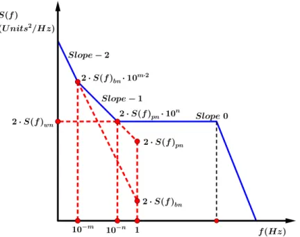
To exemplify this process of extracting parameters from a PSD graph, figure 1.7 will be used. Here, it is assumed that horizontal axis 𝑓 is given in Hz, and vertical axis 𝑆(𝑓) is given in Units2_Hz−1_.

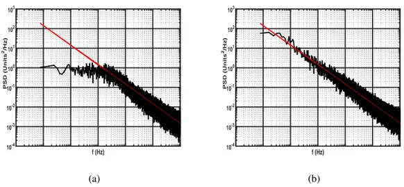
It is important to note however, that figure 1.7 shows now a one-sided PSD graph, which means that the values read directly from this graph will be multiply by a factor of two. Quantification of white, 1∕𝑓 and 1∕𝑓2_{noises from this graph is described below.}

• As equation (1.15) shows, power spectral density of white noise 𝑆(𝑓)_𝑤𝑛presents a constant behavior for all 𝑓 in a bandwidth. The magnitude of this noise is measured in Units2_∕Hzby

reading the flat region of the graph and then (because Figure 1.7 is a one-sided representation) divided by 2. Parameter 𝑄 can also be obtained by reading the flat region of the graph, divided by two and then computing the square root of it. Parameter 𝑄 is given in Units⋅√Hz. • Power spectral density of 1∕𝑓 noise 𝑆(𝑓)𝑝𝑛presents a slope -1 behavior in a log-log graph.

The magnitude of this noise is measured in Units2_{∕Hzby reading the value of this slope at}

𝑓 = 1Hz and then divided by two (due to Figure 1.7 is a one-sided representation). If the

graph does not present a slope -1 at 𝑓 =1Hz, then the 1∕𝑓 noise behavior is extrapolated with a slope -1, or read at 𝑓 = 10−𝑛_{Hz(where 𝑛 ∈ ℤ) and then divide it by 10}𝑛_{(as shown}