HAL Id: hal-00318818
https://hal.archives-ouvertes.fr/hal-00318818
Submitted on 1 Jan 2001
HAL is a multi-disciplinary open access
archive for the deposit and dissemination of
sci-entific research documents, whether they are
pub-lished or not. The documents may come from
teaching and research institutions in France or
abroad, or from public or private research centers.
L’archive ouverte pluridisciplinaire HAL, est
destinée au dépôt et à la diffusion de documents
scientifiques de niveau recherche, publiés ou non,
émanant des établissements d’enseignement et de
recherche français ou étrangers, des laboratoires
publics ou privés.
transport, mesoscale photochemistry, and
boundary-layer processes on the lower tropospheric
ozone dynamics in early spring
S. Brönnimann, F. C. Siegrist, W. Eugster, R. Cattin, C. Sidle, M. M.
Hirschberg, D. Schneiter, S. Perego, H. Wanner
To cite this version:
S. Brönnimann, F. C. Siegrist, W. Eugster, R. Cattin, C. Sidle, et al.. Two case studies on the
inter-action of large-scale transport, mesoscale photochemistry, and boundary-layer processes on the lower
tropospheric ozone dynamics in early spring. Annales Geophysicae, European Geosciences Union,
2001, 19 (4), pp.469-486. �hal-00318818�
Annales
Geophysicae
Two case studies on the interaction of large-scale transport,
mesoscale photochemistry, and boundary-layer processes on the
lower tropospheric ozone dynamics in early spring
S. Br¨onnimann1,*, F. C. Siegrist1, W. Eugster1, R. Cattin1, C. Sidle1, M. M. Hirschberg2, D. Schneiter3, S. Perego4, and H. Wanner1
1Institute of Geography, University of Bern, Hallerstr. 12, CH-3012 Bern, Switzerland
2Lehrstuhl f¨ur Bioklimatologie und Immissionsforschung, TU M¨unchen, Am Hochanger 13, D-85354
Freising-Weihenstephan, Germany
3MeteoSwiss, Station a´erologique, Les Invuardes, CH-1530 Payerne, Switzerland 4IBM Switzerland, Altstetterstrasse 124, CH-8010 Z¨urich, Switzerland
*present affiliation: Lunar and Planetary Laboratory, University of Arizona, 1629 E. University Blvd., Tucson,
AR 85721–0092, USA
Received: 23 October 2000 – Revised: 7 March 2001 – Accepted: 15 March 2001
Abstract. The vertical distribution of ozone in the lower
troposphere over the Swiss Plateau is investigated in detail for two episodes in early spring (February 1998 and March 1999). Profile measurements of boundary-layer ozone per-formed during two field campaigns with a tethered balloon sounding system and a kite are investigated using regular aerological and ozone soundings from a nearby site, mea-surements from monitoring stations at various altitudes, back-ward trajectories, and synoptic analyses of meteorological fields. Additionally, the effect of in situ photochemistry was estimated for one of the episodes employing the Metphomod Eulerian photochemical model. Although the meteorologi-cal situations were completely different, both cases had el-evated layers with high ozone concentrations, which is not untypical for late winter and early spring. In the February episode, the highest ozone concentrations of 55 to 60 ppb, which were found at around 1100 m asl, were partly advected from Southern France, but a considerable contribution of in
situ photochemistry is also predicted by the model. Below
that elevation, the local chemical sinks and surface depo-sition probably overcompensated chemical production, and the vertical ozone distribution was governed by boundary-layer dynamics. In the March episode, the results suggest that ozone-rich air parcels, probably of stratospheric or upper tropospheric origin, were advected aloft the boundary layer on the Swiss Plateau.
Key words. Atmospheric composition and structure
(pollu-tion – urban and regional; troposphere – composi(pollu-tion and
Correspondence to: S. Br¨onnimann (broenn@giub.unibe.ch)
chemistry) – Meteorology and atmospheric dynamics (meso-scale meteorology)
1 Introduction
In recent years a number of studies have reported unusually high near-surface ozone concentrations in many regions of the northern mid-latitudes already in early spring (e.g. Waka-matsu et al., 1998; Br¨onnimann, 1999). Although the mag-nitude of these peaks is smaller than that of typical summer episodes, they may, nevertheless, be important for air quality issues, since they occur at a time of year where some recep-tors are more vulnerable (e.g. during leafing of trees). In Switzerland, the 1-hour air quality standard for ozone (120 µg m−3) is sometimes already exceeded in February, and peaks >100 ppb have been observed in March (Br¨onnimann, 1999). The causes for these episodes are not clear.
A lot has been learned about lower tropospheric ozone from studying summer episodes. Ozone is created in the atmosphere as a by-product of oxidation processes and can persist and accumulate or be transported during special me-teorological conditions. An insight into the complex inter-play between chemical and transport processes has emerged as a result of many international programmes and projects that have been conducted in the last decade (see Solomon et al., 2000). One finding is that summertime ozone accumu-lation is a multi-scale phenomenon (Schere and Hidy, 2000; Wotawa and Kromp-Kolb, 2000).
photo-oxidat-ion is much slower and hence, the chemical lifetimes of many substances are longer (Parrish et al., 1999; Monks, 2000). In addition, the dynamics of the lower troposphere and espe-cially the planetary boundary layer is different than in sum-mer. The vivid discussion on the origin of the spring ozone maximum in the annual cycle at certain locations (Monks, 2000), to which early ozone episodes contribute, also makes clear that our understanding of the processes governing the ozone variability in the lower troposphere is still limited. For example, relatively little is known about the photochemistry in late winter and spring (Parrish et al., 1999).
In this study, the variability of vertical ozone profiles in late winter and spring is discussed in detail for two contrast-ing episodes on the Swiss Plateau in February 1998 and in March 1999. Both episodes showed high ozone concentra-tions at some altitude above ground, yet both were com-pletely different from a meteorological point of view. The goal of our study was to explain the following: why have high concentrations of ozone been observed at the correspond-ing altitudes, where has this ozone originally been formed, why has this not been observed at other altitudes, and which processes on which spatial scales were involved in shaping the profiles? Our study is based on tethersonde measure-ments from field campaigns embedded in an analysis of rou-tine data. Further investigations are performed with the help of trajectory models and with a photochemical model.
2 An overview of relevant processes
Different processes are relevant for the vertical ozone dis-tribution in the lower atmosphere at northern mid-latitudes. The large-scale processes include stratospheric intrusions (e.g. Schuepbach et al., 1999; Stohl and Trickl, 1999), large-scale transport (Jacob et al., 1999) and “slow chemistry” based on the oxidation of CO and CH4(Crutzen et al., 1999). Due
to mixing, dispersion, and chemical processing, air masses loose their original properties during the course of the trans-port, so that large-scale transport is not thought to be more than a “preconditioner” for high-ozone episodes. Yet, coher-ent large-scale transport of ozone from the boundary layer, or from stratospheric intrusions over distances of several thou-sand kilometres has been reported by Stohl and Trickl (1999). Photochemical ozone formation on the regional scale and mesoscale transport are usually more important in determin-ing high ozone episodes (e.g. Ryan et al., 1998). Chemical formation is most efficient close to emission sources, with more reactive hydrocarbons being oxidised and the ample supply of NOx as catalysts (e.g. Jenkin and Clemitshaw,
2000). In addition to anthropogenic emissions, the regional biogenic emissions can contribute significantly in summer (Staffelbach and Neftel, 1997). Local to regional modifica-tions of the large-scale flow can also be important. In a com-plex topography this can lead to the creation of elevated lay-ers with enhanced ozone concentration, as studied, for exam-ple, in the Los Angeles basin (McElroy and Smith, 1993) and in the Lower Fraser Valley (McKendry et al., 1997; see also
the review by McKendry and Lundgren, 2000). Low-Level Jets (LLJ) can promote downward transport of ozone from an elevated layer to the surface (Corsmeier et al., 1997; Ryan et al., 1998; see also Hidy, 2000). The effect of local flow mod-ification on pollutant transport in complex terrain has been studied intensively within the TRACT project (Fiedler and Borrell, 2000; see also the special issue of Atmospheric En-vironment, Vol. 32, No. 7, 1998) and also within the POL-LUMET project (see next section). For the Alps, the influ-ence of typical mountain effects, such as Foehn and valley winds on the transport of ozone and precursors, was recog-nised some time ago (Whiteman, 2000). These processes were studied in the VOTALP project (see special issue of At-mospheric Environment, Vol. 34, No. 9, 2000, especially the contributions of Furger et al., Pr´evˆot et al., Seibert et al., and Wotawa et al.). Furthermore, Schuepbach et al. (1999) demonstrated the possible importance of gravity wave break-ing in the lee of the Alps for ozone transport from the free troposphere to the surface.
The local scale has an influence on turbulent mixing and boundary-layer processes as well as on surface deposition. In typical summer episodes, the mixing of the boundary layer in the morning efficiently disperses the pollutants emitted at the surface. Ozone formation takes place in the whole of the boundary layer, whereas the sink is mainly at the surface (de-position, chemical sinks, titration). This leads to the typical belly shaped vertical ozone profiles. During the night, ozone is efficiently depleted in the stable nocturnal surface layer, but to a much lesser extent in the so-called “residual layer”, where some of the ozone is stored (Neu et al., 1994; for a cli-matological framework see Aneja et al., 2000). The mixing on the next morning leads to an increase in ozone concentra-tion at the surface and to a decrease in the residual layer.
This is the inventory of processes with which one has to explain the variability of vertical ozone distribution in the lower troposphere in spring.
3 The study area
The Swiss Plateau is located between two mountain ranges (Fig. 1), the Jura mountains in the Northwest and the Alps in the Southeast. The topography displayed in Fig. 1 is the one used in the “Swiss Model”, which was, among others, employed for trajectory calculation. The Swiss Plateau is a densely populated region comprising a large part of the eco-nomic activity of Switzerland. The location of the tether-soundings, Kerzersmoos (435 m asl), is a rural site in the central part of the Swiss Plateau (“Seeland”), a region with a rather flat topography and intensive agriculture (Eugster et al., 1998); for a detailed description, see Siegrist (in press). Important monitoring sites are located at Payerne (496 m asl, aerological soundings, meteorology and air pollution moni-toring) on the Swiss Plateau, and Chaumont (1140 m asl, air pollution monitoring) on the first ridge of the Jura mountains. The flow on the Swiss Plateau is channelled between the two mountain ranges, so that the winds are either from the
Southwest or from the Northeast (denoted “Bise”, Wanner and Furger, 1990). This channelling effect reaches up to around 3500 m asl. A jet is sometimes observed in the wind profile at Payerne at about 1000 m asl (Furger, 1990). At the surface, the Swiss Plateau receives cold air by drainage flows from the Alps as well as from the Jura mountains. Cold air layers can be very persistent in winter. In summer, the ex-change with the alpine valleys is efficient and can amount to one-third of the volume of the boundary layer over the Swiss Plateau every day (Neininger and Dommen, 1996).
High ozone values occur on the Swiss Plateau each sum-mer and have been investigated in various studies, espe-cially in the POLLUMET project (Neininger and Dommen, 1996; Wanner et al., 1993; Pr´evˆot, 1994; Dommen et al., 1995; 1999; see also the special issue of Meteorologische Zeitschrift, N. F. 2, August 1993). A statistical analysis of aerological soundings from Payerne showed that trans-port distances during summer smog episodes are normally only around 50 to 100 km/day at the surface and 150 to 200 km/day at 1000 m asl, with somewhat higher values for the residual layer during the night (Jeannet et al., 1996). Hence, a large fraction (around 20 ppb) of the ozone peaks observed on the Swiss Plateau during summer episodes must be pro-duced in situ over the Swiss Plateau (Neininger and Dom-men, 1996), as was also supported by experimental (K¨unzle and Neu, 1994) and model studies (Dommen et al., 1995; Perego, 1999). It was shown that ozone formation in summer on the rural Swiss Plateau is mainly NOxlimited (Dommen
et al., 1995). Plumes of cities, especially Zurich, were also identified to influence ozone on the Swiss Plateau (Dommen et al., 1999). The monitoring of time series revealed that ozone episodes frequently occur already in early spring at some elevation over the Swiss Plateau (Br¨onnimann, 1999).
The Seeland was a core region within the POLLUMET project with detailed chemical measurements on Mount Vully and tethered balloon soundings. With these data, the question of NOx or VOC limitation was addressed and
typ-ical concentration ranges for many trace species were deter-mined. Trajectory analyses suggested that the origin of air masses is important in this region, especially when air masses have passed over the urban region of Lyon (Pr´evˆot, 1994).
The Swiss Plateau is a suitable area for detailed case stud-ies. It can be considered a well investigated region with re-spect to air chemistry in a topographical setting of interme-diate complexity. The area under investigation is usually re-ferred to as rural, although the Swiss Plateau, as a whole, is relatively densely populated.
4 Data and Methods
This study makes use of many data sets and involves the ap-plication of several computer models. This section provides the relevant references for data sets, data quality, models, previous model applications, and validations.
The tethered balloon system from Atmospheric Instrumen-tation Research, Inc. (A. I. R., Boulder, CO, USA) consists
Fig. 1. Map of the study area with the locations of all
measure-ment sites. The rectangle indicates the domain considered for pho-tochemical modeling. Shaded areas give the topography from the Swiss Model (SM). Contour lines are drawn at 500, 750, 1000, 1500, 2000 and 3000 m asl.
of a 57 m3helium-filled balloon on a 1800 m tether, a KI based ozone sonde OZ-3A-T (Baumbach et al., 1993), and a meteorological TS-5A-SEN (A. I. R.) sonde for tempera-ture, relative humidity, pressure, wind speed and direction. Ozone soundings usually show somewhat higher values dur-ing descent than durdur-ing ascent, which could be due to time lags and to decreasing voltage of the battery. Ascents are generally considered to be more reliable than descents.
Aerological soundings performed at Payerne include wind profiles every 6 hours, meteorological soundings every 12 hours (SRS-400 sonde, Richner and von H¨unerbein, 1999) and ozone soundings three times per week (BM sonde, Hoeg-ger et al., 1999; St¨ubi et al., 1999; 2000). Ozone sonde mea-surements in the lower troposphere should be considered as less accurate than surface measurements, but the shape of the profiles should be reliable.
Station measurements of chemical and meteorological pa-rameters for Payerne, L¨ageren, Chaumont, Rigi, T¨anikon, Davos, and Jungfraujoch were taken from the Swiss air qual-ity monitoring network NABEL (EMPA, 1994). Meteorolog-ical data from Payerne, T¨anikon, and Jungfraujoch were pro-vided by MeteoSwiss. CO data from Jungfraujoch are from EMPA (Swiss Federal Laboratories for Materials Testing and Research, D¨ubendorf). In addition, station measurements of ozone and humidity from Zugspitze were provided by IFU (Fraunhofer-Institut f¨ur Atmosph¨arische Umweltforschung, Garmisch-Partenkirchen).
Three-dimensional backward trajectories were calculated with three models and different meteorological fields rep-resenting different scales. We used the HYSPLIT-4 model from NOAA (Draxler and Hess, 1997, 1998) in conjunc-tion with FNL archived meteorological data (Stunder, 1997).
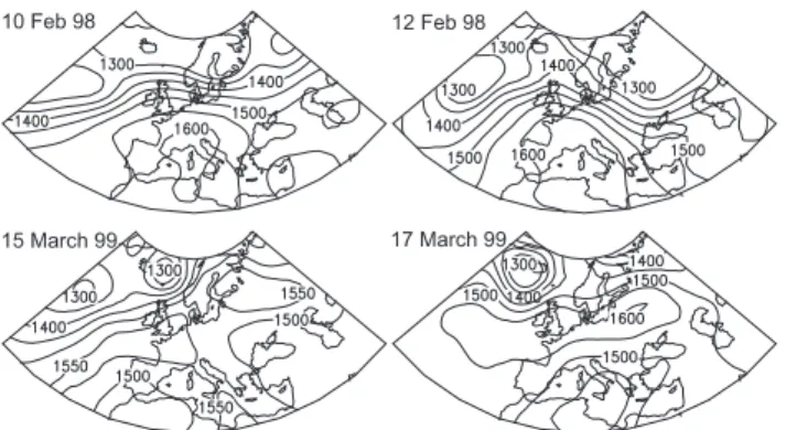
Fig. 2. 850 hPa geopotential height field over Europe on 10 and
12 February 1998 (top) and 15 and 17 March 1999 (bottom), at 12 UTC. Contour lines are in units of geopotential meters.
The FLEXTRA model Version 1 (Stohl et al., 1995) was used together with wind fields from the ECMWF T213-L31 data set (ECMWF, 1994), interpolated to a 0.5◦×0.5◦grid with 3-hourly resolution. Finally, we also used backward trajectories calculated with the DWD trajectory model TRA-JEK (Fay et al., 1994) based on the meteorological HRM/SM forecast model (High resolution model/Swiss Model, Schu-biger and DeMorsier, 1992), which has a resolution of 14 × 14 km2and an appropriate orography (Fig. 1).
Numerical modelling was performed with the Metphomod model (Perego, 1999), a three-dimensional Eulerian photo-chemical model for the simulation of summer smog. The model includes a dynamical meteorological model, a soil module, and a solver for gas phase chemistry. Here we use the updated version 2.1, which includes a two-stream radi-ation module (based on the TUV model, Madronich et al., 1997) for calculating photolysis rates. More information about this model version can be found on the website indi-cated at the end of this article. Synoptic and meteorological analysis was performed with NCEP/NCAR reanalysis data (Kalnay et al., 1996) on a 2.5◦×2.5◦ grid. Additionally,
Meteosat water vapour images (provided by EUMETSAT) and total ozone data (TOMS version 7) from Earth Probe (McPeters et al., 1996) were used.
5 Results
In this section observational data and model calculations for both case studies are presented in a descriptive manner, start-ing with the tethered balloon and kite soundstart-ings at Kerz-ersmoos and ending with a presentation of trajectories and large-scale flow conditions. A discussion for each of the case studies is given in Sect. 6.
5.1 Tethered balloon and kite soundings 5.1.1 February 1998
The field campaign in February 1998 (Cattin, 1998) took place during a late winter high pressure episode. Air
tem-peratures were relatively high, i.e. around 12◦C in the
af-ternoon, but the soil was still around 0 ◦C. The winds at
the surface were weak during most of the campaign, mainly from the Southwest. Figure 2 shows the geopotential height at the 850 hPa level on 10 and 12 February. Switzerland was slightly north of the centre of a high-pressure system, which moved slowly to the West during the episode. The campaign began on 10 February, in the evening, and lasted until the early afternoon of 12 February. A total of 25 sound-ings were performed. Since the wind speed was relatively high at around 900 m above ground, the balloon could not always penetrate into the layer aloft.
The data are displayed in Fig. 3a. The time-height cross sections of virtual potential temperature, θv, show a fairly
stable atmosphere. Some mixing is indicated for the after-noons of 11 and 12 February, but the mixing layer, derived from θv, remained shallow, around 300 to 400 m deep. The
water vapour mixing ratio, r, was relatively high, up to around 500 m above ground, but decreased aloft to rather low values. The boundary between the moist and the dry air was not the same as the estimated mixing height.
The amplitude of the diurnal ozone cycle was large at the surface. Ozone concentrations were practically zero at night, when a stable surface layer is clearly visible in the time-height cross section of θv. During the day, ozone
concen-trations at the surface increased to around 35 ppb. At about 1000 m asl, ozone concentrations, at all times, were consid-erably higher than at the surface. They were around 40 to 50 ppb and reached a maximum of 55 ppb, which is high for this time of the year, on the afternoon of 11 February at 900 m asl.
5.1.2 March 1999
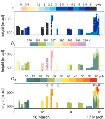
The second campaign in March 1999 (Cattin, 1999) started at the end of a short and moderate early spring ozone episode. Compared to the February campaign, the pressure distribu-tion was rather flat in the beginning. During the following days, a high pressure ridge formed over Germany (Fig. 2), and Switzerland was in an easterly flow. Wind speeds at the Kerzersmoos site began to increase during 16 March, mak-ing balloon soundmak-ings impossible. A kite was used instead of the tethered balloon during the day (marked with “K” in Fig. 3b), reaching altitudes of up to 1140 m asl. The winds further increased during the morning of 17 March. Three soundings were performed with the kite during that morning, with wind speeds reaching 20 m/s, until a wind gust destroyed the kite and the sonde. The time-height cross sections differ signifi-cantly from the ones of the February campaign; the soil was warmer and the boundary layer was well mixed. θvincreased
and decreased synchronously at all heights but, in total, ex-perienced a cooling through the episode. The humidity was high, up to a height of around 1000 m asl. The nocturnal profiles show that the atmosphere was slightly stratified (i.e. stable) during the night from 15 to 16 March, but probably mixed during the night from 16 to 17 March.
Fig. 3a. Time-height cross sections of virtual potential temperature,
water vapour mixing ratio, and ozone concentrations as measured with tethered balloon during the February 1998 campaign. Every ascent or descent was attributed to a fixed half-hour interval.
on 16 March. The most interesting feature during the cam-paign were the high-ozone levels above 1000 m asl in the morning on 17 March. Winds were very strong throughout the sounded profile. There was a sharp increase of ozone, from about 30 ppb at 750 m asl, to 60 ppb at 1100 m asl, and a simultaneous decrease of the water vapour mixing ratio, r, from 3 g/kg to values below 1 g/kg. The profiles of θvdisplay
a clear inversion at around 1000 m asl.
The data from the field campaigns reveal two contrast-ing episodes. In both cases, high ozone concentrations were found at some altitude above the surface. In the February 1998 campaign, ozone was not related to humidity and it remains unclear as to what extent different air masses were involved. In contrast, the March 1999 campaign clearly re-veals the influence of several distinctly different air masses and, therefore, points to an important influence of transport processes.
Fig. 3b. Time-height cross sections of virtual potential temperature,
water vapour mixing ratio, and ozone concentrations measured with tethered balloon or kite (marked with K) during the March 1999 campaign.
5.2 Aerological soundings and station data
The data from the field campaigns give a detailed, yet incom-plete picture of what was happening in the lower atmosphere over the Swiss Plateau during these days. With a coarser tem-poral resolution and on a somewhat larger scale, they can be complemented with aerological soundings from Payerne and suitable station data.
5.2.1 February 1998
Time-height cross sections based on Payerne soundings, up to a height of 3500 m asl, are displayed in Fig. 4 for the two case studies. Before the campaign, the general wind direc-tion was from the Northeast. Then the winds changed to the Southwest for the period of the campaign. The wind speed cross section shows a jet-like behaviour during 11 February, just above the altitude of the adjacent Jura mountains. At the end of the campaign, the wind direction turned back to the Northeast.
The time-height cross section of θv in the February 1998
case reveals a relatively stable atmosphere. According to the difference in θvwhich was measured at screen-height (2 m),
mixing remained shallow, at least around 13 CET. The at-mosphere was relatively humid. The drier layer observed in Fig. 3a is also visible in the Payerne soundings. Temper-atures were rather warm for the time of the year, although such warm “early spring” episodes are not uncommon for
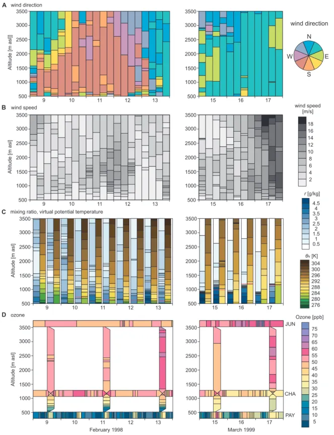
Fig. 4. Time-height cross sections of (a) wind direction, (b) wind speed, (c) water vapour mixing ratio (left bars) and virtual potential
temperature (right bars) and (d) ozone concentrations. Left panels: February 1998 campaign, right panels: March 1999 campaign. The plots show measured data from aerological soundings from Payerne which were supplemented with hourly averaged station measurements of ozone concentration. No interpolation was done. Data were plotted as raw data and every measurement point was attributed to half of the layers above and below the measurement altitudes except for wind (layer below). Note that wind soundings were performed every 6 hours (00, 06, 12, 18 UTC), full meteorological soundings every 12 hours (00, 12 UTC) and ozone soundings every two days (12 UTC). The red solid lines in panels (c) give the estimated mixing height.
Switzerland in February. A warming took place during the course of the episode.
Since the time resolution of ozone soundings was very coarse (2 days) when compared to the field campaigns, time-height cross sections of ozone were complemented with sta-tion measurements (horizontal bars in Fig. 4) from Payerne, Chaumont, and Jungfraujoch (Fig. 1). Ozone concentrations at the surface and in the boundary layer, at noon, were very low, 30 to 35 ppb at most, with a distinct diurnal cycle. In the evening, they rapidly sank to values below 5 ppb, indicating a strong local sink. Concentrations at Chaumont were higher than at Payerne at all times by at least 20 ppb. Combined with the strong gradient apparent in the Payerne ozone pro-files at noon, this again indicates incomplete mixing. Ozone concentrations at Chaumont were between 45 and 60 ppb, with a diurnal cycle, and were higher at almost all times than at the high-alpine site Jungfraujoch.
5.2.2 March 1999
During the March 1999 campaign, winds were persistently from the Northeast (“Bise”). Wind speeds were moderate at the beginning, again with some jet-like features, then in-creased throughout the lower troposphere and reached 20 m/s in the morning of 17 March.
Time-height cross sections of θvand r in March 1999
re-veal a well developed mixing layer. The mixing height, as estimated from the difference between θv and θv at the
sur-face, corresponds well with the sharp gradient in the mixing ratio profiles. The atmosphere above was very dry, confirm-ing that there must have been two different air masses.
In the time-height cross section of ozone for March 1999, the end of a short ozone episode is visible at Payerne and Chaumont, with peaks reaching 60 ppb (the maximum at Chaumont on 14 March was 64 ppb). Ozone concentra-tions in Payerne showed a clear diurnal cycle. Nocturnal concentrations were almost zero during the first two nights (14/15 and 15/16 March), but somewhat higher during the night from 16 to 17 March. Daily peaks decreased from 56 ppb on 15 March to 30 ppb on 17 March. The small differ-ence in ozone concentrations between Chaumont and Pay-erne again points to good mixing during the day; this is also indicated by the Payerne ozone profiles. Ozone concentra-tions at Chaumont showed a clear diurnal cycle only on the first day (15 March), then the diurnal cycle became less clear and was absent on 17 March and concentrations strongly de-creased. Payerne ozone soundings show an increase of ozone from 15 to 17 March in the free troposphere. On 17 March, two local maxima appeared at heights around 1700 and 2700 m asl.
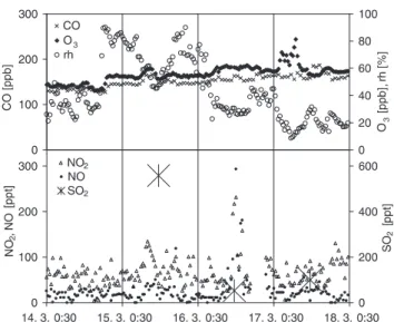
At Jungfraujoch, ozone concentrations were clearly higher than at Chaumont, especially from 16 March onward. Most remarkably, two short peaks of 72 and 81 ppb (half hour val-ues) were observed during the night from 16 to 17 March. These sharp peaks were preceded by a smaller, smoother in-crease during 16 March. Figure 5 shows Jungfraujoch sta-tion measurements of NO, NO2, CO, SO2, relative
humid-Fig. 5. Measurements of ozone, NO, NOx, SO2, CO, and relative
humidity at Jungfraujoch from 14 to 17 March 1999. Note that SO2
data are daily average values.
ity, and ozone from 14 to 17 March. Different changes in air mass can be addressed within this time span. The high-ozone event during the morning of 17 March was accompanied by a sharp drop in humidity, to values below 10%, with low SO2
concentrations and low NOx levels of around 60 ppt. Little
changes, however, were observed in CO concentrations. The analysis of aerological soundings reveals additional features in both episodes. In February 1998, the high ozone levels at around 1200 m asl and the occurrence of a jet in the wind profile at the same height direct our focus towards this altitude. In March 1999, the data imply the picture of many changes, a sequence of different air masses and sharp spa-tial gradients of air mass properties. Ozone concentrations reached 81 ppb at Jungfraujoch. The spiky character of the ozone peak and the low levels of humidity, NOx, and SO2
point to a stratospheric intrusion as a possible source. This hypothesis will be further discussed in Sect. 5.4.
5.3 Mesoscale photochemical modelling
The measured ozone profiles during the February 1998 episode bear many features in common with typical summer-time ozone profiles, such as the diurnal cycles at all levels and the ozone maximum at some altitudes above the ground. Photochemistry is, therefore, considered as a possible driv-ing factor. On the other hand, solar radiation is very low in mid-February and hence, photochemistry is only expected to proceed very slowly. The question of whether ozone can be formed photochemically in a sufficient amount, so early in the season as to explain these features, will be tackled in this section with the aid of the photochemical Metphomod model (Perego, 1999).
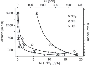
Fig. 6. Measurements of NO, NO2 and CO at different sites on
9 February, 11 to 13 UTC, and initial values prescribed to the 18 levels of Metphomod by fitting a power law to the measured con-centrations (the value in the lowest model layer was replaced with the value from the second lowest layer).
5.3.1 Setup of the model experiment
The square in Fig. 1 gives the model domain. It comprises a large part of the Swiss Plateau as well as the pre-alpine foothills and the first chain of the Alps. The model used a horizontal grid of 100 × 45 cells at a resolution of 2 × 2 km2 with 18 vertical levels (Cartesian, see Fig. 6). A fixed time step of 10 s for meteorology and a variable one (1 to 120 s) for chemistry were chosen. The chemical RACM mech-anism (Stockwell et al., 1997) was used. Quantum yields and absorption cross sections were taken from the RACM (Stockwell et al., 1997 and references therein; Frank Kirch-ner, personal communication, 2000), except for R1 to R3, which were taken from the TUV model (Madronich et al., 1997). The quantum yields for ozone photolysis were taken from Shetter et al. (1996). Total ozone was set to 400 DU, and radiation was calculated for every grid-point for every 120 s.
The model had been developed for summer situations and was first used for the Swiss Plateau. For input and border data, we could partly rely on these data, which are described in Perego (1999). They include emissions from the detailed TRACT inventory (Kunz et al., 1995) as well as surface data. The soil properties had to be adapted to winter conditions. Soils were assumed to be water saturated in the Swiss Plateau and partially or fully snow covered at higher altitudes, de-pending on vegetation type and exposition. Since the model does not explicitly include snow layers, the effect of snow was achieved by adjusting the soil heat diffusivity and heat capacity, as well as the albedo and the fraction of plant cover. The full input data set can be downloaded, together with the original summer input data and the model itself, from the website indicated at the end of this article. In the emission inventory, we scaled NO and NO2emissions with a factor of
1.2 (accounting for domestic heating), and α-pinene and Iso-prene emissions with a factor of 0.2 (less biological activity). We did not change the aggregation factors for the RACM classes. The model was initialised on 9 February, 13 CET with ozone and meteorology from the Payerne sounding. For other substances we used station data from different altitudes from 12 to 14 CET (average). Distinct concentration min-ima were found for almost all substances and sites during this time, which points to some degree of mixing and, therefore, a better representativity of the surface measurements for a grid cell. For NO and NO2, we used data from Payerne, T¨anikon,
L¨ageren, Rigi, Chaumont, Davos, and Jungfraujoch (Fig. 1); CO was available from T¨anikon, Chaumont, and Jungfrau-joch. A power law fitted to the station altitude provided the initialisation profiles with the exception of the surface layer, for which we used the same value as for the second layer (Fig. 6). CH4 was set to 1700 ppb and PAN to 0.18 ppb,
according to February measurements (Wunderli and Gehrig, 1991). For VOCs, data from T¨anikon, a rural site on the Swiss Plateau, were aggregated into RACM classes follow-ing Stockwell et al. (1997) and references therein, usfollow-ing the same aggregation factors. Vertical profiles were obtained by scaling the fitted profile for NO (as a representative of short-lived species) to match the observations for ETH, ETE, HC3, HC5, HC8, OLT, TOL, and XYL in the second model layer (location of T¨anikon).
The model was forced towards fixed values at the borders (border type “sponge”). For meteorological parameters and ozone, these values were taken from the soundings at Pay-erne at the main inflow border and were linearly interpolated with time. The model top (at 3450 m asl) was constrained with the geostrophic wind from the Payerne soundings. The initial data for CH4and the CO profile were also used at the
borders; all other substances were set to the average of the corresponding model level at the preceding time step.
The net chemical production of ozone was calculated with two approaches. Following an “Eulerian” framework, all concentration changes in a cell that occur due to chemical reactions (not due to mixing, dispersion, transport, or deposi-tion) were calculated for each grid cell. This production rate includes the effect of titration and reformation of ozone from NO2. This is suitable for addressing the observed changes
in the profile over Kerzersmoos, which is influenced by titra-tion/reformation. It can also be used for budget calculations when integrated over the entire model and summed up over the entire time span.
In a “Pseudo-Lagrangian” framework we introduced a chemically inert tracer that was initialised to the current ozone field at a chosen time and then transported and de-posited. The border data and deposition were the same as for ozone. With the field of the difference between the tracer and ozone, and with an additional tracer accounting for the residence time in the model, we could calculate an approximate net ozone production for an air parcel over short time periods. This production rate is not influenced by titra-tion/reformation, as long as it occurs within the considered time span. The model was run for 100 hours until 13
Febru-Fig. 7. Observed (thick lines) and modelled (thin lines) time series of NO, NO2and ozone at eight sites from 9 February, 12 UTC to 13
February, 12 UTC. For L¨ageren, which is on a 45 m tower on a steep slope, the corresponding grid cell was too low, therefore, we used a point more to the east at correct elevation.
ary, 16 UTC (17 CET). 5.3.2 Model validation
We validated the model results by comparing station mea-surements of NO, NO2, and O3from several sites with
mod-elled values for the corresponding grid cells (Fig. 7). This gives a useful indication whether the model captures the main characteristics of the spatio-temporal concentration variabil-ity. Note, however, that the model gridpoints represent grid cells of 2 × 2 km2with a height of 50 m or more, whereas the measurements very often are only locally representative. With respect to ozone, the agreement between model and measurement is very good for Rigi and reasonably good for L¨ageren, T¨anikon, and Kerzersmoos. The deviation at Chau-mont (8 cells downwind of the border) is due to the bor-der values which are too low. The nocturnal differences at L¨ageren, T¨anikon, and Kerzersmoos are due to stronger sur-face influences in the measurements (2 to 4 m above ground), as compared to the grid cell averages. This is probably also the main cause for the deviations found at the polluted sites, where the extremely high level of observed NO concentra-tions (up to 350 ppb) are not reproduced by the model. NO2
is well predicted at all sites. The decrease of NO2 and
in-crease of ozone at all polluted sites on the evening of 11 February is produced by a jet-like wind gust in the model that hits the surface layer and leads to an exchange with the upper layers. This jet existed (Fig. 4), but in reality did not reach the surface. All together, it can be said that the model shows good agreement with station data and gives realistic
results even after four days of simulation.
Figure 8 shows time-height cross sections of specific hu-midity, ozone, NO2, and the ozone production rate for the
location of Kerzersmoos. The humidity profile shows the observed dry air layer between 1400 and 1700 m asl, and distinct humidity maxima close to the surface in the early afternoon. As in the measurements (Fig. 3a), a tongue of high ozone concentrations reaches down close to the surface during the afternoon of 11 February and less pronounced on 12 February. With respect to ozone, humidity and temper-ature (not shown), the agreement between the model results and the Kerzersmoos soundings is very good. NO2exhibits
rather high values in the boundary layer, around 5 ppb or more. The diurnal cycle shows a morning peak that influ-ences the whole boundary layer.
5.3.3 Model results
The bottom panel of Fig. 8 shows the “Eulerian” net chem-ical ozone production rate. The highest values of up to 5 ppb/h are calculated after sunrise, between 8 and 9 CET at about 100 m above ground. They result from reformation of ozone titrated during the night. A second maximum appears in the early afternoon, and it is suggested that this is mainly due to photochemical production. This maximum was very pronounced on 11 February and less so on the other days. If the O3/NOzratio can also be used as a photochemical
indica-tor in winter with the thresholds given in Sillman (1995), then ozone production at Kerzersmoos during the afternoon of 11 February was VOC sensitive (O3/NOz<7), up to about 700
Fig. 8. Modelled time-height cross sections of (a) specific humidity
[g/kg], (b) ozone [ppb], (c) NO2[ppb], and (d) net chemical ozone
production rate [ppb/h] for the location of Kerzersmoos.
m asl and NOxsensitive (O3/NOz >10) above 1000 m asl.
On the other afternoons, the O3/NOzratio was intermediate
(between 7 and 10). A chemical sink reaching −2 ppb/h in the lower boundary layer and −6 ppb/h at the surface is pre-dicted for the late afternoon and after sunset. On a molecule basis, summed up over three diurnal cycles (10 Feb, 6 CET to 13 Feb, 6 CET), the surface layer over Kerzersmoos is a chemical sink that is compensated by chemical sources at an altitude of 600 m asl (i.e. within the lowest 150 m). If depo-sition is also considered, then the column over Kerzersmoos
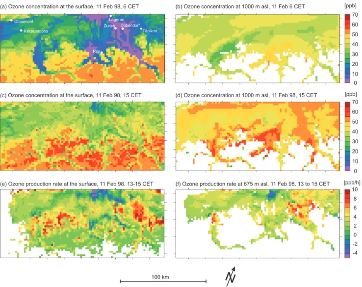
is a net sink up to 1250 m asl. Over the whole model domain, sources and sinks balance below 1750 m asl and the model is a weak source. The predicted ozone field at the surface on 11 February, 6 CET is shown in Fig. 9a. Ozone con-centrations are close to zero on the Swiss Plateau and at the bottom of alpine valleys, whereas higher concentrations are predicted at higher elevations. At 1000 m asl (Fig. 9b), there is little spatial variability; ozone concentrations are around 35 to 50 ppb. At 15 CET, surface level ozone concentrations (Fig. 9c) are around 20 to 40 ppb on the Swiss Plateau and 50 to 60 ppb at higher elevations. At 1000 m asl (Fig. 9d), concentrations between 45 and 55 ppb are predicted. Figure 9e,f show the approximate rate of ozone production during the last two hours (calculated in the “Pseudo-Lagrangian” framework) for each air parcel on 11 February, 15 CET. At the surface (Fig. 9e), air masses transported along the major traffic routes and over the cities on the Swiss Plateau are de-pleted in ozone at a rate of −2 to −4 ppb/h, whereas they are enriched at rates of 4 to 8 ppb/h in the lee of Zurich and Bern. Over large parts of the Swiss Plateau, ozone is produced at a rate of 1 to 4 ppb/h. Distinct ozone production areas are found along the south slope of the Jura mountains. The cor-responding field of the “Eulerian” production rate at noon (not shown) is mainly determined by small areas of heavy titration (up to −30 ppb/h) and reformation (+15 ppb/h) of ozone, but agrees with the 1 to 4 ppb/h obtained for rural ar-eas (also over Kerzersmoos: see Fig. 8). Interestingly, the highest production rates in the “Pseudo-Lagrangian” frame-work of 8 or 9 ppb/h are found when the plume of Zurich was advected over snow surfaces with higher albedo, where NO2
photolysis was enhanced and a new photochemical equilib-rium reached (this concerns some of the grid cells in Fig. 9e which are empty, i.e. lower than topography, in Fig. 9f). These production rates seem high, but they may be realis-tic. They reflect that temporary reversible phenomena are considered in our approach, only if they exceed the consid-ered time scale of 2 hours. Note also that the early afternoon of 11 February represents the period of the highest ozone production during these four days and, therefore, has to be considered as an upper limit. In all, according to the RACM chemical mechanism, considerable ozone production already seems possible in late winter.
5.4 Trajectory models and large-scale circulation
The analysis of tether balloon and radio sonde data suggests an important role of transport processes. This section presents an analysis of backward trajectories for both case studies, as well as a study of the synoptic context and the large-scale circulation.
5.4.1 Backward trajectories for February 1998
In February 1998, the importance of transport is indicated from the coincidence of high ozone concentrations and a jet in the vertical profile of the wind speed at about 850 hPa. Less transport is expected (due to low wind speeds) above
Fig. 9. Ozone concentration fields modelled by Metphomod for 11 February, 6 CET at the surface (a) and at 1000 m asl (b), and on 11
February 15 CET at the surface (c) and at 1000 m asl (d). Average ozone production rate in the “Pseudo-Lagrangian” framework for the last 2 hours at the surface (e) and at 675 m asl (f), for air parcels at 11 February 16 CET. The outermost two grid cells on all sides were deleted in all charts. White spots are below topography.
and below this layer. We calculated 72 hours backward tra-jectories (FLEXTRA/ECMWF), arriving at different heights over Kerzersmoos and eight surrounding points (7.17±0.25◦ E, 47.00±0.25◦N) in February 1998.
Figure 10 shows the trajectories arriving at 850 hPa. Since there was relatively little scatter within the ensembles, only the central trajectories are displayed. According to these re-sults, air masses originated from the middle troposphere over Germany/North Sea, from where they descended to 700 hPa after having crossed the Alps and further down to 850 hPa over Italy. The trajectories had a pronounced anticyclonic shape; they performed a loop west of Sardegna and flowed north-eastward towards the Swiss Plateau. Trajectories later during the episode were slower than the earlier ones, but fol-lowed almost the same path. We consider it plausible that the air masses observed at around 1000 m asl and higher over Kerzersmoos originated from the Mediterranean area
and were advected over Southern France. 5.4.2 Backward trajectories for March 1999
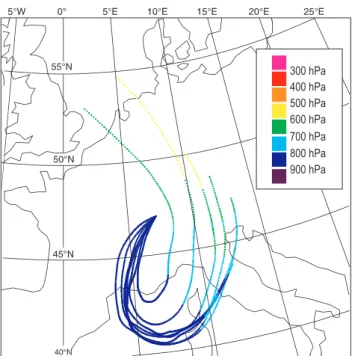
For the March episode, HYSPLIT/FNL and DWD/SM ward trajectories were used. HYSPLIT/FNL 96 hrs back-ward trajectories for different arrival heights and times for Kerzersmoos are displayed in Fig. 11. As expected from the observations, all trajectories arrive from the Northeast. On 16 March, trajectories have an anticyclonic shape and the origin is South of Greenland (for air masses arriving at 1500 m above ground), Gulf of Biscay (500 m) and Southern Ger-many (100 m), respectively. The situation is different one day later, when the lower most trajectories are still anticy-clonic, but the upper trajectories are cyclonic and originate from Russia. Ensemble trajectories (ca. 1◦lat./long. apart) for the early morning (6 UTC) of 17 March for 2500 m above ground are also displayed since their arrival time corresponds
Fig. 10. 72-h backward trajectories from FLEXTRA/ECMWF
ar-riving at Kerzersmoos at the 850 hPa level every 6 hours between 10 February 1998, 18 UTC and 12 February 1998, 12 UTC.
to the time of the high-ozone event at Jungfraujoch. All tra-jectories come from a zone of horizontal convergence at 600 hPa over Poland. However, it is very difficult to track the ori-gin of the air masses further back in time. They can oriori-ginate either from the middle troposphere south of Greenland, the Kola Peninsula or the Ural mountains, or they can originate from the boundary layer of the South-eastern Balkans.
DWD/SM 48 hrs backward trajectories for 17 March, 0 UTC are shown in Fig. 12. Trajectories arrive at differ-ent levels at Chaumont, Payerne, and Jungfraujoch and at surrounding points (ensembles of five). All the trajectories slightly descend from their origin towards the receptor site, however, not by large amounts. The lower trajectories arrive from an East-West path along the northern slope of the Alps, whereas a northern component becomes stronger with alti-tude. At 500 hPa over Payerne, air masses arrive from the North.
5.4.3 Synoptic analyses for March 1999
To further study the properties of the advected air mass, we investigated specific humidity from NCEP reanalysis data. Figure 13 displays the field of specific humidity at the 700 hPa level on 17 March, 6 UTC. We see an elongated area of very dry air with its main axis from Poland to North-ern Italy, roughly parallel to the trajectories. Values are ex-ceptionally low, down to 0.1 g/kg. This dry area compares well with the measured humidity minimum of 0.4 g/kg at Jungfraujoch. Figure 14 (top) shows station measurements from Zugspitze, which is upwind of the Swiss Plateau. It can be seen that ozone concentrations were also elevated (62
Fig. 11. 96-h backward trajectories from HYSPLIT/FNL arriving
at Kerzersmoos at different altitude on 16 March, 12 UTC (top) and on 17 March, 12 UTC (centre), and ensemble of backward trajecto-ries arriving at Kerzersmoos on 17 March, 6 UTC at 2500 m above ground (bottom). The line indicates the cross section used in Fig. 15.
ppb) on 16 March, in line with a humidity decrease, but they do not show high spikes, such as at Jungfraujoch. A second, stronger humidity decrease down to 13% was not accompa-nied by an ozone increase, but occurred at the same time as the ozone spikes at Jungfraujoch.
A number of aerological sounding stations are located close to the trajectories and the dry area shown in Fig. 13. All of them performed ozone soundings on 17 March, 12 UTC, with some already on 15 March, 12 UTC. Figure 14 shows the corresponding humidity and ozone profiles. The profiles show various ozone-rich and dry air layers. For example, a layer with humidity down to 10% with ozone concentrations of 65 ppb was observed at 2500 to 3000 m asl over Prague on 15 March. Many smaller scale features were observed in the profiles from 17 March. Ozone was very often, but not always, anticorrelated with humidity in these layers. How-ever, it is not possible to relate these layers to one another or to station measurements. Also, ozone concentrations were always lower than the ones observed at Jungfraujoch (note, again, that the accuracy of ozone sonde measurements in the lower troposphere is not very good). Low ozone concentra-tions were observed everywhere below 1100 m asl.
On a somewhat larger scale, a broad picture can be ob-tained from NCEP reanalysis data. We specified a transect parallel to the trajectories and the dry area (marked in Figs. 11, 12, and 13). Figure 15 shows a temporal (six-hourly)
Fig. 12. 48-h backward trajectories (ensembles) from DWD/SM for
17 March, 0 UTC, arriving at Chaumont, Jungfraujoch, and Payerne at various levels. The line indicates the cross section used in Fig. 15. The locations of the sounding sites used in Fig. 14 are also displayed.
series of cross sections of specific humidity along the tran-sect. The 0.25 g/kg isoline shows a southward moving and slightly descending tongue of dry air, reaching the Alps on 17 March, 6 UTC. This is again in good agreement with hu-midity at Zugspitze and Jungfraujoch. The agreement with the soundings is worse at first sight, but is reasonable if one considers the coarse resolution of NCEP data.
From the trajectories, the soundings, and the humidity cross section, it seems plausible that stratospheric or upper tropospheric air has found its way down to the Swiss Plateau. If so, where did this air come from? A glimpse at the conti-nental scale is given in Fig. 16. It shows water vapour images (5.7–7.1 µm) from METEOSAT, tropopause pressure from NCEP data, and total ozone from TOMS Version 7 data for 13, 15 and 17 March. Water vapour images show streamers of dry air, most pronounced over Southern France/Corse on 17 March, 12 UTC. They were probably related to the dry air area found in Figs. 14 and 16. Slightly east of this dark area, the tropopause is low, and total ozone reaches 480 DU. These are areas where stratosphere-troposphere exchange can oc-cur. The whole situation evolved from an upper low, north of the Black Sea. It is possible, therefore, that the ozone-rich air parcels hitting the Swiss Plateau were transported on the northern flank of this upper low towards the Alps.
Fig. 13. Specific humidity [g/kg] at the 700 hPa level from NCEP/NCAR reanalysis data for 17 March, 6 UTC. The line in-dicates the cross section used in Fig. 15.
6 Discussion
In this section, the results from both episodes are discussed and interpreted and the findings are compared to literature. The most important features for both cases are summarised in Table 1.
6.1 February 1998
The February 1998 case can be considered as a typical late winter high-pressure episode with only light winds and high temperatures for the season. Ozone concentrations reached relatively high levels at some elevation above the surface. The pronounced diurnal ozone cycle at the surface was due to a strong ozone sink at the surface (deposition and chemi-cal destruction) in connection with the changing atmospheric stability of the lowest layer, i.e. a small volume and little ex-change at night compared to a larger volume and more effi-cient exchange during the day.
In the morning, the model predicts a slight ozone increase at the surface (3 to 5 ppb) from the reformation of ozone that was titrated during the night. The observed increase of sur-face ozone during the day, however, was mainly caused by downward mixing of ozone-rich air from aloft. The model predicts only a weak source at the surface during the day, whereas deposition is a strong sink. The downward mixing, on the other hand, was limited by the atmospheric stratifica-tion and, therefore, a vertical gradient of the ozone concen-tration was always maintained.
At around 50 to 800 meters above the ground, photochem-ical ozone formation provides an ozone source, according to our model using the RACM mechanism. On 11 February, this production was especially strong. In the lowest layers it was probably limited by VOCs, in contrast to summer condi-tions. A seasonal transition from a NOxlimited
photochem-Fig. 14. Measurements of ozone concentration (thick lines) and
rel-ative humidity (thin lines) at Zugspitze from 15 to 17 March 1999 (top). The centre and lower panels show ozone and humidity pro-files for 15 March, 12 UTC, and 17 March, 12 UTC from different locations in Europe (indicated in Fig. 12). Note that the scale for relative humidity is inverted in all panels.
istry in summer to a VOC limited one in winter was also suggested by Jacob et al. (1995) for the eastern US. The pre-dicted net chemical production rates at 675 m asl in the early afternoon (Fig. 9f) are roughly 1 to 4 ppb/h over large parts of the model domain and even 4 to 8 ppb/h in plumes (note that this number includes titration and reformation of titrated ozone on time scales longer than 2 hours). This is consid-erable, but much less than in summer, for which typical val-ues of 6 to 10 ppb/h were estimated (Neininger and Dom-men, 1996, see also Jenkin and Clemitshaw, 2000). This net source is largely compensated by the chemical surface sink and by deposition. Since locally controlled boundary-layer
Fig. 15. Series of cross sections of specific humidity [g/kg] along
the line indicated in Figs. 11 to 13 from the surface to the 300 hPa level from NCEP/NCAR reanalysis data.
processes determine the extent of the corresponding down-ward flux, and since horizontal transport was weak, we can address this layer as a local layer.
The main ozone source for the lower layers was the down-ward mixing of ozone from an upper layer at about 1000 to 1200 m asl, where high ozone concentrations (50 to 60 ppb) were measured. Dynamically, the specific situation above the “cold” or “local” layer on the Swiss Plateau but below the altitude of the geostrophic wind could have played a role in the formation of this layer under a high pressure situation. But how did the ozone come in? Downward mixing cannot have contributed significantly since the vertical ozone gradi-ent was small or even reversed. At this altitude, a net chem-ical source is predicted by the model. Furthermore, areas of high net chemical ozone production are simulated along the slope of the first Jura mountain ridge (∼4 ppb/h), with pollutants from the major motorway A1 transported upwards by slope winds. This mechanism was already suggested for summer during the POLLUMET campaigns (Neininger and Dommen, 1996). The diurnal cycles of NO, NO2and ozone
Fig. 16. Meteosat water vapour images from EUMETSAT (top; dry air is black), tropopause height at 12 UTC from NCEP/NCAR data
(centre, units are hPa), and Earth Probe TOMS Version 7 total ozone data (in DU) for 13, 15, and 17 March 1999 c EUMETSAT.
than in the model calculations (Fig. 7). Some of the ozone or its precursors could have been injected into the stable layer by slope transport (see also McKendry and Lundgren, 2000). Besides in situ chemical formation, another influence on ozone concentration in this layer was horizontal transport. Air masses were probably advected at an altitude of about 850 hPa within a jet over Kerzersmoos on 11 February. Sev-eral ozone sources are possible. First, downward transport of ozone-rich air from the middle troposphere over northern and central Europe to around 850 hPa over Italy and quasi-horizontal transport to Kerzersmoos could be one cause. An argument against this origin is that Jungfraujoch displayed lower ozone values than Chaumont throughout the episode and that it took at least 3 to 4 days until the air masses reached Kerzersmoos. Air masses probably have spent a large fraction of this time in or close to the boundary layer. It seems plausible that ozone has been formed during the last two days before arrival. The ozone-rich layer observed at Kerzersmoos could be a “residual layer” from photochemical ozone formation on the days before, over the Rhone Valley, Southern France, or the Mediterranean Sea, where radiation is higher (NOAA satellite images show that the trajectories were within cloudless areas most of the time). This layer was possibly advected above the “local” layer. This kind of trans-port was suggested to play a role for the vertical ozone dis-tribution at Payerne in a statistical framework (Jeannet et al., 1996). From the POLLUMET studies it was suggested that the contribution of this “reservoir ozone” to observed sum-mer ozone peaks is around 30 ppb (Neininger and Dommen,
1996). A case study of advection of an ozone-rich “residual layer” from the previous day’s boundary layer over the Po Valley (Northern Italy), over a locally trapped cold air layer in southern Switzerland and subsequent downward mixing in the morning has been presented by Pr´evˆot et al. (2000).
Above the jet and above the ozone-rich layer, ozone and humidity were fairly constant with time. This air was prob-ably not in contact with the boundary layer for the last few days, and in situ chemical ozone production was slow. 6.2 March 1999
The March 1999 campaign represents completely different meteorological conditions than the February 1998 campaign; it was a strong “Bise” situation that followed a short and moderate ozone episode. At the beginning, local influences, such as a strong sink at the surface and downward mixing during the day, were again dominant in determining the ozone variability at the surface. However, the north-easterly winds increased in strength and their influence soon dominated over the local influences. No stable surface layer could develop during the third night (16/17 March) due to strong winds, and transport of ozone from aloft was facilitated. Additionally, daytime ozone concentrations decreased during these three days, below about 1200 m asl, despite sunny weather and a corresponding potential for chemical ozone production. This was probably due to advection of ozone-poor air, as is also suggested by upwind soundings (Fig. 14). Above the well mixed, humid and ozone-poor boundary layer with the top
Table 1. Main characteristics of the two ozone episodes,
dominat-ing processes governdominat-ing the ozone variability, and involved spatial scales at three altitudes
11 Feb 1998 17 Mar 1999
surface
ozone maximum 35 ppb 35 ppb processes surface sink, surface sink,
downmixing advection scale of influence local mesoscale
1000 m asl
ozone maximum 60 ppb 60 ppb processes in situ chemistry, advection
advection
scale of influence mesoscale large-scale
3500 m asl
ozone maximum 50 ppb 80 ppb processes background stratospheric
chemistry intrusion? scale of influence large-scale large-scale
extending to around 900 m asl, a distinctly different air mass was observed.
With respect to ozone, the most important feature was a dry and ozone-rich (up to 60 ppb) air parcel that was ob-served with the kite on 17 March above the boundary layer; one of many such air parcels that were observed at that time over different sites in Europe. At Chaumont, at about the same height, humid air with low ozone concentrations was observed. Wind measurements reveal that Chaumont was in-fluenced by up-slope winds and thus, was still sampling air from the mixed layer. The Payerne sounding (2 hours later) showed high ozone concentrations at about 1700 and 2700 m asl. At Jungfraujoch, 81 ppb of ozone were measured dur-ing a very short time of about one hour, and the relative hu-midity dropped below 10%. Soundings from other European sites and station data from Zugspitze reveal several dry and mostly ozone-rich air parcels, but it is not possible to relate these dry air parcels to one another.
There is a possible chemical explanation for an anticorre-lation between humidity and ozone, namely that photochemi-cal ozone destruction (OH formation) is suppressed with low humidity. However, this mechanism, taking place further north, is probably far too slow to produce large concentra-tion differences in a reasonably short time, such as in our case.
The air parcels originated from a convergence zone in the middle troposphere over Poland. The NCEP reanalysis data are not able to resolve the air parcels, but show them as a tongue of dry air that extended from north-eastern Europe towards the Alps during these days.
The small spatial extent and the spiky behaviour of the peaks, as well as the simultaneous low humidity points to an upper tropospheric or lower stratospheric source for this ozone. This is in agreement with trajectories. If we further
speculate on the location of the stratosphere-troposphere ex-change, advection from Russia would go back to an upper low, where stratosphere-troposphere exchange could have ta-ken place. This is supported by an analysis of water vapour images and total ozone fields.
Although this last point remains uncertain, it can be stated that several dry and ozone-rich air parcels of possibly strato-spheric or upper tropostrato-spheric origin entered the middle and lower free troposphere over Central Europe. It seems even plausible that the air parcel sampled with the kite at Kerz-ersmoos above 1000 m asl was of stratospheric or upper tro-pospheric origin.
7 Conclusions
Two detailed case studies were performed to analyse the in-fluences of different mechanisms on the ozone profile over Kerzersmoos on the Swiss Plateau in early spring. In both cases, high ozone concentrations were found, but they were contrasting with respect to the meteorological situation. In-dividual processes could be addressed with the help of mea-surements and modelling.
The results indicate that early spring ozone peaks or el-evated high-ozone layers over the Swiss Plateau can have different causes. Advection of ozone is certainly important. This holds for photochemically formed ozone from the bound-ary layer of more southerly countries, where the radiation is larger, as well as for upper tropospheric or stratospheric air parcels that are advected from the north or northeast over the Swiss Plateau.
Perhaps most surprisingly, a substantial influence of in situ photochemical ozone formation is indicated by model calcu-lations already for February for the layers above the surface. The calculated net chemical production rate at noon amounts to 1 to 4 ppb/h, on average, on the Swiss Plateau and even more in plumes. Thus, if the RACM chemical mechanism is applicable also in late winter (our validation seems to con-firm this), chemical ozone episodes are not unrealistic during persistent high-pressure situations.
This study demonstrates that the altitude range of about 900 to 1300 m asl is very important for the understanding of ozone dynamics in early spring (see also McKendry and Lundgren, 2000). It can participate in photochemical ozone formation, storage, and transport, as was already suggested in a climatological framework (Br¨onnimann, 1999).
Finally, the study shows the great potential of routine data and freely available software for detailed case studies.
Acknowledgements. S. B. is funded by the Swiss Agency for
Environment, Forests, and Landscape (SAEFL) under contract FE/BUWAL/810.98.7. F. S. was supported by the Swiss National Science Foundation, grants SNF 21-42050.94 and 20-50532.97. W. E. was supported by the Hans-Sigrist Foundation from the Uni-versity of Bern. C. S. was funded by the Swiss Commission on Technology and Innovation, grants KTI 3535.1 and 4136.1. Teth-ered balloon soundings were performed within the framework of the SNF-funded BAT project components. NABEL measurements
were provided by SAEFL, additional CO measurements by EMPA. MeteoSwiss provided us with meteorological data from Jungfrau-joch, the aerological sounding data from Payerne, and backward trajectories. HYSPLIT trajectories were calculated on the web site of NOAA (www.arl.noaa.gov/ready/traj4.html). We wish to thank H. Claude and D. Horst (DWD), P. Skrivankova (Czech Hydrom-eteorological Institute) and Z. Litynska (Legionowo) for providing us with sounding data from Hohenpeissenberg, Lindenberg, Prag, and Legionowo, respectively. Station data from Zugspitze were provided and prepared by W. Seiler and H.-E. Scheel. We would like to thank all volunteer helpers during our field campaigns at Kerzersmoos. The Metphomod model can be downloaded, along with the documentation and the input data used for this study from: http://www.giub.unibe.ch/klimet/metphomod/
Topical Editor J. P. Duvel thanks two referees for their help in evaluating this paper.
References
Aneja, V. P., Arya, S. P., Li, Y., Murray, G. C. Jr., and Manuszak, T. L., Climatology of diurnal trends and vertical distribution of ozone in the atmospheric boundary layer in urban North Car-olina, J. Air & Waste Manage. Assoc., 50, 54–64, 2000. Baumbach, G., Baumann, K., Grauer, A., Semmler, R., Steisslinger,
B., Wanner, H., K¨unzle, T., and Neu, U., A tethersonde mea-suring system for detection of O3, NO2, hydrocarbon concentra-tions and meteorological parameters in the lower boundary layer, Meteorol. Z., N. F. 2, 178–188, 1993.
Br¨onnimann, S., Early spring ozone episodes: Occurrence and case study, Phys. Chem. Earth, 24C, 531–536, 1999.
Cattin, R., Field phase report of the Tethered Balloon Soundings (BAT), Kerzersmoos, 8–12 February 1998, Institute of Geogra-phy, University of Bern, 1998.
Cattin, R., Field phase report of the Tethered Balloon Soundings (BAT), Kerzersmoos, 15–17 March 1999, Institute of Geography, University of Bern, 1999.
Corsmeier, U., Kalthoff, N., Kolle, O., Kotzian, M., and Fiedler, F., Ozone concentration jump in the stable nocturnal boundary layer during a LLJ-event, Atmos. Environ., 31, 1977–1989, 1997. Crutzen, P. J., Lawrence, M. G., and P¨oschl, U., On the background
photochemistry of tropospheric ozone, Tellus, 51AB, 123–146, 1999.
Dommen, J., Neftel, A., Sigg, A., and Jacob, D. J., Ozone and hy-drogen peroxide during summer smog episodes over the Swiss Plateau: Measurements and model simulations, J. Geophys. Res., 100, 8953–8966, 1995.
Dommen, J., Pr´evˆot, A. S. H., Hering, A. M., Staffelbach, T., Kok, G. L., and Schillawski, R. D., Photochemical production and ag-ing of an urban air mass, J. Geophys. Res., 104, 5493–5506, 1999.
Draxler, R. R. and Hess, G. D., Description of the Hysplit-4 model-ing system, NOAA Tech Memo ERL ARL-224, 1997.
Draxler, R. R. and Hess, G. D., An overview of the Hysplit-4 mod-eling system for trajectories, dispersion, and deposition, Aust. Met. Mag., 47, 295–308, 1998.
ECMWF, The description of the ECMWF/WCRP Level III-A Global Atmospheric Data Archive, ECMWF, 1994.
EMPA (Swiss Federal Laboratories for Materials Testing and Re-search), Technischer Bericht zum Nationalen Beobachtungsnetz f¨ur Luftfremdstoffe (NABEL) 1994. D¨ubendorf, 1994.
Eugster, W., Perego, S., Wanner, H., Leuenberger, A., Liechti, M.,
Reinhard, M., Geissb¨uhler, P., Gempeler, M., and Schenk, J., Spatial variation in annual nitrogen deposition in a rural region in Switzerland, Environmantal Pollution, 102, S1, 327–335, 1998. Fay, B., Glaab, H., Jacobsen, I., and Schrodin, M., Radioactive
dis-persion modelling and emergency response system at the German Weather Service, in: S.-V. Gryning and M. M. Millan (Eds.), Air pollution modelling and its application X, Plenum Press, New York, 1994.
Fiedler, F. and Borrell, P., TRACT: Transport of air pollutants over complex terrain, in: P. Borrell and P. M. Borrell (Eds.), Transport and chemical transformation of pollutants in the troposphere, Vol. 1, pp. 239–283, Springer, Berlin, Heidelberg, New York, 2000.
Furger, M., Die Radiosondierungen von Payerne – Dynamisch-klimatologische Untersuchungen zur Vertikalstruktur des Wind-feldes, PhD thesis, 192 pp, Lenticularis, Opfikon, 1990. Furger, M., Dommen, J., Graber, W. K., Pioggio, L., Pr´evˆot, A. S.
H., Emeis, S., Greill, G., Trickl, T., Gomiscek, B., Neininger, B., and Wotawa, G., The VOTALP Mesolcina Campaign 1996 – concept, background and some highlights, Atmos. Environ., 34, 1395–1412, 2000.
Hidy, G. M., Ozone process insights from field experiments, Part I: overview, Atmos. Environ., 34, 2001–2022, 2000.
Jacob, D. J., Horowitz, L. W., Munger, J. W., Heikes, B. G., Dick-erson, R. R., Artz, R. S., and Keene, W. C., Seasonal transition from NOx- to hydrocarbon-limited conditions for ozone
produc-tion over the eastern United States in September, J. Geophys. Res., 100, 9315–9324, 1995.
Jacob, D. J., Logan, J. A., and Murti, P. P., Effect of rising Asian emissions on surface ozone in the United States, Geophys. Res. Lett., 26, 2175–2178, 1999.
Jeannet, P., Hoegger, B., and Viatte, P., Vertical mixing and hori-zontal advection of ozone over the Swiss Plateau during summer smog episodes, in: BUWAL (Ed.), Proceedings of EMEP Work-shop on the control of photochemical oxidants over Europe, En-vironmental documentation No. 47, pp 111–114, Bern, 1996. Jenkin, M. E. and Clemitshaw, K. C., Ozone and secondary
photo-chemical pollutants: photo-chemical processes governing their forma-tion in the planetary boundary-layer, Atmos. Environ., 34, 2499– 2527, 2000.
Kalnay, E. et al., The NCEP/NCAR 40-year reanalysis project, Bull. Am. Meteorol. Soc., 77, 437–471, 1996.
Kunz, S., K¨unzle, T., and Rihm, B., TRACT Emissionsmodell Schweiz, Technical Report, Meteotest, Bern, 1995.
K¨unzle, T. and Neu, U., Experimentelle Studien zur r¨aumlichen Struktur und Dynamik von Sommersmog ¨uber dem Schweiz-erischen Mittelland, Geographica Bernensia, Bern, 1994. Madronich, S., Zeng, J., and Stamnes, K., Tropospheric
ultraviolet-visible radiation model, Version 3.9a, February 1997.
McElroy, J. L. and Smith, T. B., Creation and fate of ozone layers aloft in Southern California, Atmos. Environ., 27A, 1917–1929, 1993.
McKendry, I. G., Steyn, D. G., Lundgren, J., Hoff, R. M., Strapp, W., Anlauf, K., Froude, F., Martin, J. B., Banta, R. M., and Olivier, L. D., Elevated ozone layers and vertical down-mixing over the Lower Fraser Valley, BC, Atmos. Environ., 31, 2135– 2146, 1997.
McKendry, I. G. and Lundgren, J., Tropospheric layering of ozone in regions of urbanized complex and/or coastal terrain: a review, Progress in Physical Geography, 24, 329–354, 2000.
McPeters, R. D. et al., Earth Probe Total ozone mapping spectrome-ter (TOMS) data products user guide, NASA Technical


![Fig. 8. Modelled time-height cross sections of (a) specific humidity [g/kg], (b) ozone [ppb], (c) NO 2 [ppb], and (d) net chemical ozone production rate [ppb/h] for the location of Kerzersmoos.](https://thumb-eu.123doks.com/thumbv2/123doknet/14767328.589099/11.892.74.425.83.830/modelled-sections-specific-humidity-chemical-production-location-kerzersmoos.webp)