HAL Id: hal-01575717
https://hal.inria.fr/hal-01575717
Submitted on 21 Aug 2017
HAL is a multi-disciplinary open access
archive for the deposit and dissemination of
sci-entific research documents, whether they are
pub-lished or not. The documents may come from
teaching and research institutions in France or
L’archive ouverte pluridisciplinaire HAL, est
destinée au dépôt et à la diffusion de documents
scientifiques de niveau recherche, publiés ou non,
émanant des établissements d’enseignement et de
recherche français ou étrangers, des laboratoires
Fisher-KPP with time dependent diffusion is able to
model cell-sheet activated and inhibited wound closure
Boutheina Yahyaoui, Mekki Ayadi, Abderrahmane Habbal
To cite this version:
Boutheina Yahyaoui, Mekki Ayadi, Abderrahmane Habbal. Fisher-KPP with time dependent diffusion
is able to model cell-sheet activated and inhibited wound closure. Mathematical Biosciences, Elsevier,
2017, 292, pp.36-45. �10.1016/j.mbs.2017.07.009�. �hal-01575717�
Fisher-KPP with time dependent diffusion is able to model
cell-sheet activated and inhibited wound closure
Boutheina Yahyaouib, Mekki Ayadic, Abderrahmane Habbala,∗
aUniversit´e Cˆote d’Azur, Inria, CNRS, LJAD, UMR 7351, Parc Valrose, 06108 Nice, France
bLAMSIN, ENIT, University Tunis al Manar, Tunisia.
cLAMMDA, ESSTHS, University of Sousse, Tunisia.
Abstract
The popular 2D Fisher-KPP equation with constant parameters fails to predict ac-tivated or inhibited cell-sheet wound closure. Here, we consider the casewhere the collective diffusion coefficient is time dependent, with a 3-parameter sigmoid profile. The sigmoid is taken S-shaped for the activated assays, and Z-shaped for the inhibited ones. For two activated and two inhibited assays, our model is able to predict with a very good accuracy features of the wound closure like as the time evolution of the wound area and migration rate. The calibrated parameters are consistent with respect to different subsets of the experimental datasets used for the calibration. However, the as-sumption of sigmoid time profile for the proliferation rate yields calibrated parameters critically dependent on the dataset used for calibration.
Keywords: MDCK, cell-sheet, Fisher-KPP, 2D simulation, image processing, wound edge dynamics.
1. Introduction
Cell migration and proliferation are fundamental processes for multicellular organ-isms, playing a key role at their early embryogenetic and morphogenetic development stages, but being also an important cause of most of their pathological diseases [1]. For example, for human beings, the migration and proliferation of vascular smooth mus-cle cells is a key event in progressive vessel thickening leading to atherosmus-clerosis and other vascular diseases. The migration, proliferation and their regulation are complex processes, far from being understood at least due to their spatio-temporal tremendously nonlinear, multi-agent and multi-scale mechano-bio-chemical nature.
A worldwide popular biological model used to study these processes is the epithe-lial monolayer, or cell-sheet, wound closure. Monolayers are routinely used to study specific drug effects on the alteration of cell migration and proliferation, most of the
∗Corresponding author: [email protected]
Email addresses: [email protected](Boutheina Yahyaoui),
time, on their inhibition or activation [2, 3, 4]. The monolayer’s leading edge dynam-ics are spatio-temporal dependent, and it is now quite well accepted that mathematical modeling and simulation,see e.g. [5, 6, 7, 8] for deterministic PDEs approachs, and [9] for a stochastic interacting particle model,may help to understand some features of these dynamics, provided they are validated against biological experiments. Up to now, there is no universal multi-scale mathematical model that is able to render all the subcellular-to-multicellular interactions which account for cell migration. At the multi-cellular scale, seen as a continuum, the spatio-temporal dependence appeals for partial differential equations, among which the nonlinear reaction-diffusion parabolic equa-tions are the most studied. From the latter family, the so-called Fisher-KPP equation [10, 11, 12, 13] with constant coefficients (non space or time dependent) is the most popular. In our previous paper [14], we have assessed the ability of the Fisher-KPP equation to model cell-sheet wound closure, and have shown that for normal mono-layer wound closure, nor activated neither inhibited, this popular equation was able to accurately predict the evolution of the wound area, the mean velocity of the cell front, and the time at which the closure occurred. But for activated as well as for inhibited migration assays, most of the cell-sheet dynamics could not be well captured by the constant-parameter Fisher-KPP model.
In the present paper, we propose a possible remedy to the failure of the constant-parameter Fisher-KPP to account for inhibited or activated wound closure. Our main assumption is to consider 2D Fisher-KPP equation with a collective diffusion coeffi-cient that is time dependent, with a 3-parameter sigmoid profile. The sigmoid is taken S-shaped for the activated assays, and Z-shaped for the inhibited ones. We also address the assumption of sigmoid time dependent profile for the proliferation rate but the latter does not outperform the constant-wise assumption.
Indeed, the collective diffusion and proliferation rates are likely to be also spatially dependent: in [15], the authors study the HGF/SF induced collective migration of the adenocarcinoma cell lines. They show that the cells at the front move faster and are more spread than those further away from the wound edge. However, the identification of parameters which are space and time dependent in a PDE-constrained identification framework is a highly computationally challenging task, and despite its relevance, we do not address it. Our main contribution hereby is indeed to show that one may still benefit from the use of the popular Fisher-KPP equation, with a rather slight adaption, paying for a 4-variables identification instead of two but with the trade-off of a richer informative time-dependent diffusion profile.
The paper is organized as follows: in Section 2, we describe the experimental set-ting, the material used by the mathematical model (image segmentation), the mathe-matical setting, and the calibration methodology. In Section 3, we present our valida-tion results. First, we recall previous results for the constant-parameter case where we have shown that Fisher-KPP fails to predict activated or inhibited wound closure. Then, we present and discuss the results obtained with time dependent diffusion for two acti-vated then two inhibited wound closure assays. Experimental and computational time curves of wound area and migration rate are compared; they tend to corroborate the relevance of our assumption on the time dependent diffusion. We also show that the same assumption on the proliferation rate exhibits some inconsistency in the calibrated data. Finally, in Section 4, we draw some concluding remarks.
2. Material and Methods 2.1. Experimental Material
The experimental material is the one used in [14]. We briefly recall the conditions for the biological assays and the main steps of the used image processing techniques. The cell-sheet assays
We used Madin-Darby canine kidney (MDCK) monolayers. MDCK cells were plated on plastic dishes coated with collagen I at 3 µg/ml to form monolayers. Con-fluent monolayers were wounded by scraping with a tip, rinsed with media to remove dislodged cells, and placed back into MEM (Minimum Essential Medium) with 5% FBS (Fetal Bovine Serum). Cell sheet migration into the cleared wound area (the notch is 350 µm width by 22 mm length) was recorded using a Zeiss Axiovert 200M inverted microscope equipped with a thermostated incubation chamber maintained at 37◦C un-der 5% CO2. Digital images were acquired every 2 min for 12 h using a CoolSnap HQ CCD camera (Princeton, Roper Scientific).
MDCK cell-sheets migration was activated by the addition of HGF (Hepatocyte Growth Factor) [16] and inhibited by addition of LY29, a commonly used pharmaco-logic inhibitor of PI3K (a well-characterized pathway involved in the control of cell proliferation and migration) [17] .
The assays are identified as follows: • Assay I : control conditions
• Assay II and Assay III : control conditions + HGF activator • Assay IV and Assay V : control conditions + LY29 inhibitor Usable binarized image sequences
Five different assays were recorded, yielding five datasets, composed each of 360 images. From each dataset, was extracted a sequence of 120 2D images of 1392 × 1040 pixels (a pixel size represents 0.645 × 0.645 µm2), encoded on 2 bytes, corresponding to a time step of 6 min between 2 consecutive images. Example of the processing steps of such images is presented in Figure 1(a-h).
2.2. Mathematical Method: Fisher-KPP with time dependent parameters
In the present section, we introduce the ingredients of the mathematical model, namely the Fisher-KPP equations with time dependent parameters. Then follows a short presentation of the optimization framework set for the identification of the model parameters.
Fisher-KPP equation is a semilinear parabolic partial differential equation, intro-duced in 1937 by Fisher [11] and Kolmogoroff-Petrovsky-Piscounoff [10] which mod-els the interaction of Fickian diffusion with logistic-like growth terms. An important feature of the Fisher-KPP equation with constant parameters is that it drives any initial front to closure, id est to the stable steady solution u = 1 everywhere, by propagating the front with a constant velocity (up to a short transition time). It was then shown
(a) (b) (c) (d)
(e) (f) (g) (h)
Figure 1: Processing image sequences : the upper left image is the original one, while the lower right one is the binarized image used for computations. The processing algorithm is the following : raw sequences of 2D images (a) Enhance cell walls (b) and nuclei (c) Max value operator yields (d) Thresholding (e) Morphological opening (f) Morphological closing (g) Wiping (h).
in [14] that the constant parameter setting fails to model the wound closure when the latter is activated or inhibited. Hence we consider the version with time-dependent parameters.
We denote by Ω a rectangular domain, typically an image frame of the monolayer, by ΓDits vertical sides and by ΓNits horizontal ones.
Figure 2: The computational domain Ω is a restriction of the overall scraped area. MDCK cells always
show on the vertical sides of the image frame, and it is assumed that the amount of cells traveling across the horizontal ones is negligible. Dimensions of a typical dish are 350µm width by 22mm length.
We assume that the monolayer is at confluence initially, and consider the cell den-sity relatively to the confluent one. The Fisher-KPP equation then reads
∂u
∂t = D(t)∆u + r(t)u(1 − u) in Ω (1) where u = u(t, x) =cell density at confluencecell density denotes the relative cell density at time t and position x = (x, y) ∈ Ω. The parameter D(t) is the diffusion coefficient and r(t) is the
linear growth rate. The two latter parameters are assumed to be time-dependent. The operator ∆ = ∂2
∂x2+
∂2
∂y2 is the Laplace operator.
To complete the formulation of the Fisher-KPP equation, initial and boundary con-ditions must be specified. Classically, at t = 0 one has at hand an initial (binarized) monolayer image u0(x). Then, one simply sets:
u(0, x) = u0(x) over Ω. (2)
Boundary conditions are more delicate to set. If we refer to our own case-study, see the computational domain setting as sketched in Figure 2, there are always cells on the vertical sides, so that we may set:
u(t, x) = 1 on ΓD (3)
and the cell flux across the horizontal sides is assumed to be negligible: ∂u
∂n(t, x) = 0 on ΓN (4) where∂u
∂nis the normal derivative of u.
As was noticed in [14], the boundary conditions above are relevant when the image is only a part of a larger scraped observation area. The Neumann condition amounts to assume that the cell density flow is normal to the leading edge on the horizontal sides where the domain cutoff was performed, which means that no cells fill the wound from either top or bottom sides.
The Fisher-KPP system is solved using a finite difference splitting method with a Cranck-Nicholson implicit scheme to solve the linear diffusion part, the Laplace operator being approximated by a centered five points finite difference scheme. The numerical scheme is of second order in time and space. And, because of the explicit nonlinear reaction term, we have maintained a -non coercive- stability condition of the form r(t)∆t + 2D(t)∆t max{1/(∆x)2, 1/(∆y)2} ≤ 1, where ∆t, ∆x, ∆y are time and
space steps. Indeed, the latter condition was always satisfied thanks to the relative small magnitude of the considered diffusion and proliferation coefficients with respect to the typical time and space steps used in the present computational experiments. Spa-tial step is one pixel in both directions, and time step is a fraction (tenth) of the image acquisition lapse time. The solver was implemented using the Matlab toolbox. A sigmoid profile assumption for the time dependent Fisher-KPP parameters
When the wound closure assay is activated or inhibited, then the assumption that the diffusion and proliferation rate are constant parameters fails to capture the wound dynamics, see [14]. We postulate that these parameters are time dependent. To be more precise, we consider 3-parameter sigmoid profiles φ(t) given by:
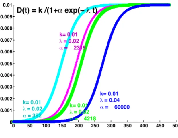
• for activated wounds (Figure 3): φ(t) = k
1 + α exp (−λt) (referred to as S-shaped)
0 50 100 150 200 250 300 350 400 450 500 0 0.001 0.002 0.003 0.004 0.005 0.006 0.007 0.008 0.009 0.01 k= 0.01 λ = 0.02 α = 2315 k= 0.01 λ = 0.04 α = 60000 k= 0.01 λ = 0.02 α = 4218 k= 0.01 λ = 0.02 α = 382 D(t) = k /(1+α exp(− λ t)
Figure 3: Illustration of S-shaped sigmoid profiles for activated wound closure φ(t) =1+α exp(−λt)k .
• for inhibited wounds (Figure 4): φ(t) =3k 2 −
k
C+ α exp (−λt) (referred to as Z-shaped).
The constant C should be close enough to 2/3 to allow for very low values for the approximated parameter at large time values. We denote by P = (k, λ, α) a generic set of variables which describes the sigmoid profile φ(t), by PD = (kD, λD, αD) the
one corresponding to the diffusion parameter D(t) and by Pr = (kr, λr, αr) the one
corresponding to the proliferation rate r(t). 2.3. Identification of the Fisher-KPP parameters
The most common validation methodology of mathematical models, notably for biological processes, amounts to use a portion of available experimental data to identify (or calibrate) the model parameters by minimizing some error cost function. Then use the model with calibrated parameters to predict the behavior of the modeled system, and then compare the predicted dynamics to the experimental ones.
Following the same methodology, let us denote by Ω the rectangular domain which defines the images frame, and by [T0, T ] the time window used to calibrate the model
parameters. This time window is a subset of the overall acquisition duration [0, TF]
where TFis the final available experimental data acquisition time.
Let us again formally denote by P the set of variables which describe the model parameters. For instance, if the Fisher-KPP parameters r and D are constant, then one may simply choose P = (r, D).
Let us denote by (uexp(t, x)) the sequence of experimental cell density images
(seg-mented and binarized), and let be the observation-error function JUdefined by
JU(P; u) = Z T T0 Z Ω |u(t, x) − uexp(t, x)|2dxdt.
0 50 100 150 200 250 300 350 400 450 500 0.005 0.006 0.007 0.008 0.009 0.01 0.011 0.012 0.013 0.014 0.015 k= 0.01 α =70 λ =0.08 k= 0.01 α =7000 λ =0.08 k=0.01 α=100 λ = 0.02 D(t) = (3k/2) − (k/(1+(α exp(−λt))) k=0.01 α = 382 λ = 0.02
Figure 4: Illustration of Z-shaped sigmoid profiles for inhibited wound closure φ(t) =3k2 − k
1+α exp(−λt).
where u = u(P) is the unique solution to the Fisher-KPP system (1)-(2)-(3)-(4) with model parameters described by P.
The identification problem amounts to find the P which minimizes, subject to spec-ified constraints, the following cost function j:
j(P) = JU(P ; u(P)) (5) The constraints are of bound (component-wise) type:
Pmin≤ P ≤ Pmax
The numerical values for the bounds are chosen so that the proliferation rate r(t) and collective diffusion coefficient D(t) lie into the largest interval known for these parameters : rmin≤ r(t) ≤ rmax and Dmin≤ D(t) ≤ Dmax. The migration rates for
MDCK cells in different settings (control, activation, inhibition) available from the literature, see e.g. [18], allow for the choice Dmin= 10−8and Dmax= 0.5. Considering,
from other part, doubling time bounds known for our biological experimental settings (from 10 hours to 2 or 3 days, for MDCK cells) allows to set a large bounds interval for the proliferation rate: rmin= 10−6 and rmax = 0.5. These considerations lead us
to set, in accordance, bounds for the sigmoid parameters. For the activated case, with S-shaped sigmoids, the magnitude of the parameters is as follows: 10−8≤ k, λ ≤ 0.5 and 10 ≤ α ≤ 103.
See the Section 3 below for the significance of the used units.
We refer the reader to [14] where we have extensively investigated, in the case where P = (r, D) are constant parameters, the profile of the cost function j and some tricky computational aspects of the minimization problem.
3. Results
3.1. The computational and validation settings
On original images, 1 pixel = 0.416 µm2= (0.645 µm)2, but due to computational restrictions on the image size, original images size is reduced by a rescaling factor of 8 × 8. On resized images, 1 pixel = 8 × 8 × 0.416 µm2, so the leading edge velocity and diffusion parameters units must be rescaled accordingly:
• Diffusion unit: 1 pixel.min−1= 1.6 10−3mm2.h−1= 1600 µm2.h−1 • Velocity unit: 1 pixel1/2.min−1= 309.10−3mm.h−1
Vexp(pixel1/2/min) is the experimental wound closure speed defined as the slope of
the linear regression w.r.t. time of the leading-edge (averaged in the i-coordinates) velocities;
Vcomp(pixel1/2/min) is the computed wound closure speed defined as for Vexp, using
the PDE model leading-edge evolution;
k (pixel/min), λ (min−1) and α (dimensionless) are the sigmoid optimal parameters; D (pixel/min) and r (min−1) are the proliferation rate and diffusion coefficient; J is the optimal relative cost function : we used J = JU/w0where w0is the initial
wound area (see Section 2.3 for the definition of JU);
[T0− T] (increments of 6 min) is the subset of images used to calibrate the model
parameters.
3.2. Fisher-KPP with constant parameters fails for activated or inhibited wound clo-sure
In order to highlight the need for a non constant parameters assumption, we recall herein the main results of our previous work in [14] obtained for the case of constant Fisher-KPP parameters.
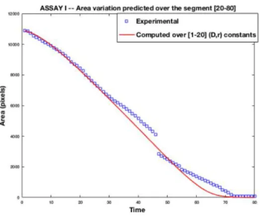
For control assays, Figure 5 shows a good accordance between the time evolution of the experimental wound area and the one of the computational model. Moreover, the experimental and the computed wound closure speeds are well approximated by the theoretical Fisher-KPP wavefront speed, that is known to be Vth= 2
√
rD(where (r, D) are the calibrated parameters, see [14] for details).
For activated assays, a high speed wound (Assay II, Figure 6), and an accelerating wound (Assay III, Figure 6), the mathematical model tries to fit the experimental data on the dataset window used for the calibration (that is the least expected by a calibration procedure), but is then unable to predict the time evolution of the wound area.
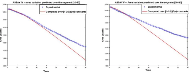
For inhibited assays, the mathematical model with the best calibrated parameters still closes the wound as shown in Figure 7 though with a small velocity, while the experimental assays do not.
Let us notice that the use, for the calibration, of the whole inhibited experimental dataset (that is, the whole segment [1-80] in our case) yields very small optimal values for the diffusion parameter D leading to the apparition of oscillations in the Fisher-KPP solutions (transition-to-chaos due to vanishing diffusion, see [14]).
Figure 5: The curve shows the area of the wound depending on time for sequence I (a reference one).
Figure 6: Time evolution of experimental versus computed wound area : (left) Assay II is an activated assay with leading edge high speed; (right) Assay III is an activated assay with accelerating leading edge. Results excerpt from [14].
3.3. Activated wound closure: D(t) is time dependent and r is constant
The diffusion parameter is postulated to be a time dependent S-shaped 3-parameter sigmoid as follows :
D(t) = k
1 + α exp(−λt), t→+∞lim D(t) = k. (6)
The proliferation rate r is taken as constant. Indeed, taking r a time dependent sigmoid does not outperform. For some calibration experiments instead, it counter-performs due to the double larger dimension of variables to deal with by the optimiza-tion procedure.
Figure 7: Time evolution of experimental versus computed wound area : (left) Assay IV and (right) Assay V are inhibited wounds. Results excerpt from [14].
3.3.1. Results for Assay II
Assay II is an activated assay with the wound leading edge which exhibits a high speed profile.
We have plotted in Figure 8 (left) the experimental and computed time evolution of the wound area. We also plotted the profile issued from the constant parameter assump-tion in order to highlight the advantage of taking time dependent diffusion parameter. The calibration is performed using different dataset windows, resulting in consistent calibrated area profiles and sigmoid parameters, see Table 1.
In Figure 8 (right), we plotted the experimental migration rate MRexp(pixel/min)
defined as the slope of the linear regression of the experimental wound area w.r.t. time. It is compared to the computed migration rate MRcomp defined as for MRexp, using
the PDE model area evolution. Figure 9 plots the sigmoidal time varying diffusion coefficient D(t) found for 3 different datasets used for the calibration.
Vexp Vcomp kD λD αD r T0− T J
0.067 0.072 0.02 0.0303 20 0.197 [1-20] 0.026113 0.089 0.095 0.02 0.04 29.998 0.1727 [1-34] 0.050088 0.085 0.089 0.02 0.0384 30 0.1847 [1-50] 0.052685
Table 1: Assay II : experimental vs computed velocities, and the optimally calibrated model parameters. Rows correspond to results computed over a dataset subset [T 0 − T ] of the overall [1 − 80] images.
3.3.2. Results for Assay III
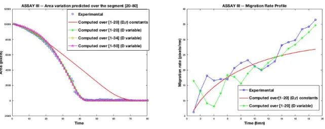
As for Assay II, the AssayIII is HGF activated, but with a slightly different dynam-ics. Indeed, from the Figure 10 (right) it can be observed that the wound closure shows
Figure 8: Assay II : time evolution of experimental versus computed wound area (left) and migration rate (right) for different dataset subsets used for the calibration, and the remaining used for the prediction. The area evolution and migration rate obtained with the calibration of constant parameters r and D are plotted in red line
–
.Figure 9: Assay II : sigmoid profiles of the diffusion parameter D(t) for different calibration datasets.
a kind of acceleration, with an increasing migration rate. It can be also observed in the same figure that the Fisher-KPP model with constant coefficients is not able to follow the experimental measures in the acceleration phase.
The evolution of the wound area presented in Figure 10 (left) corroborates this observation : at the beginning (sequences between 0 and 20 ) the constant and time-dependent calibrated parameters yield a wound area profile close to the experimental one. But, starting from sequence 30 to the closure, only the time-dependent calibrated parameters approximate well the experimental profile.
Figure 10: Assay III : time evolution of experimental versus computed wound area (left) and migration rate (right) for different dataset subsets used for the calibration, and the remaining used for the prediction. The area evolution and migration rate obtained with the calibration of constant parameters r and D are plotted in red line
–
.Figure 11: Assay III : sigmoid profiles of the diffusion parameter D(t) for different calibration datasets.
Table 2 shows the calibrated model parameters, which are quite consistent for the different used calibration datasets. Comparing the results in Table 1 to those of Table 2, one observes that λDand r have very comparable magnitudes (and also kDin some
sense), while the αD are very different, AssayIII alpha’s being about ten times those
of Assay II. Observing diffusion sigmoids, one remarks that the transition from low to high diffusion values occurs between 50 and 100 minutes for Assay II and between 100 and 150 minutes for Assay III.
If we write that :
αDexp(−λDt) = exp(λD(Tc− t)), where Tc=
ln(αD)
Vexp Vcomp kD λD αD r T0− T J
0.065 0.065 0.05 0.0383 343 0.2257 [1-20] 0.035925 0.099 0.102 0.05 0.0468 500 0.2084 [1-34] 0.059819 0.097 0.098 0.05 0.0497 588 0.2041 [1-50] 0.052438
Table 2: Assay III: Comparison of experimental and computed velocities for the optimally calibrated model parameters. Rows correspond to results computed over a dataset subset [T 0 − T ] of the overall [1 − 80] images.
(Tcmay be regarded as some activation characteristic time).
Computing average time Tcfor Assay II yields approximately 90 minutes, and for
Assay III approximately 137 minutes, which values are in concordance with the obser-vation above.
3.4. Inhibited wound closure: D(t) time dependent and r constant
The cell-sheets in the two assays : Assay IV and Assay V are treated with HGF and with a migration inhibitor LY29 (more precisely, L294002 which inhibits the PI3K signaling pathway).
For our MDCK cell-sheet inhibited wound closure, we postulate that the diffusion parameter D(t) in the Fisher-KPP equation can be approximated by a Z-shaped sigmoid profile as follows : D(t) =3kD 2 − kD C+ αDexp(−λDt) , C=2 3+ 10 −6, lim t→+∞D(t) ≈ 2.10 −6k D. (7)
The proliferation rate r is postulated as constant in time. Obviously, this assumption may be questionable from the biological point of view, nevertheless it turned out to be convenient enough for the capture of the wound closure behavior in the inhibition case, at least regarding the evolution of the leading edge and wound area. Actually, calibration experiments with sigmoid proliferation rates r(t) did not perform as well as the constant rate assumption : results presented in Table 5 show inconsistent parameters with respect to the dataset used for calibration, driving us to the conclusion that, in our opinion, the proliferation rate as a function of time should not be approximated using S-shaped or Z-shaped profiles.
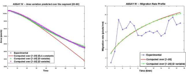
3.4.1. Results for Assay IV
After the initial wound scratch, the inhibited cell-sheet starts a migration phase for only a short while, then slows down until reaching a freezing of the leading edge. The Fisher-KPP model with constant parameters is not able to reproduce the freezing, yielding at some longer time a total closure, see Figure 12 (left). On the contrary, the model with a time-dependent diffusion coefficient is able to accurately follow the wound behavior, at least with respect to the evolution of the wound area.
It is also shown from Figure 12 (right) that the migration rate of the time-dependent case is very close to the one of the constant-parameter case, the two corresponding to
Figure 12: Assay IV : time evolution of experimental versus computed wound area (left) and migration rate (right) for different dataset subsets used for the calibration, and the remaining used for the prediction. The area evolution and migration rate obtained with the calibration of constant parameters r and D are plotted in red line
–
.the phase (on the sequences [1-20]) where the monolayer is in short time migration. So, with a time-dependent parameter, the model is able to capture both the initial migration phase as well as the inhibited leading edge freezing phase.
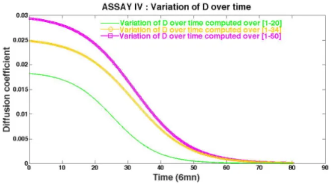
Figure 13 shows the calibrated sigmoid profiles of the diffusion parameter D(t) for different calibration datasets. Some consistency is observed with respect to these datasets. From Table 3 it is observed that the parameters kDand r are sensitive to the
used calibration dataset.
One may observe in Figure 12 (left) that the transition time interval in the Z-shaped profiles, around 30 (x6 minutes), corresponds to the time interval where the Fisher-KPP with constant (D, r) starts to slightly diverge away from the experimental wound evolution.
Vexp Vcomp kD λD αD r T0− T J
0.024 0.027 0.0124 0.025 30 0.0302 [1-20] 0.020981 0.030 0.030 0.0169 0.02 30 0.0237 [1-34] 0.033183 0.032 0.032 0.02 0.02 30 0.0207 [1-50] 0.046635
Table 3: Assay IV: Comparison of experimental and computed velocities for the optimally calibrated model parameters. Rows correspond to results computed over a dataset subset [T 0 − T ] of the overall [1 − 80] images.
3.4.2. Results for Assay V
In this inhibited Assay V, the initial migration phase is shorter than for Assay IV. Assay V exhibits an earlier freezing. In this case, it is observed from Figure 14 (left)
Figure 13: Assay IV : sigmoid profiles of the diffusion parameter D(t) for different calibration datasets.
Figure 14: Assay V : time evolution of experimental versus computed wound area (left) and migration rate (right) for different dataset subsets used for the calibration, and the remaining used for the prediction. The area evolution and migration rate obtained with the calibration of constant parameters r and D are plotted in red line
–
.Figure 15: Assay V : sigmoid profiles of the diffusion parameter D(t) for different calibration datasets.
that the deviation from the experimental wound area of the predicted Fisher-KPP with constant (D, r) parameters is much more pronounced with respect to the experience duration.
Figure 14 (right) shows that contrarily to the Assay IV, the migration rate of the time-dependent case deviates from the one of the constant-parameter case earlier (around 10x6 minutes) within the calibration dataset. Figure 15 shows the calibrated sigmoid profiles of the diffusion parameter D(t) for different calibration datasets. The Z-shape is stiffer and the profiles are more consistent than in the Assay IV case, as can also be seen from the numerical results in Table 4.
Vexp Vcomp kD λD αD r T0− T J
0.035 0.039 0.008 0.0562 30 0.0618 [1-20] 0.013133 0.034 0.038 0.008 0.04 30 0.0526 [1-34] 0.024598 0.033 0.035 0.008 0.04 50 0.0484 [1-50] 0.040999
Table 4: Assay V: Comparison of experimental and computed velocities for the optimally calibrated model parameters. Rows correspond to results computed over a dataset subset [T 0 − T ] of the overall [1 − 80] images.
3.5. Inhibited wound closure: the case of D(t) and r(t) sigmoidal time dependent profiles
It is observed from Figure 16 (left) that the calibration process is still able to provide a diffusion coefficient D(t) and a proliferation rate r(t) which yield a good prediction on the evolution of the wound area, much better than the one obtained with the constant (D, r) parameters assumption. The profiles of the respective migration rates seen from Figure 16 (right) are comparable to those obtained with r being not time-dependent. Indeed, it can be observed from Figure 17 that, while we have relaxed the ”r constant” assumption, the sigmoidal profiles for r tend to be flat enough to let r(t) behave as if it is a constant. Unfortunately, as may be seen from Figure 17 and from the numerical values in Table 5, the calibrated parameters dramatically depend on the dataset used
Figure 16: Assay IV : (left) Evolution of the wound area for 2 different calibration datasets for both D(t) and r(t) sigmoidal time-dependent, compared to the case (red line) of constant D and r parameters. (right) Experimental versus computed migration rate in case of time-dependent D(t) and r(t), compared to the case where the calibration is performed for constant (D, r) (plotted in red line
–
).for the calibration. In our opinion, this lack of consistency is due either to a locking phenomena (trying to fit a constant-wise parameter with a sigmoid function), or to the introduction of multiple minima. The two numerical pathologies could introduce the inconsistency behavior observed in the optimization procedure.
Vexp Vcomp kD λD αD kr λr αr T0− T J
0.024 0.027 0.0132 0.04 30 0.0204 0.007 40 [1-20] 0.020968 0.032 0.032 0.02 0.02 30 0.0143 0.007 40 [1-50] 0.046416
Table 5: Assay IV: Comparison of experimental and computed velocities for the optimally calibrated model parameters. Rows correspond to results computed over a dataset subset [T 0 − T ] of the overall [1 − 80] images.
4. Conclusion
We provided in [14] evidences that the 2D Fisher-KPP equation with constant dif-fusion and proliferation rate parameters fails to predict activated or inhibited cell-sheet wound closure. Thus, we considered in the present paper a 2D Fisher-KPP equation with a time dependent diffusion D(t) and a constant proliferation rate r. We used 3-parameter sigmoid approximation of D(t), with an S-shaped profile in case of ac-tivation, and a Z-shaped one in case of inhibition. We used a fraction (about 25%) of the available experimental dataset to calibrate the 3+1 diffusion and proliferation parameters, and the remaining of the dataset was used to assess the prediction ability
Figure 17: Assay IV : Profiles of D(t) and r(t) for the 2 different calibration datasets, showing inconsistency though the wound area variation approximate well the experimental one in both cases.
of the model. We then applied our method to two activated assays, one of them with high leading edge velocity and the other exhibiting a leading edge acceleration behav-ior, and to two inhibited assays. In both activated and inhibited settings, our model was able to predict with a good accuracy features of the wound closure like as the time evolution of the wound area and migration rate. The calibrated parameters were consistent with respect to different subsets of the experimental datasets used for the calibration. We also led calibration experiments where the proliferation rate r(t) was also taken time dependent sigmoid, but this assumption yielded sigmoid calibrated pa-rameters that were inconsistent with respect to the subset of the experimental dataset used for the calibration stage. Regarding this point, our conclusion is that, for the time duration of our assays, the time dependence of the proliferation rate is a less relevant assumption than for the diffusion coefficient.Finally, let us emphasize that the present study shows that one may keep in using the popular Fisher-KPP framework, which provides a simple formulation and a still rather easy 4-parameter characterization of the activated/inhibited cell motility.
5. References
[1] Alexandre J Kabla. Collective cell migration: leadership, invasion and segrega-tion. J R Soc Interface, 9(77):3268–78, December 2012.
[2] M. Poujade, E. Grasland-Mongrain, A. Hertzog, J. Jouanneau, P. Chavrier, B. Ladoux, A. Buguin, and P. Silberzan. Collective migration of an epithelial monolayer in response to a model wound. Proceedings of the National Academy of Sciences, 104(41):15988–15993, 2007.
[3] Gabriel Fenteany, Paul A. Janmey, and Thomas P. Stossel. Signaling pathways and cell mechanics involved in wound closure by epithelia cell sheets. Current Biology, 10(14):831–838, 2000.
[4] Qinghui Meng, James M. Mason, Debra Porti, Itzhak D. Goldberg, Eliot M. Rosen, and Saijun Fan. Hepatocyte growth factor decreases sensitivity to
chemotherapeutic agents and stimulates cell adhesion, invasion, and migration. Biochemical and Biophysical Research Communications, 274(3):772–779, 2000. [5] Eamonn A. Gaffney, Philip K. Maini, Jonathan A. Sherratt, and Paul D. Dale. Wound healing in the corneal epithelium: Biological mechanisms and mathemat-ical models. J. Theor. Med., 1(1):13–23, 1997.
[6] Karen M. Page, Philip K. Maini, and Nicholas A.M. Monk. Complex pattern for-mation in reaction-diffusion systems with spatially varying parameters. Physica D, 202(1-2):95–115, 2005.
[7] Julia C. Arciero, Qi Mi, Maria F. Branca, David J. Hackam, and David Swigon. Continuum model of collective cell migration in wound healing and colony ex-pansion. Biophysical Journal, 100(3):535 – 543, 2011.
[8] Luis Almeida, Patrizia Bagnerini, Abderrahmane Habbal, St´ephane Noselli, and Fanny Serman. A Mathematical Model for Dorsal Closure. Journal of Theoretical Biology, 268(1):105–119, January 2011.
[9] Nestor Sepulveda, Laurence Petitjean, Olivier Cochet, Erwan Grasland-Mongrain, Pascal Silberzan, and Vincent Hakim. Collective cell motion in an epithelial sheet can be quantitatively described by a stochastic interacting particle model. PLoS Comput Biol, 9(3), 2013.
[10] A. Kolmogoroff, I. Petrovsky, and N. Piscounoff. ´Etude de l’´equation de la dif-fusion avec croissance de la quantit´e de mati`ere et son application `a un probl`eme biologique. Bull. Univ. Etat Moscou, Ser. Int., Sect. A, Math. et Mecan. 1, Fasc. 6:1–25, 1937.
[11] R.A. Fisher. The wave of advance of advantageous genes. Annals of Eugenics, 7(4):355–369, 1937.
[12] P.K. Maini, D.L.S. McElwain, and D. Leavesley. Traveling waves in a wound healing assay. Appl. Math. Lett., 17(5):575–580, 2004.
[13] Matthew J. Simpson, Katrina K. Treloar, Benjamin J. Binder, Parvathi Haridas, Kerry J. Manton, David I. Leavesley, D. L. Sean McElwain, and Ruth E. Baker. Quantifying the roles of cell motility and cell proliferation in a circular barrier assay. Journal of The Royal Society Interface, 10(82), 2013.
[14] Abderrahmane Habbal, H´el`ene Barelli, and Gr´egoire Malandain. Assessing the ability of the 2D Fisher-KPP equation to model cell-sheet wound closure. Math. Biosci., 252:45–59, 2014.
[15] Assaf Zaritsky, Sari Natan, Eshel Ben-Jacob, and Ilan Tsarfaty. Emergence of hgf/sf-induced coordinated cellular motility. PLoS One, 7(9), 2012.
[16] Daniel F. Balkovetz. Hepatocyte growth factor and madin-darby canine kid-ney cells: In vitro models of epithelial cell movement and morphogenesis. Mi-croscopy Research and Technique, 43(5):456–463, 1998.
[17] Peng Liu, Bei Xu, Jianyong Li, and Hua Lu. {LY294002} inhibits leukemia cell invasion and migration through early growth response gene 1 induction indepen-dent of phosphatidylinositol 3-kinase-akt pathway. Biochemical and Biophysical Research Communications, 377(1):187 – 190, 2008.
[18] Julien Viaud, Mahel Zeghouf, H´el`ene Barelli, Jean-Christophe Zeeh, Andr´e Padilla, Bernard Guibert, Pierre Chardin, Catherine A. Royer, Jacqueline Cherfils, and Alain Chavanieu. Structure-based discovery of an inhibitor of arf activation by sec7 domains through targeting of protein-protein complexes. Proceedings of the National Academy of Sciences, 104(25):10370–10375, 2007.