HAL Id: hal-00166923
https://hal.archives-ouvertes.fr/hal-00166923
Preprint submitted on 12 Aug 2007
HAL is a multi-disciplinary open access
archive for the deposit and dissemination of
sci-entific research documents, whether they are
pub-lished or not. The documents may come from
teaching and research institutions in France or
abroad, or from public or private research centers.
L’archive ouverte pluridisciplinaire HAL, est
destinée au dépôt et à la diffusion de documents
scientifiques de niveau recherche, publiés ou non,
émanant des établissements d’enseignement et de
recherche français ou étrangers, des laboratoires
publics ou privés.
The solar photospheric abundance of phosphorus:
results from co5bold 3D model atmospheres
Elisabetta Caffau, Matthias Steffen, Luca Sbordone, Hans-G. Ludwig,
Piercarlo Bonifacio
To cite this version:
Elisabetta Caffau, Matthias Steffen, Luca Sbordone, Hans-G. Ludwig, Piercarlo Bonifacio. The solar
photospheric abundance of phosphorus: results from co5bold 3D model atmospheres. 2007.
�hal-00166923�
hal-00166923, version 1 - 12 Aug 2007
1(DOI: will be inserted by hand later) c
ESO 2007
Astronomy
&
Astrophysics
The solar photospheric abundance of phosphorus:
results from
CO
5BOLD
3D model atmospheres
E. Caffau
1, M. Steffen
2, L. Sbordone
1,3, H.-G. Ludwig
1,3, and P. Bonifacio
1,3,41 GEPI, Observatoire de Paris, CNRS, Universit´e Paris Diderot; Place Jules Janssen 92190 Meudon, France 2 Astrophysikalisches Institut Potsdam, An der Sternwarte 16, D-14482 Potsdam, Germany
3 CIFIST Marie Curie Excellence Team
4 Istituto Nazionale di Astrofisica, Osservatorio Astronomico di Trieste, Via Tiepolo 11, I-34143 Trieste, Italy
Received ...; Accepted ...
ABSTRACT
Aims.We determine the solar abundance of phosphorus using CO5BOLD 3D hydrodynamic model atmospheres.
Methods.High resolution, high signal-to-noise solar spectra of the P lines of Multiplet 1 at 1051-1068 nm are compared to line formation computations performed on a CO5BOLD solar model atmosphere.
Results.We find A(P)=5.46 ± 0.04, in good agreement with previous analysis based on 1D model atmospheres, due to the fact that the P lines of Mult. 1 are little affected by 3D effects. We cannot confirm an earlier claim by other authors of a downward revision of the solar P abundance by 0.1 dex employing a 3D model atmosphere.
Concerning other stars, we found modest (< 0.1 dex) 3D abundance corrections for P among four F-dwarf model atmospheres of different metallicity, being largest at lowest metallicity.
Conclusions.We conclude that 3D abundance corrections are generally rather small for the P lines studied in this work. They are marginally relevant for metal-poor stars, but may be neglected in the Sun.
Key words.Sun: abundances – Stars: abundances – Hydrodynamics
1. Introduction
Phosphorus is an element whose nucleosynthesis is not clearly understood and whose abundance is very poorly known out-side the solar system. It has a single stable isotope 31P, and
its most likely site of production are carbon and neon burning shells in the late stages of the evolution of massive stars, which end up as Type II SNe. The production mechanism is proba-bly through neutron capture, as it is for the parent nuclei29Si and30Si. According to Woosley & Weaver (1995) there is no significant P production during the explosive phases.
Like for other odd-Z elements (Na, Al) one expects that the P abundance should be proportional to the neutron excess η1. As metallicity decreases the neutron excess decreases and
these odd-Z elements should decrease more rapidly than neigh-Send offprint requests to: Elisabetta.Caffau@obspm.fr
1 as defined in Arnett (1971): η = (n
n−np)/(nn+ np), where nn
represents the total number of neutrons per gram, both free and bound in nuclei, and npthe corresponding number for protons
bouring even-Z elements. One can therefore expect decreasing [31P/30Si] or [31P/12Mg] with decreasing metallicity. Such a
be-haviour is in fact observed for Na (Andrievsky et al. 2007), however at low metallicity [Na/Mg] seems to reach a plateau at about [Na/Mg]∼ −0.5. One could expect a similar behaviour for P.
Phosphorus abundances in stars have so far been deter-mined for object classes not apt to study the chemical evolu-tion: chemically peculiar stars (e.g. Castelli et al. 1997; Fremat & Houziaux 1997, for a review of observations in Hg-Mn stars see Takada-Hidai 1991 and references therein), horizontal branch stars (Behr et al. 1999; Bonifacio et al. 1995; Baschek & Sargent 1976), sub-dwarf B type stars (Ohl et al. 2000; Baschek et al. 1982), Wolf-Rayet stars (Marcolino et al. 2007), PG 1159 stars (Jahn et al. 2007), and white dwarfs (Chayer et al. 2005; Dobbie et al. 2005; Vennes et al. 1996). Such stars are not useful to trace the chemical evolution because either they are chemically peculiar or they are evolved and may have changed their original chemical composition. A few
measure-2 Caffau et al.: Solar phosphorus abundance ments exist in O super-giants (Bouret et al. 2005; Crowther et
al. 2002) and B type stars (Tobin & Kaufmann 1984). Kato et al. (1996) measured P in Procyon, Sion et al. (1997) in the dwarf nova VW Hydri.
The abundance of P in F, G and K stars, which could be derived from the high excitation IR P lines of Mult. 1 at 1051–1068 nm has never been explored, due to the few high resolution near IR spectrographs available. With the advent of the CRIRES spectrograph at the VLT, the situation is likely to change and it will be possible to study the chemical evolution of P in the Galaxy using these long-lived stars as tracers. In this perspective it is interesting, as a reference, to revisit the solar P abundance in the light of the recent advances of 3D hydrody-namical model atmospheres. There are several determinations of the solar P abundance in the literature. Given the difficulty of this observation, it is not surprising that P was absent from the seminal work of Russell (1929). Lambert & Warner (1968) measured an abundance A(P)2 = 5.43, using 13 lines of P ,
of which four belong to Mult. 1 . The oscillator strength they used for these lines are very close to the Biemont & Grevesse (1973) values (see Table 3). Lambert & Luck (1978) measured A(P) = 5.45 ± 0.03, which is essentially the photospheric abun-dance adopted in the authoritative Anders & Grevesse (1989) compilation (A(P)= 5.45 ± 0.04). Based on their ab initio com-puted oscillator strengths Biemont et al. (1994) derived A(P) = 5.45 ± 0.06. With computed oscillator strengths, corrected to match measured energy level lifetimes, Berzinsh et al. (1997) derived 5.49 ± 0.04. In their compilation Grevesse & Sauval (1998) adopt A(P) = 5.45 ± 0.04. As can be seen, all de-terminations of the solar photospheric phosphorus abundance are in agreement, within the stated uncertainties. In disagree-ment with earlier work, Asplund et al. (2005) obtained a sig-nificantly lower value of A(P)= 5.36 ± 0.04 using a 3D solar model atmosphere computed with the Stein & Nordlund code (see Nordlund & Stein 1997). This result might be immediately interpreted as indication that 3D abundance corrections lead to a lower solar phosphorus abundance by ∼ 0.1 dex, but other factors, such as the choice of log g f values, can also explain this low A(P). The A(P) determinations found in literature are summarised in Table 2.
In the present paper we use a solar 3D CO5BOLD model to re-assess the solar phosphorus abundance. For comparison we also consider 1D solar models. Beyond the Sun, we further dis-cuss abundance corrections obtained for a number of F-dwarf models of varying metallicity.
2. Atomic data
We consider five IR P lines of Mult. 1 (see Table 1). Several determinations of the oscillator strengths for this multiplet are available in the literature (see Table 3). Generally, all values are rather close, differences are smaller than 0.1 dex for any
2 A(P) = log(N
P/NH) + 12
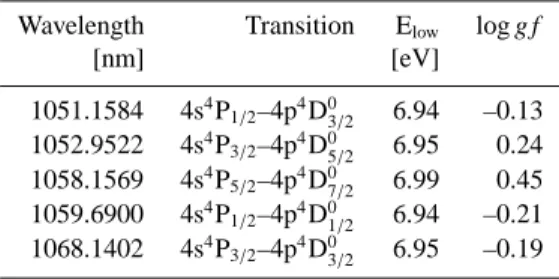
Table 1. Infra-red phosphorus lines considered in this work.
Wavelength Transition Elow log g f
[nm] [eV] 1051.1584 4s4P 1/2–4p4D03/2 6.94 –0.13 1052.9522 4s4P 3/2–4p4D05/2 6.95 0.24 1058.1569 4s4P 5/2–4p4D07/2 6.99 0.45 1059.6900 4s4P 1/2–4p4D01/2 6.94 –0.21 1068.1402 4s4P 3/2–4p4D03/2 6.95 –0.19
line except the 1051.2 nm line for which the maximum differ-ence is 0.18 dex. In this work we adopted the values computed by Berzinsh et al. (1997), corrected semi-empirically, which, in our opinion, are the best currently available. Had we cho-sen another set of values, with the notable exception of the Berzinsh et al. (1997) ab initio values, the difference in the derived phosphorus abundance would be 0.05 dex at most.
3. Models
Our analysis is based on a 3D model atmosphere computed with the CO5BOLD code (Freytag et al. 2002; Wedemeyer et al. 2004). In addition to the CO5BOLD hydrodynamical
sim-ulation we used several 1D models. More details about the em-ployed models can be found in Caffau et al. (2007) and Caffau & Ludwig (2007). In the following we will refer to the 1D model derived by a horizontal and temporal averaging of the 3D CO5BOLD model as the h3Di model. The reference 1D model for the computation of the 3D abundance corrections is a related (same Teff, log g, and chemical composition)
hy-drostatic 1D model atmosphere computed with the LHD code, hereafter 1DLHDmodel. LHD is a Lagrangian 1D
hydrodynam-ical model atmosphere code, which employs the same micro-physics as CO5BOLD. Convection is treated within the mixing-length approach. In the LHD model computation, as in any 1D theoretical atmosphere model, at least one free parameter de-scribing the treatment of convection must be decided upon: we use a mixing-length parameter of α=1.25 in the solar case, a value of α=1.8 in [M/H]=–2.0, and α=1.0 in [M/H]=–3.0 mod-els. We employ the formulation of Mihalas (1978) for mixing-length theory, and we neglect turbulent pressure in the momen-tum equation. We also considered the solar ATLAS 9 model computed by Fiorella Castelli 3 and the empirical
Holweger-M¨uller solar model (Holweger 1967; Holweger & Holweger-M¨uller 1974).
The spectrum synthesis codes employed are Linfor3D4for
all models, and SYNTHE (Kurucz 1993b, 2005a), in its Linux version (Sbordone et al. 2004; Sbordone 2005), for the fitting procedure with 1D or h3Di models. The advantage of using
3 http://wwwuser.oats.inaf.it/castelli/sun/ap00t5777g44377k1asp.dat 4 http://www.aip.de/ mst/Linfor3D/linfor 3D manual.pdf
SYNTHE, with respect to the present version of Linfor3D, is that it can handle easily a large number of lines, thus allowing to take into account numerous weak blends.
The 3D CO5BOLD solar model we used is the same we de-scribe in Caffau & Ludwig (2007). It covers a time interval of 6000 s, represented by 25 snapshots; this covers about 10 con-vective turn-over time scales, and 20 periods of the 5 minute os-cillations which are present in the 3D model as acoustic modes of the computational box.
Like in our study of sulphur (see Caffau & Ludwig 2007), we define as “3D abundance correction” the difference in the abundance derived from the full 3D model and the related 1DLHDmodel, in the sense A(3D) - A(1DLHD), both synthesised
with Linfor3D. We consider also the difference in the abun-dance derived from the 3D model and from the h3Di model. Since the 3D and h3Di models have, by construction, the same mean temperature structure, this allows to single out the effects due to the horizontal temperature fluctuations.
4. Data
As observational data we used two high-resolution, high signal-to-noise ratio spectra of disk-centre solar intensity: that of Neckel & Labs (1984) (hereafter referred to as the “Neckel intensity spectrum”) and that of Delbouille, Roland, Brault, & Testerman (1981) (hereafter referred to as the “Delbouille in-tensity spectrum”5). We also used the solar flux spectrum of
Neckel & Labs (1984) and the solar flux spectrum of Kurucz (2005)6, referred to as the “Kurucz flux spectrum”.
5. Data analysis
We measured the equivalent width (EW) of the lines using the IRAF task splot. We then computed the phosphorus abun-dance for the solar photosphere from the curve of growth of the line in question calculated with Linfor3D. As a confirma-tion of our results we fitted all observed line profiles with syn-thetic profiles. We found a good agreement in comparison to the abundances derived from the EWs. The remaining differ-ences we found are probably related to the difference in the continuum opacities used by SYNTHE with respect to the ones used by Linfor3D.
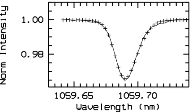
The line profile fitting was done using a code, described in Caffau et al. (2005), which performs a χ2 minimisation
of the deviation between synthetic profiles and the observed spectrum. Figure 1 shows the fit of the solar intensity spec-trum obtained from a grid of synthetic spectra synthesised with Linfor3D and based on the 3D CO5BOLD model. The close agreement between observed and synthetic line profile indi-cates that the non-thermal (turbulent) line broadening is very well represented by the hydrodynamical velocity field of the CO5BOLD simulation.
5 http://bass2000.obspm.fr/solaru spect.php 6 http://kurucz.harvard.edu/sun.html
Fig. 1. The observed disk-centre Neckel intensity spectrum (solid line) is plotted over the fit (crosses) obtained using a grid of synthetic spectra based on the CO5BOLD model computed with Linfor3D.
6. Results and discussion
6.1. The solar P abundance
The different sets of log g f values for the selected P lines are very close, so that the derived solar A(P) is quite insen-sitive to this choice. The solar phosphorus abundance varies by 0.05 dex, from the highest value obtained with the data set of Biemont et al. (1994) to the lower one obtained using Biemont & Grevesse (1973), the corrected value of Berzinsh et al. (1997), or the one from Kurucz & Peytremann (1975). A lower value of the solar phosphorus abundance (0.09 dex be-low the one obtained using the Biemont et al. (1994) oscillator strength) can be obtained using the non-corrected values from Berzinsh et al. (1997).
With the (corrected) log g f of Berzinsh et al. (1997) we obtain A(P)=5.443 ± 0.058 for the flux spectra considering the whole sample of five lines, A(P)=5.426±0.064 for the intensity spectra at disk-centre. The line at 1068.1 nm yields an abun-dance which is 1.6 σ below the mean value, while the other four lines are within one σ. If we remove this line from the compu-tation, the standard deviation drops by a factor of two and we obtain A(P)=5.467 ± 0.029, 5.450 ± 0.042 for flux and inten-sity spectra, respectively. The differences in the A(P) determi-nation from intensity and flux spectra could be due to NLTE corrections which usually are different in intensity and flux. Unfortunately, there are no NLTE computations available for these lines. Our recommended solar photospheric abundance is A(P)=5.458 ± 0.036, very close to all previous 1D determina-tions, however 0.1 dex higher than the value found by Asplund et al. (2005) using a 3D model.
The result of Asplund et al. (2005) is difficult to interpret since, according to our model, the 3D corrections for the P lines in the Sun are small. Asplund et al. (2005) do not pro-vide detailed information on the lines used or of their adopted EWs. They adopted the log g f of Berzinsh et al. (1997), how-ever they do not specify if they used the “corrected” or ab initio values. If they used the ab initio values the difference is easily
4 Caffau et al.: Solar phosphorus abundance -4 -2 0 2 4 6 log10τ 0.00 0.02 0.04 0.06 0.08 0.10 ∆ TRMS /<T>
Fig. 2. Relative horizontal RMS temperature fluctuations (on surfaces of equal Rosseland optical depth) in the solar CO5BOLD model.
understood, otherwise we must conclude that the difference is due either to a difference between their 3D simulation and the CO5BOLD one, or due to a difference in the adopted EWs. We point out here that our measured EWs are in quite good agree-ment with both those of Lambert & Warner (1968), Lambert & Luck (1978) and with those of Biemont et al. (1994)
A detailed summary of the solar phosphorus abundances we derived from individual lines, using different model atmo-spheres, in given in Table 4. Since the considered lines are not truly weak, the 3D corrections are unfortunately sensitive to the adopted micro-turbulence, and hence must be interpreted with care. The 3D corrections due to horizontal temperature fluctu-ations only, indicated by the 3D-h3Di difference, are slightly positive throughout. In all lines, the 3D-h3Di difference for in-tensity spectra is systematically higher than for flux spectra, by roughly 0.02 dex. This is presumably due to the fact that the intensity spectra originate from somewhat deeper layers where horizontal fluctuations are larger. We note that the phosphorus lines are formed mostly in the range −0.5 < log10τross < 0,
where the horizontal temperature fluctuations increase with in-creasing optical depth (see Fig. 2).
The 3D-h3Di difference increases with the excitation po-tential of the line’s lower level. In fact, the 3D-h3Di correction is rather small, not exceeding +0.030 dex for ξ=1.0 km s−1, and
+0.045 dex for ξ=1.5 km s−1, which we consider as an upper
limit.
The 3D-1DLHD corrections are systematically larger than
the 3D-h3Di difference (by +0.01 to 0.02 dex), but of the same order of magnitude. From that we can conclude that the solar h3Di and 1DLHDtemperature profiles are very similar.
6.2. 3D effects on P for other stars.
As shown above, we obtain only mild 3D effects in our solar phosphorus abundance analysis. They are comparable to the standard deviation (as listed in col. (9) of Table 4) for the weak
lines, and a factor four larger than the standard deviation for the strongest line, and hence the 3D effects are hardly relevant. However, 3D effects should become stronger for metal-poor stars where the temperature profiles differ more strongly be-tween h3Di and 1DLHDmodels than for solar metallicity
mod-els (Asplund 2005). Very little work has been dedicated to 3D effects on the phosphorus abundance, and none for metal-poor stellar models. To check the behaviour of the 3D abundance corrections, we theoretically investigated for a few available 3D CO5BOLD models the phosphorus 3D-1D
LHD relation in
the resulting synthetic flux spectra.
We find, for three metal-poor models (6300/4.5/–2.07; 5900/4.5/–3.0; 6500/4.5/–3.0), that the difference in the mean temperature profile is the only factor which contributes to the 3D correction. In the metal-poor models, as in the solar model, the maximum contribution to the equivalent widths of the P lines comes from a well defined region close to the continuum forming layers. Even though the optical depth range contribut-ing significantly is somewhat broader in the metal-poor models than in the solar model, the h3Di and 1DLHDmodels are
usu-ally rather close in temperature in this region, and so the effects of the different mean temperature structure are not very pro-nounced for the considered P lines. The 3D correction related to the difference in the mean temperature structure of the 3D and 1DLHDmodel amounts to ≈ +0.05 dex for the –2.0
metal-licity model, and to ≈ +0.1 dex for the most metal-poor model. For a 3D CO5BOLD model of Procyon (6500/4.0/0.0) the difference in the temperature profile of the h3Di and 1DLHD
model contributes to more than half of the total 3D correction. In Procyon, P lines are formed at shallower optical depths than in the Sun by about ∆ log τ ≈ 0.3. In this range the 1DLHDmodel is cooler than the 3D CO5BOLD one. The
re-lated abundance correction depends on the excitation poten-tial (strength) of the line, and for the strongest line it is still less than +0.030 dex. The contribution to the 3D correction related to the horizontal temperature fluctuations ranges from +0.022 to +0.045 dex, increasing with the excitation potential (strength) of the line. In the range where the line is formed, the horizontal RMS temperature fluctuations in Procyon are of the order of 5% to be compared to 1% in the metal-poor models. The total 3D correction is thus less than +0.07 dex for all lines.
7. Conclusions
Using the CO5BOLD solar granulation model, we have de-termined the solar 3D LTE phosphorus abundance to be A(P)=5.46±0.04, which compares very well to all previous de-terminations obtained using 1D models. This can be explained by the fact that the P lines of Mult. 1 appear to be rather in-sensitive to granulation effects, at least in the parameter inter-val explored by us (F and G dwarfs of metallicity from solar to –3.0). These lines can thus be useful to investigate the
chem-7 indicating T
ical evolution of phosphorus in the Galactic disk and in mod-erately metal-poor environments. Below [P/H]=–1.0, however, the lines have EWs smaller than 0.5 pm, becoming exceedingly difficult to observe.
For the P lines studied in this work, we find small (Sun) to moderate (Procyon, metal-poor stars) 3D abundance correc-tions. The sign of the corrections is found to be positive in all cases, meaning that the abundances resulting from a 3D analy-sis are larger than those obtained from a 1D model. Note that this behaviour is consistent with the results obtained by Steffen & Holweger (2002) for S , which has almost the same ionisa-tion potential as P (see their Fig. 8). In general, however, the magnitude and sign of the 3D effects depend on the properties of the absorbing ion (ionisation potential, the excitation poten-tial of the lower level, line strength and wavelength), and on the thermodynamic structure of the stellar atmosphere. The results obtained in this work for P must therefore not be generalised to other elements and other types of stars.
Acknowledgements. The authors L.S., H.-G.L., P.B. acknowledge
fi-nancial support from EU contract MEXT-CT-2004-014265 (CIFIST). We acknowledge use of supercomputing centre CINECA, which has granted us time to compute part of the hydrodynamical models used in this investigation, through the INAF-CINECA agreement 2006,2007.
References
Aller, L. H. 1949, ApJ, 109, 244
Anders, E., & Grevesse, N. 1989, Geochim. Cosmochim. Acta, 53, 197
Andrievsky, S. M., Spite, M., Korotin, S. A., Spite, F., Bonifacio, P., Cayrel, R., Hill, V., & Franc¸ois, P. 2007, A&A, 464, 1081
Arnett, W. D. 1971, ApJ, 166, 153 Asplund, M. 2005, ARA&A, 43, 481
Asplund, M., Grevesse, N., & Sauval, A. J. 2005, ASP Conf. Ser. 336: Cosmic Abundances as Records of Stellar Evolution and Nucleosynthesis, 336, 25
Baschek, B., Scholz, M., Kudritzki, R. P., & Simon, K. P. 1982, A&A, 108, 387
Baschek, B., & Sargent, A. I. 1976, A&A, 53, 47
Behr, B. B., Cohen, J. G., McCarthy, J. K., & Djorgovski, S. G. 1999, ApJ, 517, L135
Berzinsh, U., Svanberg, S., & Biemont, E. 1997, A&A, 326, 412
Biemont, E., Martin, F., Quinet, P., & Zeippen, C. J. 1994, A&A, 283, 339
Biemont, E. and Grevesse, N. 1973, At. Data Nucl. Data Tables 12, 217
Bonifacio, P., Castelli, F., & Hack, M. 1995, A&AS, 110, 441 Bouret, J.-C., Lanz, T., & Hillier, D. J. 2005, A&A, 438, 301 Caffau, E., & Ludwig, H.-G. 2007, A&A, 467, L11
Caffau, E., Bonifacio, P., Faraggiana, R., Franc¸ois, P., Gratton, R. G., & Barbieri, M. 2005, A&A, 441, 533
Caffau, E., Faraggiana, R., Bonifacio, P., Ludwig, H.-G., & Steffen, M. 2007, A&A, 470, 699
Castelli, F., Parthasarathy, M., & Hack, M. 1997, A&A, 321, 254
Chayer, P., Vennes, S., Dupuis, J., & Kruk, J. W. 2005, ApJ, 630, L169
Crowther, P. A., Hillier, D. J., Evans, C. J., Fullerton, A. W., De Marco, O., & Willis, A. J. 2002, ApJ, 579, 774
Dobbie, P. D., Barstow, M. A., Hubeny, I., Holberg, J. B., Burleigh, M. R., & Forbes, A. E. 2005, MNRAS, 363, 763 Fremat, Y., & Houziaux, L. 1997, A&A, 320, 580
Freytag, B., Steffen, M., & Dorch, B. 2002, AN, 323, 213 Garcia, Z. L., & Levato, H. 1986, Astrophys. Lett., 25, 1 Grevesse, N., & Sauval, A. J. 1998, Space Science Reviews,
85, 161
Holweger, H. 1967, Zeitschrift f¨ur Astrophysik, 65, 365 Holweger, H., & Mueller, E. A. 1974, Sol. Phys., 39, 19 Jahn, D., Rauch, T., Reiff, E., Werner, K., Kruk, J. W., &
Herwig, F. 2007, A&A, 462, 281
Kato, K.-I., Watanabe, Y., & Sadakane, K. 1996, PASJ, 48, 601 Kaufmann, J. P., & Schonberger, D. 1977, A&A, 57, 169 Kurucz, R. 1993b, SYNTHE Spectrum Synthesis Programs
and Line Data. Kurucz CD-ROM No. 18. Cambridge, Mass.: Smithsonian Astrophysical Observatory, 1993., 18
Kurucz, R. L. 2005a, MSAIS, 8, 14 Kurucz, R. L. 2005, MSAIS, 8, 189
Kurucz, R. L., & Peytremann, E. 1975, SAO Special Report, 362
Lambert, D. L., & Warner, B. 1968, MNRAS, 138, 181 Lambert, D. L., & Luck, R. E. 1978, MNRAS, 183, 79 Marcolino, W. L. F., Hillier, D. J., de Araujo, F. X., & Pereira,
C. B. 2007, ApJ, 654, 1068
Mihalas, D. 1978, San Francisco, W. H. Freeman and Co., 1978. 650 p.
Neckel, H., & Labs, D. 1984, Sol. Phys., 90, 205
Nordlund, A., & Stein, R. 1997, SCORe’96 : Solar Convection and Oscillations and their Relationship, 225, 79
Ohl, R. G., Chayer, P., & Moos, H. W. 2000, ApJ, 538, L95 Russell, H. N. 1929, ApJ, 70, 11
Sbordone, L. 2005, MSAIS, 8, 61
Sbordone, L., Bonifacio, P., Castelli, F., & Kurucz, R. L. 2004, MSAIS, 5, 93
Seligman, C. E., & Aller, L. H. 1970, Ap&SS, 9, 461
Sion, E. M., Cheng, F. H., Sparks, W. M., Szkody, P., Huang, M., & Hubeny, I. 1997, ApJ, 480, L17
Steffen, M., & Holweger, H. 2002, A&A, 387, 258
Takada-Hidai, M. 1991, IAU Symp. 145: Evolution of Stars: the Photospheric Abundance Connection, 145, 137
Tobin, W., & Kaufmann, J. P. 1984, MNRAS, 207, 369 Vennes, S., Chayer, P., Hurwitz, M., & Bowyer, S. 1996, ApJ,
468, 898
Wedemeyer, S., Freytag, B., Steffen, M., Ludwig, H.-G., & Holweger, H. 2004, A&A, 414, 1121
Caffau et al.: Solar phosphorus abundance, Online Material p 1
Caffau et al.: Solar phosphorus abundance, Online Material p 2 Table 2. Spectroscopic determinations of the solar
photo-spheric phosphorus abundance.
A(P) σ Reference
5.43 Lambert & Warner (1968) 5.45 0.03 Lambert & Luck (1978) 5.45 0.04 Anders & Grevesse (1989) 5.45 0.06 Biemont et al. (1994) 5.49 0.04 Berzinsh et al. (1997) 5.45 0.04 Grevesse & Sauval (1998) 5.36 0.04 Asplund et al. (2005) 5.46 0.04 this work
Table 3. Oscillator strength for the IR phosphorus lines (wave-lengths in nm) available in the literature.
log g f Reference 1051.2 1053.0 1058.2 1059.7 1068.1
–0.21 0.20 0.48 –0.21 –0.10 Kurucz & Peytremann (1975) –0.23 0.18 –0.24 –0.12 NIST
–0.06 0.31 0.52 –0.14 –0.12 Berzinsh et al. (1997) –0.13 0.24 0.45 –0.21 –0.19 Berzinsh et al. (1997) corr. –0.10 0.27 0.49 –0.17 –0.15 Biemont et al. (1994) –0.24 0.17 0.45 –0.24 –0.13 Biemont & Grevesse (1973)
Caffau et al.: Solar phosphorus abundance, Online Material p 3
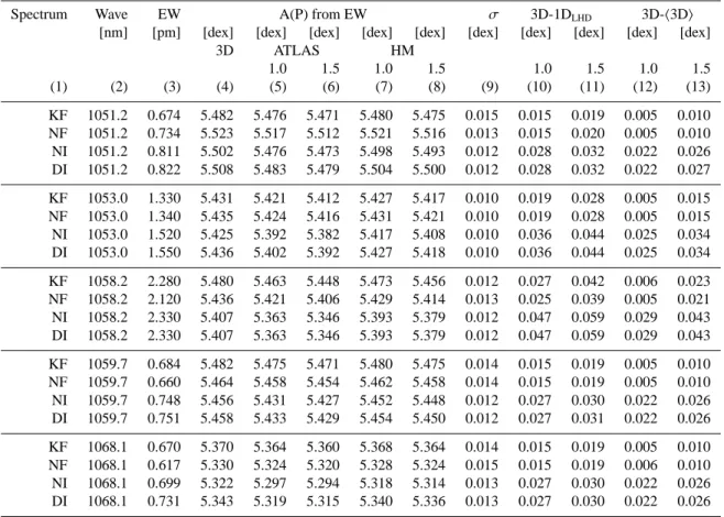
Table 4. Solar phosphorus abundances from the various observed spectra, adopting the (corrected) log g f of Berzinsh et al. (1997).
Spectrum Wave EW A(P) from EW σ 3D-1DLHD 3D-h3Di
[nm] [pm] [dex] [dex] [dex] [dex] [dex] [dex] [dex] [dex] [dex] [dex]
3D ATLAS HM 1.0 1.5 1.0 1.5 1.0 1.5 1.0 1.5 (1) (2) (3) (4) (5) (6) (7) (8) (9) (10) (11) (12) (13) KF 1051.2 0.674 5.482 5.476 5.471 5.480 5.475 0.015 0.015 0.019 0.005 0.010 NF 1051.2 0.734 5.523 5.517 5.512 5.521 5.516 0.013 0.015 0.020 0.005 0.010 NI 1051.2 0.811 5.502 5.476 5.473 5.498 5.493 0.012 0.028 0.032 0.022 0.026 DI 1051.2 0.822 5.508 5.483 5.479 5.504 5.500 0.012 0.028 0.032 0.022 0.027 KF 1053.0 1.330 5.431 5.421 5.412 5.427 5.417 0.010 0.019 0.028 0.005 0.015 NF 1053.0 1.340 5.435 5.424 5.416 5.431 5.421 0.010 0.019 0.028 0.005 0.015 NI 1053.0 1.520 5.425 5.392 5.382 5.417 5.408 0.010 0.036 0.044 0.025 0.034 DI 1053.0 1.550 5.436 5.402 5.392 5.427 5.418 0.010 0.036 0.044 0.025 0.034 KF 1058.2 2.280 5.480 5.463 5.448 5.473 5.456 0.012 0.027 0.042 0.006 0.023 NF 1058.2 2.120 5.436 5.421 5.406 5.429 5.414 0.013 0.025 0.039 0.005 0.021 NI 1058.2 2.330 5.407 5.363 5.346 5.393 5.379 0.012 0.047 0.059 0.029 0.043 DI 1058.2 2.330 5.407 5.363 5.346 5.393 5.379 0.012 0.047 0.059 0.029 0.043 KF 1059.7 0.684 5.482 5.475 5.471 5.480 5.475 0.014 0.015 0.019 0.005 0.010 NF 1059.7 0.660 5.464 5.458 5.454 5.462 5.458 0.014 0.015 0.019 0.005 0.010 NI 1059.7 0.748 5.456 5.431 5.427 5.452 5.448 0.012 0.027 0.030 0.022 0.026 DI 1059.7 0.751 5.458 5.433 5.429 5.454 5.450 0.012 0.027 0.031 0.022 0.026 KF 1068.1 0.670 5.370 5.364 5.360 5.368 5.364 0.014 0.015 0.019 0.005 0.010 NF 1068.1 0.617 5.330 5.324 5.320 5.328 5.324 0.015 0.015 0.019 0.006 0.010 NI 1068.1 0.699 5.322 5.297 5.294 5.318 5.314 0.013 0.027 0.030 0.022 0.026 DI 1068.1 0.731 5.343 5.319 5.315 5.340 5.336 0.013 0.027 0.030 0.022 0.026
Col. (1) spectrum identification: DI: Delbouille intensity, NI: Neckel intensity, NF: Neckel flux, KF: Kurucz flux. Col. (2) wavelength of the line. Col. (3) measured equivalent width. Col. (4) phosphorus abundance, A(P), according to the CO5BOLD 3D model. Cols. (5)-(8) provide A(P) from 1D models, odd numbered cols. correspond to a micro-turbulence ξ of 1.0 km s−1, even numbered cols. to ξ = 1.5 km s−1. Col. (9)
uncertainty in A(P) due to the uncertainty in the measured EWs. Col. (10)-(13) provide 3D corrections, even numbered cols. for ξ = 1.0 km s−1,