Deviation magnification: Revealing departures from ideal geometries

Deviation magnification: Revealing

departures from ideal geometries

The MIT Faculty has made this article openly available.

Please share

how this access benefits you. Your story matters.

Citation

Neal Wadhwa, Tali Dekel, Donglai Wei, Fredo Durand, and William

T. Freeman. 2015. Deviation magnification: revealing departures

from ideal geometries. ACM Trans. Graph. 34, 6, Article 226 (October

2015), 10 pages.

As Published

http://dx.doi.org/10.1145/2816795.2818109

Publisher

Association for Computing Machinery (ACM)

Version

Author's final manuscript

Citable link

http://hdl.handle.net/1721.1/99938

Terms of Use

Creative Commons Attribution-Noncommercial-Share Alike

ACM Reference Format

Wadhwa, N., Dekel, T., Wei, D., Durand, F., Freeman, W. 2015. Deviation Magnifi cation: Revealing Depar-tures from Ideal Geometries. ACM Trans. Graph. 34, 6, Article 226 (November 2015), 10 pages. DOI = 10.1145/2816795.2818109 http://doi.acm.org/10.1145/2816795.2818109.

Copyright Notice

Permission to make digital or hard copies of part or all of this work for personal or classroom use is granted without fee provided that copies are not made or distributed for profi t or commercial advantage and that cop-ies bear this notice and the full citation on the fi rst page. Copyrights for third-party components of this work must be honored. For all other uses, contact the Owner/Author.

Copyright held by the Owner/Author.

SIGGRAPH Asia ‘15 Technical Paper, November 02 – 05, 2015, Kobe, Japan. ACM 978-1-4503-3931-5/15/11.

DOI: http://doi.acm.org/10.1145/2816795.2818109

Deviation Magnification: Revealing Departures from Ideal Geometries

Neal Wadhwa Tali Dekel Donglai Wei Fr´edo Durand William T. Freeman

MIT Computer Science and Artificial Intelligence Laboratory

(a) Input Image

View I

View II

(for verfication only)

Views processed independently by Deviation Magnification

(c) Input Image (d) Our Result

p

p

p

p

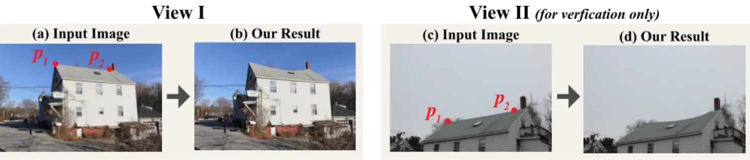
Figure 1: Revealing the sagging of a house’s roof from a single image. A perfect straight line marked by p1andp2is automatically fitted to the house’s roof in the input image (a). Our algorithm analyzes and amplifies the geometric deviations from straight, revealing the sagging of the roof in (b). View II shows a consistent result of our method (d) using another image of the same house from a different viewpoint (c). Each viewpoint was processed completelyindependently.

Abstract

Structures and objects are often supposed to have idealized geome-tries such as straight lines or circles. Although not always visible to the naked eye, in reality, these objects deviate from their idealized models. Our goal is to reveal and visualize such subtle geometric deviations, which can contain useful, surprising information about our world. Our framework, termed Deviation Magnification, takes a still image as input, fits parametric models to objects of interest, computes the geometric deviations, and renders an output image in which the departures from ideal geometries are exaggerated. We demonstrate the correctness and usefulness of our method through quantitative evaluation on a synthetic dataset and by application to challenging natural images.

CR Categories: I.4.8 [Image Processing and Computer Vision]: Scene Analysis—Shape;

Keywords: deviation, geometry, magnification

1

Introduction

Many phenomena are characterized by an idealized geometry. For example, in ideal conditions, a soap bubble will appear to be a perfect circle due to surface tension, buildings will be straight and planetary rings will form perfect elliptical orbits. In reality, how-ever, such flawless behavior hardly exists, and even when invisible to the naked eye, objects depart from their idealized models. In the presence of gravity, the bubble may be slightly oval, the build-ing may start to sag or tilt, and the rbuild-ings may have slight

perturba-tions due to interacperturba-tions with nearby moons. We present Deviation Magnification, a tool to estimate and visualize such subtle geomet-ric deviations, given only a single image as input. The output of our algorithm is a new image in which the deviations from ideal are magnified. Our algorithm can be used to reveal interesting and important information about the objects in the scene and their in-teraction with the environment. Figure 1 shows two independently processed images of the same house, in which our method auto-matically reveals the sagging of the house’s roof, by estimating its departure from a straight line.

Our approach is to first fit ideal geometric models, such as lines, cir-cles and ellipses, to objects in the input image, and then look at the residual from the fit, rather than the fit itself. This residual is then processed and amplified to reveal the physical geometric departure of the object from its idealized shape. This approach of model fit-ting followed by processing of the residual signal is in the spirit of recent methods for motion magnification [Wu et al. 2012; Wadhwa et al. 2013]. These methods magnify small motions over time, re-vealing deviations from perfect stationarity in nearly still video se-quence. Here, however, we are interested in deviations over space from canonical geometric forms, using only a single image. Our algorithm serves as a microscope for form deviations and is appli-cable regardless of the time history of the changes. For example, we can exaggerate the sag of a roof line from only a single photo without any prior knowledge on what it looked like when it was built or how it changed over time. The important information is the departure from the canonical shape.

Finding the departures from the fitted model is not trivial. They are often very subtle (less than a pixel in some applications), and can be confused with non-geometric sources of deviations, such as image texture on the object. Our algorithm addresses these issues by combining careful sub-pixel sampling, reasoning about spatial aliasing, and image matting. Matting produces an alpha matte that matches the object’s edge to sub-pixel accuracy. Therefore, oper-ating on the alpha matte allows us to preserve the deviation signal while removing texture. The deviation signal is then obtained by estimating small changes in the alpha matte’s values, perpendicular to the contour of the shape. The resulting framework is generic, and is independent of the number or type of fitted shape models.

Input Image

(3) Analysis (4) Synthesis

Synthesize Magnified Image Generate Deformation Field Sampling edge profiles orthogonal to L

x p₁ pj p₂ Filtered Deviation (2) Canonical Stripe L p₁ p₂ p_jn n Sampling n Matting n

Edge profiles, S(pi), in the normal direction ( ) S(p1)S(pj) model edge Sm S(p2) (1) Geometry Fitting L p1 p2 p2 p1

Intensity along the fitted line L

Deviation from Sm

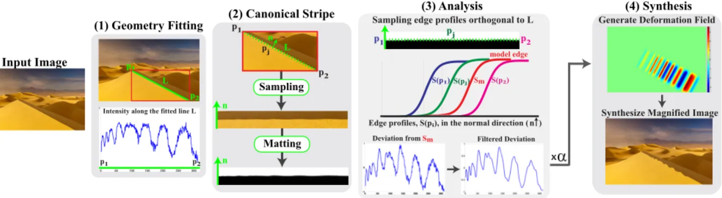
Figure 2: Outline of Deviation Magnification: a parametric shape (e.g., a line segment) is fitted to the input image (either automatically or with user interaction). The region near the contour of the shape is sampled and transformed into a canonical stripe representation. The alpha matte of the stripe is then computed using [Levin et al. 2008] and then fed into the analysis step. In this step, deviation from the fitted shape is computed: the edge profilesS(pj) in the vertical direction are sampled for each location pj along the stripe, and a model edge profileSmis estimated; the 1D translation between the edge profilesS(pj) and Smis estimated to form the deviation signal. The filtered deviation signal is then magnified by a factor ofα and used to generate a deformation field. The synthesized image is rendered accordingly and reveals the spatial deviation from the fitted shape. In this case, the periodic ripples of the sand dune ridge are revealed. (Image courtesy of Jon Cornforth.)

In many cases, the deviation signals are invisible to the naked eye. Thus, to verify that they are indeed factual, we conducted a com-prehensive evaluation using synthetic data with known ground truth as well as controlled experiments using real world data. We demon-strate the use of Deviation Magnification on a wide range of appli-cations in engineering, geology and astronomy. Examples include revealing invisible tilting of a tower, nearly invisible ripple marks on a sand dune and distortions in the rings of Saturn.

2

Related Work

Viewed very generally, some common processing algorithms can be viewed as deviation magnification. In unsharp masking, a blurred version of an image is used as a model and deviations from the model are amplified to produce a sharpened image. Facial carica-tures are another example of this kind of processing, in which the deviations of a face image from an idealized model, the mean face, are amplified [Blanz and Vetter 1999].

Motion magnification [Liu et al. 2005; Wadhwa et al. 2013; Wad-hwa et al. 2014; Wu et al. 2012; Elgharib et al. 2015] uses the same paradigm of revealing the deviations from a model. However, there is no need to detect the model as the direction of time is readily given. In addition, motion magnification assumes that objects are nearly static i.e. the appearance over time is assumed to be nearly constant. In contrast, our technique amplifies deviations from a general spatial curve detected in a single image. The type and lo-cation of this curve depends on the applilo-cation, and the appearance along it may change dramatically posing new challenges for our problem.

A recent, related method was presented for revealing and estimat-ing internal non parametric variations within an image [Dekel et al. 2015]. This method assumes that the image contains recurring pat-terns, and reveals their deviation from perfect recurrence. This is done by estimating an “ideal” image that has stronger repetitions and a transformation that brings the input image closer to ideal. In contrast, our method relies on parametric shapes within the image, and thus can be applied for images that do not have recurring struc-tures. Our parametric approach allows our algorithm to accurately reveal very tiny, nearly invisible deviations, which cannot be esti-mated by Dekel et al. [2015].

Our method relies on detecting and localizing edges, a problem for which many techniques have been proposed (e.g. [Duda and Hart 1972; P˘atr˘aucean et al. 2012; Fischler and Bolles 1981]). One class of techniques uses the observation that edges occur at locations of steepest intensity and are therefore well-characterized by the peak of derivative filters of the image (e.g. [Canny 1986; Nalwa and Binford 1986; Freeman and Adelson 1991]). More recently, several authors have applied learning techniques to the problem of edge de-tection to better distinguish texture from edges (e.g. [Dollar et al. 2006; Lim et al. 2013; Doll´ar and Zitnick 2013]). Because the de-viations in the images we seek to process are so small, we obtained good results adopting a flow-based method, similar to Lucas and Kanade [1981]. Since texture variations can influence the detected edge location, we used image matting [Levin et al. 2008] to remove them.

3

Method

Our goal is to reveal and magnify small deviations of objects from their idealized elementary shapes given a single input image.

3.1 Overview

There are four main steps in our method, illustrated in Figure 2. The first step of our algorithm is to detect elementary shapes, i.e., lines, circles, and ellipses, in the input image. This can be performed completely automatically by applying an off-the-shelf fitting algo-rithm (e.g., [P˘atr˘aucean et al. 2012]) to detect all the elementary shapes in the image. Alternatively, it can be performed with user interaction as discussed in Section 3.5. The detected shapes serve as the models from which deviations are computed.

With the estimated models in hand, we opt to perform a generic spa-tial analysis, independent of the number and type of fitted shapes. To this end, the local region around each shape is transformed to a canonical image stripe (Figure 2(3)). In this representation, the contour of the shape becomes a horizontal line and the local normal direction is aligned with the vertical axis. To reduce the impact of imperfections that are caused by image texture and noise, a matting algorithm is applied on each of the canonical stripes. This step sig-nificantly improves the signal-to-noise ratio, and allows us to deal

with real world scenarios, as demonstrated in our experiments. Each canonical matte is analyzed, and its edge’s deviation from a perfectly horizontal edge is estimated. This is done by computing 1D translations between vertical slices in the matted stripe, assum-ing these slices have the same shape along the stripe. For each canonical matte, this processing yields a deviation signal that cor-responds to the deviation from the associated model shape in the original image, in the local normal direction. Depending on the ap-plication, the deviation signals may be low-passed or bandpassed with user-specified cutoffs, allowing us to isolate the deviation of interest.

Lastly, the computed deviation signals are visually revealed by ren-dering a new image in which the deviations are magnified. Specif-ically, a 2D deformation field is generated based on the 1D com-puted deviation signals, and is then used to warp the input image. We next describe these steps in more detail.

3.2 Deviations from a Parametric Shape

Consider a synthetic image I(x, y), shown in Figure 3(a), which has an edge along the x-axis as a model of a matted image stripe. This edge appears to be perfectly horizontal, but actually has a subtle deviation from straight (shown twenty times larger in Fig-ure 3(b)). Our goal is to estimate this deviation signal f (x), at every location x along the edge.

To do this, we look at vertical slices or edge profiles of the image I, e.g. the intensity values along the vertical lines A or B in Fig-ure 3(b). We define the edge profile at location x as

Sx(y) := I(x, y). (1)

We assume that with no deviation (i.e., ∀x f (x) = 0), the edge pro-files would have been constant along the edge, i.e., Sx(y) = S(y). The deviation f (x) causes this common edge profile to translate:

Sx(y) = S(y + f (x)). (2)

Now, the question is how to obtain f (x) given the observations Sx(y). First, the underlying common edge profile, S(y) is com-puted by aggregating information from all available edge profiles. We observe that since f (x) is small, the mean of the edge profiles can be used to compute S(y). Assuming that the image noise is independent at every pixel, the image I is given by

I(x, y) = S(y + f (x)) + n(x, y) (3)

where n(x, y) is the image noise. A first-order Taylor expansion of S(y + f (x)) leads to

I(x, y) ≈ S(y) + f (x)S0(y) + n(x, y). (4) Thus, the mean over x is given by

1 Nx X x I(x, y) ≈ S(y) + µfS 0 (y) + 1 Nx X x n(x, y) (5)

where the µf is the mean of f (x) over x and Nxis the number of pixels in the x direction. The new noise term is a function only of y and has less variance than the original noise n(x, y). Because f (x) is small, its mean µf is also small, hence using the Taylor expansion again yields:

S(y) + µfS0(y) ≈ S(y + µf). (6)

Thus, the average edge profile approximates the common edge pro-file up to a constant shift of µf. This shift is insignificant since

(a) Input Image (b) Ground Truth (c) Edge Profiles (d) Our Mag. Result

y-axis Intensity A A B B

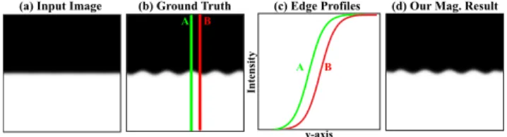
Figure 3: Synthetic Example: (a) The input image, a horizontal edge in the middle of the image carries a 0.1 pixel sinusoidal per-turbation,f (x) = 0.1 sin(2πωx). (b) Magnification of the ground truth perturbation by a factor of 20. (c) Two edge profiles obtained by sampling the intensity values in (b) along the green (A) and red (B) vertical lines, respectively. The edge profiles are related by 1D translation. (d), the small perturbation in the input (a) are revealed by our method.

it only reflects a constant shift in f (x), i.e., an overall translation of the object of interest. Moreover, for many applications, such global translation is filtered out by band-passing the deviation sig-nal. Therefore, for convenience, we treat this translated edge profile as the original edge profile S(y). In practice, to be more robust to outliers in the edge profiles, we use the median instead of the mean. With S(y) in hand, the deviation signal f (x) is then obtained by estimating the optimal 1D translation, in terms of least square error, between the S(y) and each of the observed ones. In the discrete domain, this takes the form of:

arg minX

y

(I(x, y) − S(y) − f (x)S0(y))2, (7) which leads to:

f (x) ≈ P y(I(x, y) − S(y))S 0 (y) P yS0(y)2 (8) As can be seen from the equation, pixels for which S0(y) = 0 do not contribute at all to the solution. Our formulation is similar to the seminal method [Lucas et al. 1981] used for image registration.

3.3 Canonical Stripe Representation

The region in the vicinity of each fitted shape is warped into a canonical stripe. This representation allows us to treat any type of fitted shape as a horizontal line. For an arbitrary geometric shape, let {~pi} be points sampled along it. The shape has a local normal direction at every point, which we denote by ~n(~pi). For each point, the image is sampled in the positive and negative normal direction ±n(~pi), using bicubic interpolation to produce the canonical stripe. This sampling is done at a half pixel resolution to prevent spatial aliasing (which may occur for high frequency diagonally oriented textures). To prevent image content far from the shape from affect-ing the deviation signal, we sample only a few pixels (3-5 pixels) from the shape. In the resulting stripe, the edge is now a horizontal line and the vertical axis is the local normal direction ~n(pi). In many cases, the image may be highly textured near the shape’s contour, which can invalidate our assumption of a constant edge profile (Eq. 2). To address this problem, we apply the matting al-gorithm of Levin et al. [2008] on the sampled image stripe. The output alpha matte has the same sub-pixel edge location as the real image, but removes variations due to texture and turns real image stripes into ones that more closely satisfy the constant edge profile assumption. This can be seen in Figure 2(2), where the similarity between the matted stripe and the synthetic image shown in Fig-ure 3 is much stronger than between the synthetic image and the canonical stripe.

(a) Input Image (b) W/o Anti-aliasing (c) W/ Anti-aliasing

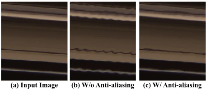
Figure 4: Deviations of Saturn’s rings amplified without and with the aliasing post-filter. Without it, there is a sinusoidal perturbation along the rings (b), but our post-filter reveals that it is actually just spatial aliasing in the input image (c). (Image courtesy of NASA.)

The input to the matting algorithm is the canonical stripe and an automatically generated mask, in which pixels on one side of the contour are marked as foreground and pixels on the other side as background. This mask provides the algorithm with a lot of infor-mation about where the edge is. This essential step substantially increases the signal to noise ratio and allows us to deal with chal-lenging, real world data as demonstrated in our experimental eval-uation (e.g., see Figure 5(d)).

The deviation signal is computed on the estimated alpha matte (as described in Sec. 3.2), and therefore represents the amount that the actual shape deviates from the ideal shape in the ideal shape’s local normal direction.

Spatial Anti-Aliasing For some images (e.g. astronomy), spa-tial aliasing in the input image can makes its way into the canon-ical stripe and then the deviation signal masquerading as a true signal. We address this problem by applying a dedicated spatial anti-aliasing post filter to remove these components. An example is shown in Figure 4, in which we used our method to amplify the deviations from all straight lines in a picture of Saturn’s rings. With-out the anti-aliasing filter, there is a sinusoidal deviation on all of the processed lines (Figure 4b). Our filter removes this artifactual deviation (Figure 4c).

Theoretically, spatial aliasing can occur at any frequency. How-ever, we can compute it as it depends on the edge’s orientation. Once computed, we filter out only that single frequency. The full derivation of our anti-aliasing filter is described in Appendix A. Note that our anti-aliasing filter may not have a significant impact on all images since reasonable camera prefilters often prevent alias-ing. However, we apply it as sanity check to lines in all images.

3.4 Synthesis

Now, that we have a filtered deviation signal for every fitted or user-chosen contour in the image, we seek to generate a new image, in which the objects carrying the deviations are warped, but other im-age content is not. We do this by first computing a 2D warping field, ~V (x, y) = {u(x, y), v(x, y)} that is constrained to match the amplified deviation signal at sampled locations along the contours. The flow field at the remaining pixels is determined by minimiz-ing an objective function that aims to propagate the field to nearby pixels of similar color, while setting the field to zero far from the contours.

By construction, the deviation signal is oriented in the normal di-rection to the contour at each point. At a pixel ~p := (x, y) sampled

along the sthcontour, we set the warping field to be equal to ~

V (~p) = αfs(~p)~ns(~p) (9) where α is an amplification factor, fs(~p) is the deviation signal of the sth contour at location ~p and ns(~p) is the local normal direction of the sth contour at ~p. Every pixel that touches a contour will in-troduce a hard constraint of this form. If a pixel is on two contours, we average the constraints.

The hard constraints on the warping field imposed by Eq. 9 give sparse information that must be propagated to the rest of the image. We follow the colorization method of Levin et al. [2004], and de-fine the following objective function for the horizontal component u (the same objective is defined for the vertical component)

arg min u X ~ p  (u(~p) − D(~p) X ~ q∈N (~p) w~p~qu(~q)   2 , (10)

where ~p and ~q are coordinates in the image, N (~p) is the eight-pixel neighborhood around ~p, w~p~q = exp−kI(~p)−I(~q)k

2_/2σ2 is a weighting function measuring the similarity of neighboring pixels and D(~p) is a weighting function that measures the distance from the point ~p to the nearest point on a contour (computed using the distance transform). The inner sum in the objective function is the average warping field of all pixels of similar color to ~p in its neigh-borhood. The term D(~p) shrinks at pixels far from contours. At pixels far from contours, D(~p) is close to zero and the summand becomes u(~p)2, which encourages the warping field to go to zero. Since the objective function is a least squares problem, it can be minimized by solving a sparse linear system.

Once the warping field is estimated, the rendered image is then given by inverse warping: bIdev= I(x + u, y + v).

3.5 User Interaction

While it is possible to perform our processing automatically, we give the user the ability to control which objects or contours are analyzed, what components of the deviation signal should be am-plified and what parts of the image should be warped.

A simple GUI is provided for users that want to pick specific objects to amplify. Because it is tedious to specify the exact location of a contour in the image, the user is only required to give a rough scribble of the object. Then, an automatic fitting algorithm is used to find the location of all elementary shapes in the object and we use the one that is closest to what the user scribbled [P˘atr˘aucean et al. 2012]. We show an example of a user selecting a line on top of a bookshelf in the supplementary material.

For a contour specified by points {~pi}, the raw deviation signal f (~pi) can contain signals that correspond to several different types of deviations. In addition, the DC component of the signal corre-sponds to an overall shift of the entire object and we may want to adjust or remove it. Noise may also be present in the deviation sig-nal. For these reasons, we apply bandpass filtering to the raw signal f (x). The user can specify the cutoffs of the filter depending on the application. In the sand dune example (Figure 2), we removed the very low and high frequencies to remove noise and the overall curvature of the dune. And in the house example (Figure 1), we only amplified the low frequencies, setting the DC to make the sure the deviation signal was zero at the endpoints, so they did not get warped. The user also specifies an amplification factor indicating the amount by which the deviations should be magnified.

For examples in which the fitted shapes are straight lines, we allow the user to specify a bounding box around the contour of interest

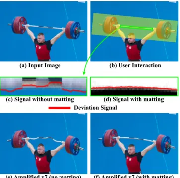
(e) Amplified x7 (no matting) (a) Input Image

(c) Signal without matting

(f) Amplified x7 (with matting) Deviation Signal

(d) Signal with matting (b) User Interaction

Figure 5: Revealing the bending of a weighted steel barbell and a comparison of our method with and without matting. An image stripe is taken from the input image (a) and the deviation signal is overlayed on the image stripe without matting (c) and with it (d). The deviations in the weightlifter’s barbell are amplified without matting (e) and with matting (f). (Image courtesy of Jay Smidt.)

(see Figure 5(b)) to ensure that everything within the bounding box gets warped according to the deviation signal. The diagonal of the bounding box is projected onto the fitted line. In the direction par-allel to the line, the deviation signal is extrapolated to the ends of the box using quadratic extrapolation of the points close to the end. For all other points in the bounding box, we modify the hard con-straints of the above objective function. Specifically, for each point ~

p in the bounding box, we find the nearest point on the contour ~q and set the warping field at ~p to be the same hard constraint as ~q. This ensures that all objects within the bounding box get warped in the same way.

4

Results

The results were generated using non-optimized MATLAB code on a machine with a quad-core processor with 16 GB of RAM. Our processing times depend on the number of shapes processed and the image’s resolution. It took twenty seconds to produce our slowest result, in which 180 lines were processed in a 960 × 540px image. In some examples, we corrected for lens distortion to prevent it from being interpreted as deviations from straight lines. This is done using the commercial software DxO Optics Pro 10 [DxO ], which automatically infers the lens type from the image’s metadata, and then undoes the distortion using this information.

We present our results on real images, and perform a qualitative and quantitative evaluation on both synthetic and real data.

Deviation Magnification in the World We applied our algorithm on natural images, most of which were taken from the Web. These images are of real world objects, which have highly textured edges making them challenging to process.

In Figure 1, we reveal the sagging of a house’s roof by amplifying the deviations from a straight line fitted to the upper part of the roof. To validate our results, we processed two different images of the house in which the roof is at different locations of the image (Figure 1(a,c)). As can be seen in Figure 1(b,d), the roof’s sagging remains consistent across the different views. Revealing this subtle sagging of a building’s roof is a useful indication of when it needs to be repaired. Because the house’s roof spans such a large part of the image, the effect of lens distortion may not be negligible. To avoid this problem, we used DxO Optics Pro 10 to correct for lens distortion.

In Figure 2, we reveal the periodic ripple pattern along the side of a sand dune by amplifying its deviations from a straight line by ten times. Here, even the intensity variations along the line show the deviations. The raw signal was bandpassed in order to visualize only the ripple marks and not the overall curvature of the dune. Knowing what these imperceptible ripple marks look like may have applications in geology [Nichols 2009].

In Figure 5, we reveal the bending in a steel barbell due to the weights placed on either end by amplifying the low frequencies of the deviation from a straight line. In addition to specifying the line segment to be analyzed, the user also specifies a region of in-terest, marked in green in Figure 5(b), specifying the part of the image to be warped. In this example, the necessity of matting in our method is demonstrated. Without matting, the color difference between the darker and lighter parts of the barbell causes a shift in the raw deviation signal (Figure 5(c)), which causes the barbell to appear wavy after amplification (Figure 5(e)). With matting, we are able to recover the overall curvature of the barbell and visualize it (Figure 5(d,f)).

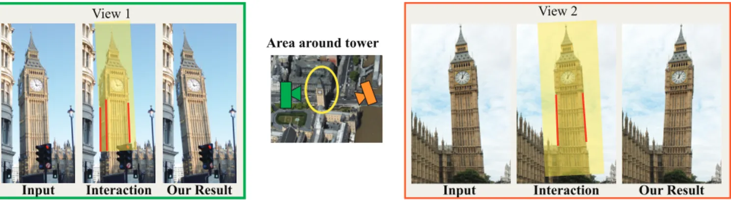
Civil engineers have reported that Elizabeth Tower (Big Ben) is leaning at an angle of 0.3 degrees from vertical [Grossman 2012]. Our algorithm reveals this visually in two independently processed images of the tower from different viewpoints (Figure 6). Here too, the consistency across views supports our results. In this example, instead of directly using the edges of the tower as the fitted geome-try, we use vertical lines going through the vanishing point. We find them by using a technique from Hartley and Zisserman [2003]. In order to amplify only the tilting of the tower (which corresponds to low frequencies in the deviation signal), while ignoring deviations due to bricks on the tower (high frequencies), we lowpass the de-viation signal. The filtered signal is then extrapolated to the entire user-specified bounding box to warp the entire tower. The size of the deviations for lines on the tower are on average 2-3x larger than the deviations of lines on other buildings indicating that we are ac-tually detecting the tilt of the tower. Visualizing the subtle tilt of buildings may give civil engineers a new tool for structural moni-toring. Lens distortion is corrected as a preprocessing step (see the supplementary video for our results w/o lens distortion).

Deviation Magnification in Videos In the following examples, we tested our method on several video sequences. Specifically, our method was applied to each of the frames independently, without using any temporal information. The fitted shapes in each frame were detected automatically. The temporal coherence of the ampli-fied structures, processed independently for each frame, validates our results. For some of the examples, we were also able to compare our results to motion magnification applied to stabilized versions of the sequences [Wadhwa et al. 2013]. Our results and comparisons on the entire sequences are included in the supplementary material. The video ball is a high speed video (13,000 FPS) of a lacrosse ball hitting a black table in front of a black background. The trajectory of the ball is illustrated in Figure 7, and two of the frames that correspond to the red and green locations of the ball are shown in Deviation Magnification: Revealing Departures from Ideal Geometries • 226:5

Input Interaction

View 1 View 2

Our Result Input Interaction Our Result

Area around tower

Figure 6: Elizabeth Tower (Big Ben) becomes the leaning tower of London. We process the two images of the tower independently. Parallel vertical lines in the input image are used to compute the vanishing point of the input images (only crops of which are shown here). In (b), the user specifies the lines that go through the vanishing point (marked in red) and a region of interest (marked in semi-transparent yellow). Our method computes the deviation from the fitted line, and synthesizes a new image, in which the deviation is exaggerated.

Input

Our

Result

time

(e) Ball Trajectory

0 0

(c) (d)

(f) Raw Deviation Signal

(a) (b)

Figure 7: Revealing the distortion and vibrations of a ball when it hits a table. (a-b) two frames from the input video that correspond to the red and green locations of the ball in (e), respectively. Our method computes the deviation of the ball from a perfect circle in each of the frames independently. (c-d), the rendering of (a) and (b), respectively, where the deviation is x10 larger. (e), the raw deviation signal, counterclockwise along the ball from0 to π.

Figure 7(a,b), respectively. We applied our framework to reveal the distortion in the shape of the ball, i.e., deviation from a perfect circle, when it hits the ground and travels upward from impact. Figure 7(c,d) shows our rendering of the two input frames where the deviation is ten times larger. Figure 7(f) shows the raw deviation signal for the moment of impact (green location) as a function of the angle. Because the raw deviation signal appears to have most of its signal in a low frequency sinusoid, we apply filtering to isolate it to remove noise. Our results on the entire sequence not only reveals the deformation of the ball at the moment it hits the ground, but also reveals the ball’s post-impact vibrations. For comparison, we apply motion magnification with and without stabilizing the input video. Without stabilization, motion magnification fails because the ball’s displacement from frame to frame is too large. With stabilization, the results are more reasonable, but the moment of impact is not as pronounced. This is because the motion signal has a temporal dis-continuity when the ball hits the surface that is not handled well by motion magnification. In contrast, deviation magnification handles

(a) Input (b) Magnified x20

Figure 8: Revealing the vibrations of a bubble from a single frame. An input frame of two bubbles (a) was used to produce our mag-nification result (b) in which the low frequency deviations of each bubble were amplified. The shapes were automatically detected. No temporal information was used.

this discontinuity, as each frame is processed independently. Bubblesis a high speed video (2,000 FPS) of soap bubbles moving to the right shortly after their generation (Figure 8(a-b)). Surface tension causes the bubbles to take a spherical shape. However, vi-brations of the bubble and gravity can cause the bubble’s shape to subtly change. In this sequence, we automatically detect the best fit circles for the two largest bubbles and amplify the deviations cor-responding to low frequencies independently in each frame. This allows us see both the changing dynamics of the bubble and a con-sistent change in the bubble’s appearance that may be due to gravity. For comparison, we applied motion magnification to a stabilized version of the sequence. We used the fitted circles to align the bubbles in time and then applied motion magnification (similar to [Elgharib et al. 2015]). The magnified bubbles were then embed-ded back in the input video at their original positions using linear blending at the edges. This careful processing can also reveals the changing shape of the bubbles, but it does not show the deviations from circular that do not change in time, such as the effect of gravity on the bubble.

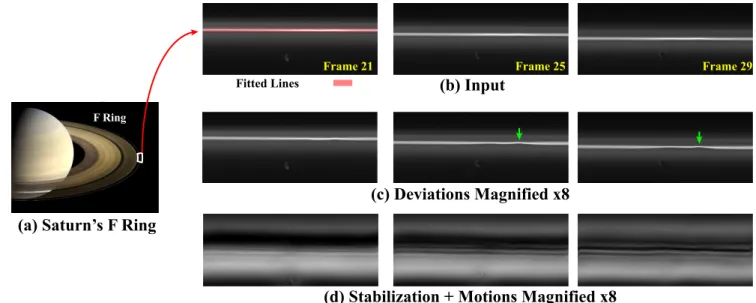
Figure 9(b) presents three frames from a 72 frame timelapse (cap-tured by the Cassini orbiter), showing Saturn’s moon Prometheus interacting with Saturn’s F ring. The frames were aligned by NASA such that the vertical axis is the distance from Saturn, which causes the rings to appear as horizontal lines. For every frame in the video, we amplified the deviations from the best-fit straight lines (marked in red in Figure 9(b)). This reveals a nearly invisible, temporally consistent ripple (Figure 9(c)). These kind of ripples are known to occur when moons of Saturn approach its rings [Sutton and

Kus-Frame 25 Frame 29

(b) Input

(d) Stabilization + Motions Magnified x8

Frame 21

(c) Deviations Magnified x8

F Ring

(a) Saturn’s F Ring

Figure 9: Deviation Magnification independently applied to each frame of a timelapse of Saturn’s moon interacting with its ring. Three frames from the timelapse (b) are processed using our new deviation magnification method (c) and using stabilization plus motion magnification (d). The lines used to do the stabilization and the fitting are shown in (b). The green arrows denotes the most salient feature after amplification. The full sequence is in the supplementary material. (Images courtesy of NASA.)

martsev 2013]. Applying our technique on such images may be use-ful for astronomers studying these complex interactions, and even might reveal new undiscovered gravitational influences in the rings. We also applied motion magnification to a stabilized version of the sequence. As can be seen in Figure 9(d), even with stabilization, magnifying changes over time produces a lot of unwanted artifacts due to temporal changes in the scene unrelated to the main ring. It is the spatial deviations from the model shape that are primarily interesting in this example rather than the changes in time. In candle, we use our method to reveal heated air generated by a candle flame from a single image (Figure 10(b-c)). To do so, we estimate the deviations from every straight line, automatically fit-ted to the background. As can be seen in Figure 10(b-c), the twenty times amplified image, and the warping field reveal the flow of the hot air. Visualizing such flow has applications in many fields, such as aeronautical engineering and ballistics. Other methods of recov-ering such flow such as background-oriented schlieren [Hargather and Settles 2010] and refractive wiggles [Xue et al. 2014], ana-lyze changes over time. While these methods are restricted to a static camera, our method is applied to every frame of the video independently and is able to reveal the heated air even when the camera freely moves. In addition, the bumps in the background are revealed as well. Note that spatially stabilizing such a sequence is prone to errors because the background is one-dimensional, the camera’s motions are complex and the candle and background are at different depths.

A similar result is shown in Figure 10(d-e) where a column of ris-ing smoke appears to be a straight line. By amplifyris-ing the devia-tions from straight, we reveal sinusoidal instabilities that occur in the smoke’s flow as it transitions from laminar to turbulent [Tritton 1988]. Here too, the processing is done on each frame indepen-dently.

Interactive Demo We have produced an interactive demo that can process a 200x150 pixel video at 5 frames per second (Fig-ure 11). The user roughly specifies the location of the line at the first frame, which is then automatically snapped to a contour. Our

(a) Input (b) Mag. x20 (c) Warping Field (d) Input

Candle

-0.2 px

0.2 px

(e) Mag. x3

Smoke

Figure 10: Revealing the distortions in a background of straight lines caused by heated air and sinusoidal instabilities of smoke flow in a single image. In candle, the deviation from every straight line is amplified twenty times. Both the amplified result and the overlayed vertical warping field are shown. In smoke, a single line is fitted to the input and the result is magnified three times.

demo is interactive because we only process a single shape. A video of this demo to show the buckling of a bookshelf under weight when the deviations from a straight line are amplified is provided in the supplementary materials.

4.1 Synthetic Evaluation

To evaluate the accuracy of our method in estimating the deviation signal, we tested it on a set of 7500 synthetic images. The images had known subtle geometric deviations, so that we could compare our result with the ground truth. The images were 200×200 pixels with a single edge (see Figure 12(a)). We varied the exact deviation, the orientation, the sharpness of the edge, the noise level and the texture on either side of the edge (Figure 12(a-b)). Specifically, ten different cubic spline functions with a maximum magnitude of 1 pixel were used as the deviation shapes. Ten orientations were sampled uniformly from 0◦to 45◦with an increment of 5◦. The edge profile was set to be a sigmoid function sigmf(δ,x) = 1/(1 + exp (−δx)) with δ = {0.5, 2, 5}).

We first performed an evaluation on images without texture. We Deviation Magnification: Revealing Departures from Ideal Geometries • 226:7

Figure 11: A frame from our interactive demo showing a bookshelf buckling under weight when deviations from a straight line are am-plified.

(e) Error: Half-Textured (f) Error: Fully-Textured

(a) Synthetic Image (b) Variations of Synthetic Images

Deviation (x10) Oriented Sharper Noisy Half-Textured Fully-Textured

(d) Error: Orientation and Sharpness (δ) (c) Error: Noise Level

Orientation (degree) δ=0.5 δ=2 δ=5 Err or (px) 0.10 0.05 0.00 _{0 15 30 45} Noise Level (px) Err or (px) 0.10 0.05 0.00 _{0 0.02 0.05 0.1} FT1 FT5 FT10 FT15 With Matting Without Matting Err or (px) 1.0 0.5 0.0 1.5 HT1 HT2 HT3 HT4 HT5 HT6 With Matting Without Matting Err or (px)0.2 0.1 0.0 0.3 0.4 Sample

Figure 12: Quantitative evaluation on synthetic data: (a), an ex-ample untextured image and its amplified version. (b), the data includes images with lines in different orientations, sharpness lev-els, noise levels and textures. (c), the error as a function of additive Gaussian noise. (d), the mean absolute error in the deviation sig-nal computed by our method, as a function of the orientation, for different sharpness levels. (e), the error w/ and w/o matting for half-textured images (shown below). (f), the error w/ and w/o matting for fully-textured images.

also tested the effect of sensor noise by adding white Gaussian noise with standard deviation σ = {0.02, 0.05, 0.1}. In Figure 12(c), we show the error of our algorithm, which grows only linearly with the noise-level even when it is 25 intensity levels (σ = 0.1).

In Figure 12(d), we present the mean absolute error between the estimated deviation signal and the ground truth as a function of the line orientation, for the three edge sharpness levels. The average error is very small at 0.03px, 3% of the maximum magnitude of the ground truth deviation signal (1 px). As expected, smoother edge profiles lead to smaller error due to less aliasing.

To quantify the effect of texture and the ability of matting to remove it, we tested our method on textured synthetic images. We used six different textures to perform experiments in which only one side of

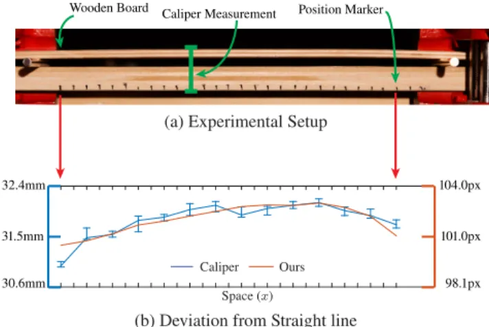
(a) Experimental Setup

(b) Deviation from Straight line Caliper Ours

Space (x)

Wooden Board _{Caliper Measurement} Position Marker

30.6mm 31.5mm 32.4mm 98.1px 101.0px 104.0px

Figure 13: Deviation from straight lines, controlled experiment. (a) The experimental setup, which is also the image used as an input to our framework. The measurements from digital calipers between the two wooden boards at each position marker and the deviation signal from our method are shown (b).

the edge was textured (Figure 12(e)). We also performed experi-ments in which both sides were textured using all 15 combinations of the six textures (Figure 12(f)). Figure 12(e-f) show the mean ab-solute error with and without matting for one-sided, half-textured images and two-sided, fully-textured images respectively. Without matting, the average error of our algorithm is about 0.3px for the half-textured examples and 1.5px for the fully-textured examples. With matting, the average errors shrink by ten times and are only 0.03px and 0.1px respectively. The highest errors are on a synthetic image, in which both sides of the image are of similar color. See the supplementary material for more details.

4.2 Controlled Experiments

We validated the accuracy of our method on real data by conducting two controlled experiments. In the first experiment, we physically measured the deviations from a straight line of a flexible wooden board. The board was affixed on top of two rods on a table using C-clamps (Figure 13). The base of the table served as the reference straight line. The distance from the bottom of the table to the top of the board was measured across a 29 cm stretch of it, in 2 cm increments using digital calipers (the markers in Figure 13(a)). The deviation signal from a straight line of the image of the wooden board is very similar to the caliper measurements (Figure 13(b)). In the second experiment, we affixed a stick onto a table and covered it with a sheet, with a pattern of ellipses on it (see Fig-ure 14(a)). The stick caused the sheet to slightly deform, which subtly changed the shape of some of the ellipses. To reveal the deformation, all the ellipses in the input image were automatically detected, and our method was applied to magnify the deviations of each ellipse from its fitted shape. A bandpass filter was applied to the deviation signal to remove overall translation due to slight errors in fitting and to smooth out noise. As can be seen in Figure 14(d)), only ellipses on or near the stick deform significantly, which reveals the stick’s unobserved location.

5

Discussion and Limitations

We have shown results on lines, circles and ellipses. However, ex-cept for the geometry fitting stage, our algorithm can generalize to arbitrary shapes. If a user can specify the location of a contour in an

image, our algorithm can be applied to it. For higher-order shapes such as splines, it can be unclear what should be a deviation and what should be part of the fitted model.

While we are able to reveal a wide variety of phenomena with our method, there are circumstances in which our algorithm may not perform well. If the colors on both sides of the shape’s contour are similar, we may not be able to compute its sub-pixel location. This is an inherent limitation in matting and edge localization. In some cases, changes in appearance along the contour may look like geometric deviations (e.g. a shadow on the object that is the color of the background). In this case, the deviation signal may have a few outliers in it, but otherwise be reliable.

Our method may also not be able to distinguish artifacts caused by a camera’s rolling shutter from a true geometric deviation in the world. If the camera or object of interest is moving, the camera’s rolling shutter could cause an artifactual deviation present in the image, but not in the world. Our method would pick this up and “re-veal” it. Bad imaging conditions such as low-light or fast-moving objects could cause a noisy image with motion blur, which would be difficult for our system to handle.

6

Conclusions

We have presented an algorithm, Deviation Magnification, to exag-gerate geometric imperfections in a single image. The algorithm involves three steps: model-fitting, deviation analysis, and visual exaggeration. Since the deviations from the geometric model may be very small, care is taken to account for pixel sampling, and image texture, each of which can otherwise overwhelm the small signal we seek to reveal.

Our method successfully reveals sagging, bending, stretching and flowing that would otherwise be hidden or barely visible in the in-put images. We validated the technique using both synthetically generated and ground-truth physical measurement and we believe that our method can be useful in many domains such as construction engineering and astronomy.

Our videos, results and supplementary material are available on

the project webpage: http://people.csail.mit.edu/

nwadhwa/deviation-magnification/.

7

Acknowledgments

We would like to thank the SIGGRAPH Asia reviewers for their comments. We acknowledge funding support from Shell Re-search, the Qatar Computing Research Institute, ONR MURI grant N00014-09-1-1051 and NSF grant CGV-1111415.

Appendix A: Derivation of Anti-aliasing Filter

We describe in more detail our anti-aliasing post-filtering step. To determine which frequencies correspond to aliasing, we perform the following frequency analysis on a continuous image of a straight line.

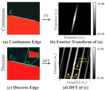
Let I(x, y) be a continuous image of a step edge of orientation θ (Figure 15(a)). If the edge profiles along the formed line L are con-stant, the 2D Fourier transform of the image F (ωx, ωy) is a straight line of orientation θ + π/2 in the frequency domain (Figure 15(b)). When the continuous scene radiance is sampled, a periodicity is in-duced in F (ωx, ωy). That is, the Fourier transform of the discrete

(a) Input (b) Source of Deformation

(c) Fitted Ellipses (automatically) (d) Magnification x7

Figure 14: Deviation from ellipses, controlled experiment. A sheet with ellipses on it is draped over a table with a stick on it (a-b). The deviation from every ellipse is automatically fitted (c) and then amplified by seven times (d) revealing the unobserved location of the stick. image ID(x, y) is equal to F (ID(x, y)) = ∞ X n=−∞ ∞ X m=−∞ F (ωx− nfs, ωy− mfs) (11) where fsis the spatial sampling rate of the camera. This periodicity creates replicas in the Fourier transform that may alias into spatial frequencies along the direction of the edge (Fig. 15(d)). Our goal is to derive the specific frequencies at which these replicas occur. Since the deviation signal is computed for the line L, we are only interested in aliasing that occurs along it. Thus, we derive the 1D Fourier transform of the intensities on the discrete line LDvia the sampled image’s Fourier transform F (ID(x, y)). Since F (ωx, ωy) is non-zero only along the line perpendicular to L, the discrete Fourier transform F (ID(x, y)) contains replicas of this line cen-tered at n(fs, 0) + m(0, fs) for integer n and m (from Eq. 11). Us-ing the slice-projection theorem, the 1D Fourier transform of LDis given by the projection of F (ID(x, y)), i,e, the image’s 2D Fourier transform, onto a line with orientation θ that passes through the ori-gin. This means that the replica’s project all of their energy onto a single point on LDat location

nfscos(θ) + mfssin(θ), (12)

which gives us the value of the aliasing frequencies along the image slices. The first and usually most dominant such frequency occurs when exactly one of n or m is equal to one and has value

fsmin(| cos(θ)|, | sin(θ)|). (13)

The exact strength and importance of each aliasing frequency de-pends on the edge profile. Since most real images are taken with cameras with optical anti-aliasing prefilters, they have softer edges. We found it sufficient to only remove the lowest aliasing frequency (Eq. 13) to mitigate the effects of aliasing. To handle small de-viations in orientation, we remove a range of frequencies near the aliasing frequency (Eq. 13).

(c) Discrete Edge -60 -50 -40 -30 -20 -10 0 10 20 30 Replicas Aliasing Frequency 30 dB -60 dB Frequency (ωx) Frequency ( ωy ) fs -fs -fs fs 0 0

(a) Continuous Edge (b) Fourier Transform of (a)

L

L

Continuous

Discrete

Figure 15: Causes of spatial aliasing and how to find the alias-ing frequency.‘ (a), a continuous edge and its discretization (c); (b,d), the Fourier transforms of (a,c) respectively. (d), replicas in the Fourier transform cause spatial aliasing along the lineL.

References

BLANZ, V.,ANDVETTER, T. 1999. A morphable model for the synthesis of 3d faces. In Proceedings of the 26th annual con-ference on Computer graphics and interactive techniques, ACM Press/Addison-Wesley Publishing Co., 187–194.

CANNY, J. 1986. A computational approach to edge detection. Pattern Analysis and Machine Intelligence, IEEE Transactions on, 6, 679–698.

DEKEL, T., MICHAELI, T., IRANI, M., ANDFREEMAN, W. T. 2015. Revealing and modifying non local variations in a sin-gle image. ACM Transactions on Graphics (TOG) special issue. Proc. SIGGRAPH Asia.

DOLLAR´ , P.,ANDZITNICK, C. L. 2013. Structured forests for fast edge detection. In Computer Vision (ICCV), 2013 IEEE In-ternational Conference on, IEEE, 1841–1848.

DOLLAR, P., TU, Z.,ANDBELONGIE, S. 2006. Supervised learn-ing of edges and object boundaries. In Computer Vision and Pattern Recognition, 2006 IEEE Computer Society Conference on, vol. 2, IEEE, 1964–1971.

DUDA, R. O.,ANDHART, P. E. 1972. Use of the hough transfor-mation to detect lines and curves in pictures. Communications of the ACM 15, 1, 11–15.

DxO OpticsPro 10. http://www.dxo.com/us/photography/photo-software/dxo-opticspro.

ELGHARIB, M., HEFEEDA, M., DURAND, F., ANDFREEMAN, W. T. 2015. Video magnification in presence of large motions. In Proceedings of the IEEE Conference on Computer Vision and Pattern Recognition, 4119–4127.

FISCHLER, M. A.,ANDBOLLES, R. C. 1981. Random sample consensus: a paradigm for model fitting with applications to im-age analysis and automated cartography. Communications of the ACM 24, 6, 381–395.

FREEMAN, W. T.,ANDADELSON, E. H. 1991. The design and use of steerable filters. IEEE Transactions on Pattern analysis and machine intelligence 13, 9, 891–906.

GROSSMAN, W. M. 2012. Time shift: Is london’s big ben falling down? Scientific American.

HARGATHER, M. J., AND SETTLES, G. S. 2010. Natural-background-oriented schlieren imaging. Experiments in fluids 48, 1, 59–68.

HARTLEY, R.,ANDZISSERMAN, A. 2003. Multiple view geome-try in computer vision. Cambridge university press.

LEVIN, A., LISCHINSKI, D.,ANDWEISS, Y. 2004. Colorization using optimization. 689–694.

LEVIN, A., LISCHINSKI, D.,ANDWEISS, Y. 2008. A closed-form solution to natural image matting. Pattern Analysis and Machine Intelligence, IEEE Transactions on 30, 2, 228–242. LIM, J. J., ZITNICK, C. L.,ANDDOLLAR´ , P. 2013. Sketch

to-kens: A learned mid-level representation for contour and object detection. In Computer Vision and Pattern Recognition (CVPR), 2013 IEEE Conference on, IEEE, 3158–3165.

LIU, C., TORRALBA, A., FREEMAN, W. T., DURAND, F.,AND

ADELSON, E. H. 2005. Motion magnification. In ACM Trans-actions on Graphics (TOG), vol. 24, ACM, 519–526.

LUCAS, B. D., KANADE, T., ET AL. 1981. An iterative image registration technique with an application to stereo vision. In IJCAI, vol. 81, 674–679.

NALWA, V. S.,ANDBINFORD, T. O. 1986. On detecting edges. Pattern Analysis and Machine Intelligence, IEEE Transactions on, 6, 699–714.

NICHOLS, G. 2009. Sedimentology and stratigraphy. John Wiley & Sons.

P ˘ATRAUCEAN˘ , V., GURDJOS, P.,ANDVONGIOI, R. G. 2012. A parameterless line segment and elliptical arc detector with enhanced ellipse fitting. In Computer Vision–ECCV 2012. Springer, 572–585.

SUTTON, P. J.,ANDKUSMARTSEV, F. V. 2013. Gravitational vor-tices and clump formation in saturn’s f ring during an encounter with prometheus. Scientific reports 3.

TRITTON, D. J. 1988. Physical fluid dynamics. Oxford, Clarendon Press, 1988, 536 p. 1.

WADHWA, N., RUBINSTEIN, M., DURAND, F., ANDFREEMAN, W. T. 2013. Phase-based video motion processing. ACM Trans-actions on Graphics (TOG) 32, 4, 80.

WADHWA, N., RUBINSTEIN, M., DURAND, F., ANDFREEMAN, W. T. 2014. Riesz pyramid for fast phase-based video mag-nification. In Computational Photography (ICCP), 2014 IEEE International Conference on. IEEE.

WU, H.-Y., RUBINSTEIN, M., SHIH, E., GUTTAG, J. V., DU

-RAND, F.,ANDFREEMAN, W. T. 2012. Eulerian video magni-fication for revealing subtle changes in the world. ACM Trans. Graph. 31, 4, 65.

XUE, T., RUBINSTEIN, M., WADHWA, N., LEVIN, A., DURAND, F., ANDFREEMAN, W. T. 2014. Refraction wiggles for mea-suring fluid depth and velocity from video. In Computer Vision– ECCV 2014. Springer, 767–782.