The two-way nested global chemistry-transport zoom model TM5: algorithm and applications

(1)

HAL Id: hal-00301349

https://hal.archives-ouvertes.fr/hal-00301349

Submitted on 28 Jul 2004

HAL is a multi-disciplinary open access

archive for the deposit and dissemination of sci-entific research documents, whether they are pub-lished or not. The documents may come from teaching and research institutions in France or abroad, or from public or private research centers.

L’archive ouverte pluridisciplinaire HAL, est destinée au dépôt et à la diffusion de documents scientifiques de niveau recherche, publiés ou non, émanant des établissements d’enseignement et de recherche français ou étrangers, des laboratoires publics ou privés.

The two-way nested global chemistry-transport zoom

model TM5: algorithm and applications

M. Krol, S. Houweling, B. Bregman, M. van den Broek, A. Segers, P. van

Velthoven, W. Peters, F. Dentener, P. Bergamaschi

To cite this version:

M. Krol, S. Houweling, B. Bregman, M. van den Broek, A. Segers, et al.. The two-way nested global chemistry-transport zoom model TM5: algorithm and applications. Atmospheric Chemistry and Physics Discussions, European Geosciences Union, 2004, 4 (4), pp.3975-4018. �hal-00301349�

(2)

ACPD

4, 3975–4018, 2004

TM5: a two-way nested zoom model

M. Krol et al. Title Page Abstract Introduction Conclusions References Tables Figures J I J I Back Close Full Screen / Esc

Print Version Interactive Discussion

Atmos. Chem. Phys. Discuss., 4, 3975–4018, 2004 www.atmos-chem-phys.org/acpd/4/3975/

SRef-ID: 1680-7375/acpd/2004-4-3975 © European Geosciences Union 2004

Atmospheric Chemistry and Physics Discussions

The two-way nested global

chemistry-transport zoom model TM5:

algorithm and applications

M. Krol1, S. Houweling2, B. Bregman3, M. van den Broek2, 3, A. Segers3, P. van Velthoven3, W. Peters4, F. Dentener5, and P. Bergamaschi5

1

Institute for Marine and Atmospheric Research Utrecht, The Netherlands

2

Space Research Organisation Netherlands, Utrecht, The Netherlands

3

Royal Netherlands Meteorological Institute, de Bilt, The Netherlands

4

National Oceanic and Atmospheric Administration, Climate Monitoring and Diagnostics Laboratory, Boulder, USA

5

Joint Research Centre, Institute for Environment and Sustainability, Ispra, Italy Received: 6 April 2004 – Accepted: 10 May 2004 – Published: 28 July 2004 Correspondence to: M. Krol (krol@phys.uu.nl)

(3)

ACPD

4, 3975–4018, 2004

Abstract

This paper describes the global chemistry Transport Model, version 5 (TM5) which al-lows two-way nested zooming. The model is used for global studies which require high resolution regionally but can work on a coarser resolution globally. The zoom algorithm introduces refinement in both space and time in some predefined regions. Boundary 5

conditions of the zoom region are provided by a coarser parent grid and the results of the zoom area are communicated back to the parent. A case study using 222Rn measurements that were taken during the MINOS campaign reveals the advantages of local zooming. As a next step, it is investigated to what extent simulated concentrations over Europe are influenced by using an additional zoom domain over North America. 10

An artificial ozone-like tracer is introduced with a lifetime of twenty days and simplified non-linear chemistry. The concentration differences at Mace Head (Ireland) are gen-erally smaller than 10%, much smaller than the effects of the resolution enhancement over Europe. Thus, coarsening of resolution at some distance of a sampling station seems allowed. However, it is also noted that the budgets of the tracers change con-15

siderably due to resolution dependencies of, for instance, vertical transport. Due to the two-way nested algorithm, TM5 therefore offers a consistent tool to study the effects of grid refinement on global atmospheric chemistry issues like intercontinental transport of air pollution.

1. Introduction

20

In studies of the chemical composition of the atmosphere, measurements play a crucial role. Measurements of the atmospheric composition are conducted at surface stations, with balloon soundings, by aircraft sampling, and by means of satellite measurements. These measurements are often combined during intensive field campaigns, e.g. MI-NOS (Lelieveld et al.,2002a), TRACE-P (Jacob et al.,2003), in which the composition 25

(4)

con-ACPD

4, 3975–4018, 2004

ducted during longer time periods with the aim to study the long term changes and variability of the chemical composition of the atmosphere (Logan, 1999; Prinn et al.,

2000;Dlugokencky et al.,2003;Novelli et al.,2003).

In order to model the regional atmospheric composition it is often necessary to con-sider the entire Earth atmosphere in a model. For instance, the variability and long term 5

change in the methane concentration is governed not only by local sources, but also by (long range) transport, exchange with the stratosphere, and the chemical breakdown which occurs mainly in the tropics. Apart from the necessity to consider the global atmosphere, the interpretation of measurements requires simulations at a high spa-tial and temporal resolution. Only very remote measurements may be representative 10

for a large spatial domain, but most measurement sites are influenced by the local conditions. Spatial variability of emissions and other surface processes also call for a high spatial resolution. High resolution is also required for impact studies which have the aim to investigate the effects of air quality on human health or ecosystems. Cam-paigns, moreover, often focus on specific regions where both long range transport and 15

local or regional sources are important. Studies of intercontinental transport of pollu-tion (Wild and Akimoto,2001;Stohl et al.,2002;Wenig et al.,2003;Trickl et al.,2003;

Wang et al.,2003) and exchange of trace gases between the hemispheres require a hemispheric or global model domain. The same holds for inverse modeling studies of CO₂, CH₄, and CO (Kaminski et al.,1999;Houweling et al.,1999;Bergamaschi et al., 20

2000;Bousquet et al.,2000;R ¨odenbeck et al.,2003) where high resolution is required to reduce modeling and representation errors.

Computationally it is not possible to model the atmospheric composition both at the global scale and at a high resolution. One might ask, however, whether it is neces-sary to resolve the chemical composition of the South Pole at high resolution when 25

the region of interest lies on the northern hemisphere. A possibility to zoom in over a specific region is advantageous, at least from a computational point of view. The general concept of zooming is that the global chemical composition is modeled at a relatively coarse resolution that represents the main transport features. This

(5)

compo-ACPD

4, 3975–4018, 2004

sition then serves as a boundary condition for a regional simulation. This so-called one-way nested approach can be made two-way by feeding the calculated composi-tion of the zoom region back into the global domain. As an alternative to the use of zoom regions as described here, stretched grids have been employed to locally refine the model resolution (e.g.Cosme et al.,2002).

5

Recently, several atmospheric chemistry studies have employed grid-nesting. How-ever, most of these studies are regional and do not consider a global domain. For instance, the Regional Atmospheric Modelling System (RAMS) (Cotton et al.,2003) has been used to simulate the chemical composition over the south of France (Taghavi

et al.,2003). This study focusses on regional scales but employs a similar two-way 10

nested approach as used in TM5. The MM5 model has been coupled with a chemistry module and a region south of the Alps was studied in detail (Grell et al., 2000). In other studies (Soulhac et al.,2003;Tang,2002) a chain of models is used with a one-way nested information stream from the coarse to the finer scales. The regional high resolution air pollution model (REGINA) simulates the northern hemisphere at a rela-15

tively coarse resolution and employs one-way nesting to zoom in over Europe (Frohn

et al.,2003). One way nesting was also employed byJonson et al.(2001) who coupled the global Oslo CTM2 model to the regional Eulerian Photochemistry Model (EMEP). The focus of that study was on intercontinental transport and it was concluded that air pollution episodes in Europe are largely determined by emissions within the Euro-20

pean domain. Somewhat contradictory results were found by Bauer and Langmann

(2002) and Langmann et al.(2003) who used a global to mesoscale one-way nested model chain to simulate atmospheric ozone chemistry. They found that regional scale chemistry simulations improve when lateral boundary conditions from a global model simulation are used. Also, a significant contribution of long range transport to a pol-25

lution event over Europe was found. Nevertheless, a common conclusion of all these studies is that the comparison with observations normally improves with resolution. A large part of this improvement is due to better resolved emissions, especially near urban areas (Tang,2002).

(6)

ACPD

4, 3975–4018, 2004

This paper describes the numerical approach of a two-way nested global zoom model, named Tracer Model, version 5 (TM5). The main innovative feature of TM5 is the possibility to use two-way nesting along with a consequent use of the same chemi-cal and physichemi-cal parameterisations at different model resolutions. While some technical details as well as some first applications of the TM5 model have been described in ear-5

lier publications (Berkvens et al., 1999; Krol et al., 2002, 2003; Broek et al., 2003), we want to present here a comprehensive description of the TM5 model. Since TM5 is an off-line model (depending on meteorological data calculated by a weather fore-cast or climate model), we also discuss in some detail the pre-processing system that has been developed for the meteorological data that are needed to run the model. In 10

order to evaluate the transport of the model, we present some new results that have been obtained with TM5. To highlight the effects of a refinement in resolution on the model results, we focus on measurements made at Crete (Greece) during the MINOS campaign in August 2001 (Lelieveld et al., 2002a). The TM5 model is designed for global studies of atmospheric chemistry, such as intercontinental and interhemispheric 15

exchange and the effects of grid refinement on the budgets of chemically active com-pounds. To highlight these issues without yet introducing full atmospheric chemistry, we present an artificial tracer study in Sect.3.2. Finally we discuss future plans and ongoing developments.

2. Model description

20

2.1. Historical perspective

TM5 is named after the parent TM3 model and uses many of the concepts and param-eterisations that were present in that model. The TM model was originally developed byHeimann et al.(1988) and has been widely used in many global atmospheric chem-istry studies. Examples of such studies include the impact of higher hydrocarbons on 25

(7)

ACPD

4, 3975–4018, 2004

a 1978–1993 model simulation (Dentener et al.,2003), a comparison between mod-eled ozone columns and satellite observations (Peters et al.,2002) and the stability of hydroxyl radical chemistry (Lelieveld et al.,2002b).

2.2. Two-way nested zoom algorithm

Like in the TM3 model, the transport, emissions, deposition and chemistry of tracers is 5

solved by means of operator splitting. This approach has the important advantage that small time steps due to the stiff chemistry and vertical mixing operators can be avoided by applying tailored implicit schemes (Verwer et al., 1999). Both TM3 and TM5 are off-line models in which the meteorological data are provided by the model of the Euro-pean Centre for Medium Range Weather Forecast (ECMWF). Basic requirements that 10

we impose on the zooming algorithm are mass conservation and positiveness. Neg-ative concentrations should be avoided since these cause problems in mathematical routines that solve the system of equations of the chemical interactions between the species. The mathematical foundations of the mass-conserving transport within the zoom algorithm were presented byBerkvens et al.(1999). The implementation of this 15

algorithm and the coupling with emission, deposition, convection, and chemistry was described byKrol et al. (2002). Here, we summarize only the essential points of the algorithm and refer to the original work for more details.

The central idea behind the nesting technique is that over some selected regions the Chemistry Transport Model (CTM) is run simultaneously at various resolutions. The 20

coarsest region represents the global domain and provides the boundary conditions for one or more nested regions. Within a nested region one or more, still finer resolved regions can be nested. Given the desired model set-up, a tree is built where for each region the parent and the children are defined. A region can act both as a parent and as a child. A parent provides the boundary conditions for its children and the children are 25

used to update the information of the parent, which makes the nesting algorithm two-way. Figure1presents an example of a grid definition that has been defined to study the European area. Globally, a horizontal resolution of 6◦×4◦ (longitude×latitude) is

(8)

ACPD

4, 3975–4018, 2004

employed. The European domain is resolved at a resolution of 1◦×1◦. In order to allow a smooth transition between these two regions, a European domain with a resolution of 3◦×2◦ has been added. This latter domain is the child of the global domain and the parent of the 1◦×1◦model area. For mass conservation it is important that the regions share a common boundary.

5

Although is was shown that zooming in the vertical direction is possible when only advection processes are considered (Berkvens et al.,1999), this possibility is not in-cluded because the coupling with the convection would cause severe technical prob-lems. Therefore, all regions share the same vertical layer structure. The layers in the TM5 model are compatible with the hybrid sigma-pressure coordinate system that is 10

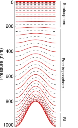
employed by the ECMWF model. Thus, either the ECMWF layers are used, or some layers are combined to a coarser resolution. The current operational ECMWF model version employs 60 layers, which have been transformed into 25 model layers for the European model set-up (see Fig.2). Since the focus of this model version is mainly on the troposphere, higher vertical resolution is maintained in the boundary layer and 15

in the free troposphere. Another implementation of the TM5 model focuses on the stratosphere (Broek et al.,2003) and retains more vertical layers above 200 hPa.

The nesting algorithm is designed for use in combination with operator splitting. The general steps that are considered in the model are advection in the X, Y, and Z direc-tions, parameterisation of sub-grid scale mixing by deep convection and vertical di ffu-20

sion (V), and chemistry (C). The latter process may include the emission and wet and dry deposition of chemical species. The operator splitting as applied in the three-region European-focused TM5 version is given in Table1. The refinement in time relative to the global domain is 2 and 4 for regions 2 and 3, respectively. All model time steps are determined from a general time step∆T (normally 5400 s). In the global 6◦×4◦domain 25

all numerical time steps are∆T/2. This time step is ∆T/4 and ∆T/8 at resolutions of 3◦×2◦and 1◦×1◦, respectively. Most meteorological information is supplied on time in-tervals of 6 h, while meteorological information pertaining to boundary layer mixing and surface processes are provided every 3 h (see Appendix for a table that lists the TM5

(9)

ACPD

4, 3975–4018, 2004

input fields). These time intervals impose an upper limit to the model time step∆T. The upper part of Table1represents the steps that are taken in the time interval [t, t+∆T/2]. The second part of the table corresponds to the interval [t+∆T/2, t+∆T].

If only region 1 would be considered, the model would be similar to the previous TM3 model. Numerical studies have shown that the symmetrical operator splitting as applied 5

here produces more accurate results (Strang,1968;Berkvens et al.,2002). However, this symmetrical splitting can not always be preserved in the zooming algorithm. For instance, the (symmetrical) stepping order in region 1 reads XYZVCCVZYX while the order in region 2 (XYZVCCVZYXCVZYXXYZVC) is only partly symmetrical. When communication between the parent and children occurs, this is indicated by the arrows 10

in Table 1. Parents write the boundary conditions to their children (↓) whereas the parents are updated with the information calculated by their children (↑). An update of a parent involves a procedure in which the tracer masses of the parent are overwritten by information from the child cells. Likewise, boundary conditions (↓) are provided by overwriting some child cells with tracer masses from the parent. Note that the algorithm 15

allows for overlapping zoom regions, but that the results of the “last reporting” child will determine the status of the parent in the overlap zone of the children.

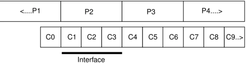
The mass-conserving advection algorithm that is used in the communication be-tween parent and children has been discussed in detail byBerkvens et al.(1999). In one dimension, the interface region is depicted in Fig.3. The corresponding algorithm 20

is summarized in Table2. Cell C0 is used to store the boundary condition that is pro-vided by the parent. The interface cells (C1, C2, and C3 in Fig.3) are crucial in the algorithm. The sum of the masses in the interface cells corresponds to the mass of a parent cell and the individual cells are of child resolution. The situation appears rela-tively straightforward in one dimension, but complications arise when the y-dimension 25

is also considered (denoted by the “...” in Table2). First, the boundary conditions that are written to the child may already have been advected by the parent. For instance, the tracer masses that are written to the child just before Y advection in the ↓X↓Y se-quence are already advected by the parent in the X direction. Therefore, the Y interface

(10)

ACPD

4, 3975–4018, 2004

cells of the child should not be advected again in the X direction. This is accomplished by restricting the X advection operator of the child to the core zoom region (from C4 on in Fig.3). Second, the interface cells should operate as “parent”-like cells in one direction (e.g. X), while they should act as “child”-like cells in another advection direc-tion (e.g. Y). In the algorithm, this is solved by “compression” of the grid in the direcdirec-tion 5

of the advection (cells C1, C2, and C3 are treated as one grid cell). After advection in that direction, the corresponding “decompression” is applied. Moreover, after each advection step the interface cells are mixed in order to avoid negative tracer masses (C1, C2, C3 receive equal masses).

Interface cells are partially advected during some stages of the algorithm (e.g. during 10

phase 5 of the algorithmic sequence in Table2). It was noted (Krol et al.,2002) that it should be avoided to perform processes like chemistry (C) and vertical mixing (V) on these partially advected interface cells. For that reason these operations on the interface cells are performed by the parent. Thus, the operations V and C are restricted to the core of the zoom region (from C4 on). In the algorithm, the parent is forced to 15

skip only the core cells of the child region in processing the V and C steps. After a child finishes an operator sequence, the parent cells are overwritten by the child cells in an update parent procedure (↑).

2.3. Tracer transport routines

The zooming algorithm has been coupled to the slopes advection scheme (Russel and

20

Lerner,1981). Apart from this algorithm, the second moments scheme (Prather,1986) has been implemented for numerical studies of stratospheric transport. Due to the regular latitude longitude grid in TM5, the x-spacing of the grid becomes very small close to the poles. In order to avoid violations of the Courant-Friedrichs-Lewy (CFL) criterion in these regions, two algorithmic provisions have been included. First, it is 25

possible to choose a reduced grid around the poles in the x-direction (Petersen et al.,

1998). During advection in the x-direction, several grid cells are combined in the longi-tudinal direction and the advection is performed on this coarser grid. After advection,

(11)

ACPD

4, 3975–4018, 2004

the masses of the coarse grid-cells are redistributed and the other processes are per-formed on the fine grid. The second provision consists of a general iteration in all advection routines. Whenever a CFL criterion is violated, the time step is reduced and the same advection routine is called two (and possibly more) times.

Non resolved transport by deep and shallow cumulus convection has been parame-5

terised according toTiedtke(1989). The vertical diffusion parameterisation ofHoltslag

and Moeng (1991) is used for near surface mixing. In the free troposphere, the formula-tion ofLouis(1979) is used. To remain consistent to the meteorological input fields that are used in the model, it is important to note that these parameterisations are similar to those that are employed by the ECMWF model.

10

One of the advantages of TM5 is that the same model is used at different resolutions. Therefore, it is considered crucial that the required meteorological data are consistent for the various model resolutions. Thus, the changes in the surface pressure should match the vertically integrated convergence of the mass fluxes, also within the zoom regions. As described in Sect.2.4, meteorological pre-processing software has been 15

developed to supply fully consistent meteorology at the different model resolutions. In an intercomparison exercise of 222Rn simulations with different models it was shown that the TM3 model did not capture the full diurnal cycle of near surface mixing (Dentener et al.,1999). It was analysed that 6-h input of ECMWF was not always suf-ficient to describe the development of the convective boundary layer over continents. 20

This layer remained systematically too shallow and it was concluded that the surface fields of latent and sensible heat fluxes should be resolved at a higher temporal resolu-tion. As a result, too much222Rn accumulation in the surface layer over the continents was observed. In order to solve this problem, the new pprocessing scheme re-trieves 3-h ECMWF surface fields on a 1◦×1◦ horizontal resolution. The calculation of 25

the diffusion coefficients in the boundary layer (Holtslag and Moeng,1991) requires in-tegration of these surface fields over the resolution of the region (e.g. on 6◦×4◦). These integrated fields are subsequently combined with the 6-h 3-D fields of wind shear, tem-perature and humidity. These latter fields remain on a 6-h resolution to reduce data

(12)

ACPD

4, 3975–4018, 2004

storage requirements.

Surface fields also include emissions, and parameters that are relevant for deposition of trace components. Similar to the heat fluxes, these fields are stored at a resolution of 1◦×1◦and, for the varying meteorological fields, on a 3-h basis (see table in Appendix). Prior to use in TM5, these fields are coarsened depending on the specific model set-up. 5

2.4. Meteorological pre-processing

The meteorological input for TM5 is created out of ECMWF data during a pre-processing stage. A complete list of TM5 input fields that are generated from ECMWF archived data is given in the Appendix. During the pre-processing stage, meteorologi-cal fields are converted from ECMWF resolution to the TM5 grid. Horizontally, the input 10

data is retrieved from the ECMWF archive at spectral resolution T159 or reduced Gaus-sian grid N80, which is equivalent to a resolution of about 1.125◦. Vertically, the data is retrieved at the 60 hybrid sigma-pressure levels employed by the ECMWF operational model.

Although interpolation from one resolution to the other is in general straightforward, 15

some topics will be discussed here in more detail: (i) the creation of mass fluxes, (ii) production of data for different zooming grids.

With TM5 being an Eulerian grid box model, the input required for advection should consist of mass fluxes through the boundaries of each grid box cell. The procedure is described in detail inSegers et al.(2002); here a brief outline is given.

20

The produced mass fluxes are valid for time intervals of 6 h. The vertical mass distributions (kg air) at the begin and end of an interval are computed from the surface pressures and the hybrid coefficients of the vertical layer structure. By this, the mass change per model grid cell (kg/s) during the time interval is defined. The mass fluxes (kg/s) through the boundaries should describe how air mass is flowing from grid box 25

to grid box, explaining the mass changes that are dictated by the changes in surface pressure. First, the vertical fluxes through the bottom of the grid boxes are computed by integration of horizontal divergence, and taking into account the horizontal pressure

(13)

ACPD

4, 3975–4018, 2004

gradients on the hybrid grid (Segers et al.,2002). Second, a first guess of the horizontal fluxes is computed from horizontal winds, which in turn are computed from the ECMWF divergence and vorticity. Finally, these first guess values are slightly modified in a way that the modified horizontal fluxes and the vertical fluxes together explain the observed mass gradient. Several tests have revealed that this new pre-processing algorithm 5

significantly improves the vertical transport in the tropopause region (Bregman et al.,

2001,2003).

To be able to run TM5 on various resolutions and for various zoom definitions, the meteorological input on different resolutions should be in agreement with one another. For example, the total air mass in a 3×2 block of 1◦×1◦cells should be equal to the the 10

mass in the 3◦×2◦cell by which it is covered.

To achieve this, an archive has been created with meteorological data on 3◦×2◦×60 resolution for 3-D fields such as mass fluxes, temperature, and humidity. This set is used as reference for meteorological fields on other horizontal or vertical resolutions. For a TM5 simulation with 3-level zooming such as depicted in Fig. 1, the input is 15

created in the following way:

– For the global 6◦×4◦ grid, the fields from the 3◦×2◦ archive are horizontally aver-aged, either area weighted or mass weighted. Mass fluxes through the bound-aries of the boxes are simply summed.

– 3◦×2◦ fields are just a subset from the archived fields. 20

– For 1◦×1◦ fields, the meteorological fields are extracted from the raw ECMWF data, in a similar way as has been done for the 3◦×2◦ archive. However, the errors associated with sampling the ECMWF fields depend on the resolution. In order to obtain 1◦×1◦ fields that are consistent with the 3◦×2◦ archived fields, the 1◦×1◦fields are slightly modified, such that totals (mass fluxes) or averages (other 25

fields) over blocks of 3×2 cells are equal to the values in the 3◦×2◦ archive. The modifications that are needed are generally very small.

(14)

ACPD

4, 3975–4018, 2004

The final step in production of the meteorological data is a reduction of the number of levels, if the model is defined on a subset of the full 60 vertical levels. Layers are combined by averaging or summing the meteorological parameters. When appropriate, weighting by the grid box masses is employed.

Creation of the 3◦×2◦×60 archive is the most expensive step in the procedure, since 5

this requires global evaluation and interpolation of the ECMWF data. However, once this set is available, the production of data for any set of zooming area’s and/or ver-tical levels is rather fast, since no interpolation is required (6◦×4◦ and 3◦×2◦ grids). Processing of the 1◦×1◦regions is only required for relatively small domains.

2.5. Implementation 10

The entire TM5 program has been coded in Fortran 90, which allows a flexible data structure. The model has been implemented and tested on various platforms, includ-ing some massive parallel machines. The operational version allows the use of multi processors employing the message parsing interface (MPI).

3. Case studies

15

3.1. 222Rn measurements on Crete

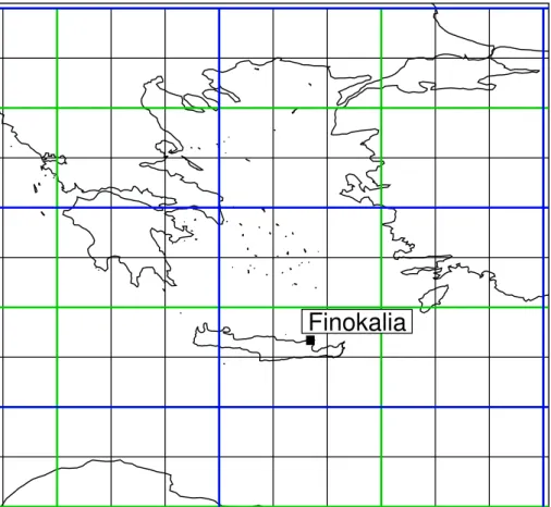
As mentioned in the introduction, the TM5 model setup is ideally suited for measure-ment campaigns. As an exploratory example, we will analyze the222Rn measurements that were made at the Finokalia station (Latitude 35◦190N, Longitude: 25◦400E) during the MINOS campaign (Lelieveld et al.,2002a). Figure 4shows the position of the Fi-20

nokalia measurement station, which is located on the island Crete in the Mediterranean sea. The station is positioned directly at the coast at an altitude of 130 m above sea level. During August 2001, the dominant wind direction is from north-westerly direc-tions and local emissions from Crete can generally be ignored (Mihalopoulos et al.,

1997;Kouvarakis et al.,2000). 25

(15)

ACPD

4, 3975–4018, 2004

Figure 4 depicts the model grid of TM5 at horizontal resolutions of 1◦×1◦, 3◦×2◦, and 6◦×4◦. On the coarsest resolution, the Finokalia station resides in the same grid-box as the southern part of Turkey. This implies that in the model simulation with only the coarsest resolution active (i.e. no zoom regions), the 222Rn emissions from Turkey (emissions are assumed to be 1.18 and 0.005 molecules cm−2s−1 over land 5

and sea, respectively (Dentener et al.,1999)) are sampled directly by the station in the model. On 3◦×2◦ the situation improves, but still considerable artificial spread of the 222

Rn emissions will occur. The 1◦×1◦horizontal resolution starts to resolve the actual distribution of the land masses, although it is clear that an even higher resolution would be desirable.

10

We sample the station concentration in our model by three methods. A large spread among the station concentrations calculated with these three methods signals large gradients and hence a large sampling error. The first sampling method simply takes the average mixing ratio of a tracer in the grid box. The second method employs the simulated values of the x, y, and z-slopes (Russel and Lerner, 1981) together with 15

the mean mixing ratio to interpolate to the station location, when this location is not in the center of the grid. The third method uses bilinear interpolation with the adjacent grid-cells in the x, y, and z directions. In this method, the value of the tracer slopes within a grid cell are not used. For the simulation on 6◦×4◦, large sampling errors are encountered (often >20%, not shown). The situation improves if the zoom regions 20

are activated. In the 1◦×1◦ simulation, difference in the sampling methods only arise if large concentration gradients are present close to the station (e.g. around 21 August, as discussed below).

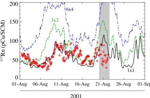
In Fig. 5 the222Rn concentrations simulated during August 2001 are compared to the measurements. A spin-up time of one month was used and bilinear interpolation 25

was employed to calculate the concentration at the location of Finokalia. The simulated station concentrations with only the global 6◦×4◦ resolution active, are systematically too high due to the emissions from the land masses that reside in the same grid box as the sampling station. The situation improves when the 3◦×2◦ European zoom domain

(16)

ACPD

4, 3975–4018, 2004

is used and an even better agreement is obtained when also the 1◦×1◦zoom region is used. Obviously, the match between measurements and model is still not perfect, but this example shows that the model results can improve considerably with higher model resolution.

The largest deviations between the 1◦×1◦simulation and the measurements are ob-5

served around 21 August (see grey bar in Figs.5–7), when the model overestimates the 222

Rn concentration by more than 50 pCu/SCM. In Fig.6the simulated concentrations are shown (in blue) for a location 1◦north of Finokalia. While for most of the simulation period the differences are small, it can be observed that the simulated concentrations around 21 August at open sea are drastically lower. To analyse the situation in more 10

detail, Fig. 7 shows the measured wind speed and direction along with the ECMWF values that are employed by the TM5 model. These values have been interpolated from the mass fluxes at the borders of the grid boxes. In order to exclude the influ-ence of the island of Crete on these interpolated values, the wind data have also been analysed at a position one degree north of Finokalia. At this northerly position the 15

measured wind speed is well reproduced by the mass fluxes derived from the ECMWF data. Not surprisingly given the location of the station, the measured wind speed at Finokalia appears to be representative for open sea. The measured wind direction is systematically more westerly than the wind direction in the model. This is most likely caused by local effects. At the coast, the airflow is forced upward or sideward, which 20

resulted in a backing of the wind direction. From the wind measurements and sim-ulations, the situation around 21 August stands out as a period of low wind speeds (gray bar). During such a period, the influence of Cretean emissions on the simulated 222

Rn concentration increases. The 222Rn accumulation is reinforced by the shallow boundary layer heights that are calculated during this period (see Fig.7). Since over 25

sea most of the solar heat flux generates evaporation, the depth of the boundary layer is predominantly determined by the vertical wind shear. Inspection of the lower panel in Fig.7 reveals that around 21 August, the boundary layer height collapses to about 100 m due to the low wind speeds. The grid box in which Finokalia resides contains

(17)

ACPD

4, 3975–4018, 2004

about 30% land masses, and a diurnal cycle in the calculated boundary layer height can be observed. Nevertheless, the boundary layer calculated by the TM5 model (and also by the ECMWF model) are very shallow. Inspection of the potential temperature profiles that were measured during the MINOS aircraft flights reveals a stable profile with several stronger inversions. One inversion layer is normally located between a few 5

hundred and 1000 m. Other inversions are found higher up, normally between 1 and 3 km, but the situation appears quite variable. In general it can be stated that vertical mixing is not very strong due to a stable temperature profile that is associated with subsiding air motions.

From the analysis presented here, it appears that measurements of wind data and 10

other meteorological parameters, including boundary layer heights, are (potentially) very important in the validation of the model results. Unfortunately, these meteoro-logical parameters are not always measured during field campaigns and at long term measurement stations.

3.2. Effects of zooming on the transport of chemical trace species 15

As noted in the previous section, pronounced improvements can be achieved by re-solving the interaction between emissions and transport of222Rn at a higher horizontal resolution. The artificial spread of local emissions is reduced and grid-boxes become more representative of the actual situation at sampling stations. Thus, the advan-tages of the local higher resolution are clear. Now, the question arises what the ef-20

fects are of using a coarse grid outside the zoom region. Related to this: why would a one-way nested zooming algorithm not be sufficient? To explore these questions we introduced some artificial tracers in TM5. These tracers mimic some features of tropospheric ozone chemistry, however, without the detailed chemical feedback mech-anisms. Tracer L1 (“NO_x”) and L20 (“CO”) are emitted using an emission distribution 25

and strength comparable of that of NO_x as given by the EDGAR3.2 inventory (Olivier

and Berdowski, 2001). To mimic the chemical breakdown of NO_x and CO, a simple radioactive decay (with lifetimes of 1 and 20 days, respectively) has been applied to

(18)

ACPD

4, 3975–4018, 2004

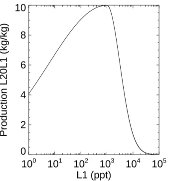
the tracers L1 and L20. Furthermore, an artificial tracer L20L1 (“O₃”) is introduced that is, like O₃, not emitted, but only chemically produced. The production of L20L1 is coupled to the decay of tracer L1 and this production depends non-linearly on the L1 concentration. Figure8depicts the assumed L20L1 production efficiency as a function of the L1 concentration. The curve consists of two linked Gaussian curves which are 5 given by: L1 > 1000 ppt : 10 exp −(log(L1)−3) 2 0.5 (1) L1 ≤ 1000 ppt : 10 exp −(log(L1)−3) 2 10.0 . (2)

At L1 concentrations of about 1000 ppt, the L20L1 production is assumed to be the most efficient (10 molecules L20L1 per lost L1 molecule). At lower and higher L1 con-10

centrations, the L20L1 production levels off, an effect that is stronger towards higher L1 concentrations. In this way, the resolution effects on the L1 concentrations are non-linearly translated into L20L1 production rates and concentrations. The lifetime of L20L1 has been taken as 20 days. As mentioned above, the L20L1 production curve can be interpreted as representative for NO_x dependent ozone production in the at-15

mosphere. More rigorous attempts to study the resolution dependence of atmospheric chemistry are outside the scope of this paper. The L20L1 tracer is merely used to study mechanisms that lead to differences in simulations with non-linear chemistry. Specifi-cally, the effects of zooming and two-way (versus one-way) nesting are investigated.

In order to study the effects of two-way versus one-way nesting, several simulations 20

are compared. The simulations are all initialized by fields that are taken from a yearly 6◦×4◦ only simulation. In a first simulation (R3), the European zoom domain of Fig.1

is employed in a two month simulation (July and August 2001). In a second simulation (R5), a second zoom domain over North America (3◦×2◦, and 1◦×1◦) is also activated. Due to less artificial mixing of the L1 emissions in the North American zoom region, 25

the L1 concentration distribution becomes broader. Specifically, more grid cells will fall in the high concentration end of the curve depicted in Fig. 8. As a result, the non-linear production of L20L1 differs and these differences are still present outside the

(19)

ACPD

4, 3975–4018, 2004

North American zoom region because two-way nesting is employed. This is illustrated in Fig.9, which shows the comparison in the lowest model layer after two months of simulation. The figure is the last frame of a movie that animates daily plots of the L20L1 surface concentrations. The movie is discussed in more detail in the Appendix. The up-per panel represents the simulation with only the European zoom domains active (R3). 5

In the middle panel the zoom over North America is also activated (R5) and the lower panel depicts the differences (in %) between the two simulations. The difference plot within the North American zoom region signals large differences in the L20L1 concen-trations that are the direct consequence of less artificial spread of L1 emissions in the R5 simulation. In the case of one-way nesting, these differences would have been con-10

fined to the zoom domain. Because of the two-way nesting, however, the differences also occur outside the North American zoom region, for instance in Europe. Within the European zoom domain the differences disappear quite rapidly for two reasons. First, the lifetime of the L20L1 is limited to 20 days and the budget over Europe is dominated by local L20L1 production. Second, horizontal and vertical transport processes dilute 15

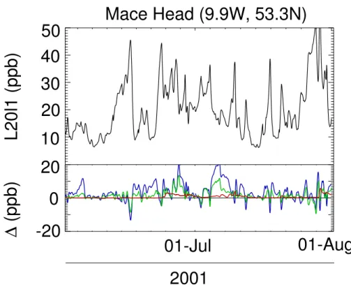
the L20L1 concentration fields which causes annihilation of the negative and positive deviations. The consequence is that, when the concentrations are sampled at Mace Head (see Fig.10), the differences between the R5 and R3 simulations are relatively small (usually smaller than 10%). Interestingly, the R5 simulation produces system-atically lower L20L1 concentrations at Mace Head. As mentioned before, more grid 20

cells fall in the high concentration end of the curve depicted in Fig.8when the North American resolved at 1◦×1◦. Consequently, less L20L1 is produced and transported towards Europe.

The differences between the R5 simulation and the simulation with only the European zoom at 3◦×2◦ active (R2, green), and the simulation with no zoom regions at all (R1, 25

blue) are also shown in Fig.10. These differences are usually much larger. This means that, at least for this artificial chemistry case, the “gain” of a better local representation is larger than the loss in accuracy that is caused by grid-coarsening at some distance from the measurement station. This observation is in line with the intuitive argument

(20)

ACPD

4, 3975–4018, 2004

that it seems not logical to resolve the atmospheric transport and chemistry globally at a high resolution when the focus is on the local situation.

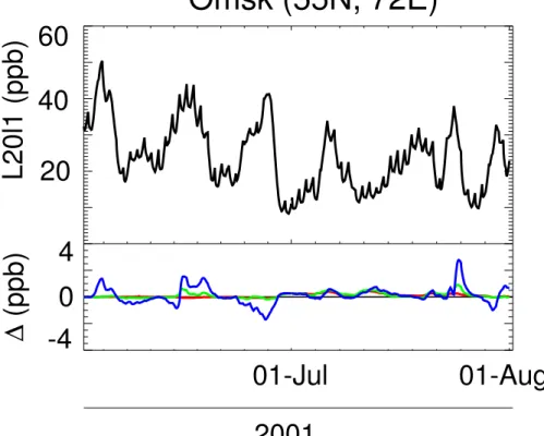
A similar conclusion can be drawn from the concentrations that are sampled at a station positioned in Omsk (see Fig.1), east of the European zoom domain (Fig.11). Since this location falls outside all zoom regions, the concentrations are only available 5

only on the 6◦×4◦model grid for all experiments (R1, R2, R3, R5). The differences be-tween R5 (top panel) and R3 (lower panel, red) are very small. Thus the concentrations as simulated at Omsk are hardly influenced by the presence of the North American zoom region. The effects of European zooming (R2 and R3) are only marginally larger, but may reach 10% if the European resolution is degraded to 6◦×4◦(R1, blue line). 10

In order to check the importance of the various processes, a TM5 simulation is ac-companied by a budget calculation. For the simulations described here, the budget of the boundary layer in the northern mid and high latitudes (between 30◦N and 90◦N) is analyzed. The values of the individual budget terms will depend on whether or not zoom regions are present. Table 3 lists the individual budget terms for the various 15

model simulations. Note that the initial conditions in the table already differ, because the simulation spans two months and the budget is shown for the second month. As outlined above, it is observed that zooming changes the production (and thus the con-centration) of chemically active tracers in a systematic way. Interestingly, relative large changes in the vertical transport are observed. With coarser resolution, the convec-20

tion parameterization appears to be more effective in venting the boundary layer. With higher resolution, however, the less effective convection is partly compensated by en-hanced advective vertical transport. This is expected, since the vertical motions that are associated with frontal systems are better resolved.

The same resolution dependencies are seen in the budgets of tracers L20 (see Ta-25

ble4) and L1 (not shown). In more realistic atmospheric chemistry simulations these effects will also be present, although they may be obscured by feed-back processes. For instance, the simulated concentration of the hydroxyl radical concentration (OH) will depend on the model resolution. As a consequence, the lifetime of methane and

(21)

ACPD

4, 3975–4018, 2004

other gases will also change with the grid size.

In general, the effects of model resolution on transport and specifically sub-grid ver-tical mixing has been poorly explored in global atmospheric chemistry studies. This example demonstrates the power of the TM5 model to quantify resolution dependent effects in a consistent and systematic way.

5

4. Conclusions

TM5 extends the functionality of TM3 by the possibility to zoom over specific regions. In this way, a local high resolution is achieved while the computational costs remain relatively low. The major advantage of a local high resolution is that the model grid cells are more representative for the locations at which measurements are taken, as 10

was shown by the222Rn study presented in Sect.3.1. Boundary conditions, which are important for longer lived species, are provided in a natural way, i.e. by a simulation on the parent grid which is run simultaneously. In the present study, regions with a highest horizontal resolution of 1◦×1◦ are employed, but the algorithm can easily be used for higher horizontal resolutions.

15

The TM5 model is ideally suited for budget studies. The import and export bud-gets of specific regions can be studied as was highlighted by the artificial tracer study presented in Sect. 3.2. With such studies in mind, we have pdefined zoom re-gions over Europe, North America, Africa and Asia (seehttp://www.phys.uu.nl/∼tm5). In this way, global “hot-spots” of atmospheric chemistry (high emission rates of ozone 20

precursors) can be resolved at higher resolution without dramatically increasing the computational costs. Other ongoing efforts with the TM5 model include the coupling with forecast meteorology in order to provide chemical forecasts (chemical weather) and the use of TM5 in inverse modelling studies. The use of two-way nesting is impor-tant for inverse modeling studies since emissions, resolved at higher resolution within 25

zoom regions, influence the simulated concentrations also outside these regions. Syn-thesis inversions that optimize emissions of trace gases by minimizing the differences

(22)

ACPD

4, 3975–4018, 2004

between simulations and measurements will therefore benefit from the two-way nest-ing approach (Bergamaschi et al.,2004). To further assist inverse modelling studies, the adjoint version of the TM5 transport routines have been coded and been used to calculate the sensitivity of specific measurements for upwind emissions (Gros et al.,

2003, Gros et al., submitted, 20041). Validation of the global transport using SF₆ mea-5

surements is currently ongoing (Peters et al., submitted, 2004)2. Finally, TM5 can be used to study the resolution dependence of processes. In Sect.3.2these effects were quantified by activating and deactivating zoom regions. Specifically the vertical mixing processes were shown to depend on resolution.

Appendix

10

Movie (http://www.copernicus.org/EGU/acp/acpd/4/3975/acpd-4-3975-mv01.mov) of daily L20L1 concentrations in the lowest model layer. The upper panel (R3) only the European zoom is active. In the middle panel (R5) the North American zoom regions are activated. The lowest panel depicts the differences (%) defined as 100(R5–R3)/R5. 15

1

Gros, V., Williams, J., Lawrence, M., Kuhlmann, R. v., Aardenne, J. v., Atlas, E., Chuck, A., Edwards, D. P., and Krol, M.: Tracing the Origin and Ages of Interlaced Atmospheric Pollu-tion Events over the Tropical Atlantic Ocean with in-situ Measurements, Satellites, Trajectories, Emission Inventories and Global Models, J. Geophys. Res., submitted, 2004.

2

Peters, W., Krol, M. C., Bruhwiler, L., Dlugokencky, E., Dutton, G., Hirsch, A., Michalak, A. M., Miller, J. B., Dentener, F. J., Bergamaschi, P., Velthoven, P. v., and Tans, P. P.: Towards regional scale inversion using a two-way nested global model: Characterization and transport using SF6, J. Geophys. Res., submitted, 2004.

(23)

ACPD

4, 3975–4018, 2004

Description of the movie

In the upper panel of the frames (R3) the North American zoom domain is not present. As a result, the L20L1 concentration fields retain the 6×4 block structure over this re-gion throughout the movie. After a few days, the patterns of L20L1 over North America in the R5 simulation show more fine structure, with higher maxima (e.g. 15 June, 28 5

June, 19 July at the East Coast, 23 July in Central USA). Interestingly, at the west coast of the USA, the R5 simulation clearly shows systematically lower L20L1 con-centrations. In that region, L1 is emitted in relatively stagnant air (Los Angeles area). The L1 concentrations in the high resolution R5 simulation reach very high levels, i.e. beyond the concentrations at which L20L1 is produced most efficiently (1000 ppt, see 10

Fig. 8). In the R3 simulation, artificial spread of the L1 emissions leads to spurious dilution and hence lower L1 concentrations over the emission hot-spots. As a result, systematically less L20L1 is produced in the R5 simulation. Clearly, the interaction be-tween meteorology and emissions plays an important role in the non-linear chemical production of L20L1 (and ozone). At the east coast, both the meteorological variability 15

and the area with substantial L1 emissions are larger.

The main transport routes out of the North American zoom region are to the north-east towards Europe and to the south-west towards the Pacific. These transport events are variable and depend strongly on the atmospheric circulation. Transport events are clearly visible in the difference plot that is depicted in the lower panel. Due to less 20

production of L20L1 in the R5 simulation, it appears as if the negative deviations are transported out of the North American domain. Differences as large as −10% are seen towards Europe (25 June, 7 July, 11 July, 30 July) and the Central Pacific (20 June, 1 July, 30 July).

Because of two-way nesting, air flowing out from a zoom domain may flow in again 25

later. This is most clearly observed in the difference movie, where the perturbations seem to “flow in” at the south-eastern side of the North American domain. From the difference movie it is also clear that the differences between the R3 and R5 simulations

(24)

ACPD

4, 3975–4018, 2004

are generally small over most of Asia and Russia. TM5 input fields

Table5 lists the TM5 input fields. These fields are produced in a pre-processing step (see Sect.2.4) that uses ECMWF data. Only a subset of all the surface fields is listed. The complete set of surface fields contains parameters that are needed for deposition 5

calculations, such as surface roughness, surface stress, sea ice, etc.

Acknowledgements. Financial support for M. Krol was provided by the European FP5 project

PHOENICS. M. Botchev, P. Berkvens and J. Verwer are acknowledged for their work on the nu-merical foundations of the zoom algorithm. Computer facilities were provided by the Dutch NCF (Nationale computerfaciliteiten). S. Wagner is acknowledged for his constructive comments on 10

the manuscript. N. Mihalopoulos (ECPL, University at Crete) is acknowledged for providing the

222

Rn measurements from Finokalia.

References

Bauer, S. E. and Langmann, B.: Analysis of a summer smog episode in the Berlin-Brandenburg region with a nested atmosphere-chemistry model, Atmos. Chem. Phys., 2, 259–270, 2002. 15

3978

Bergamaschi, P., Hein, R., Heimann, M., and Crutzen, P. J.: Inverse modeling of the global CO cycle 1. Inversion of CO mixing ratios, J. Geophys. Res., 105, 1909–1927, 2000. 3977

Bergamaschi, P., Behrend, H., and Jol, A.: Inverse modelling of national and EU greenhouse gas emission inventories, report of workshop ”inverse modelling for potential verification of 20

national and EU bottom-up GHG inventories, Tech. rep., JRC, 20, 2004. 3995

Berkvens, P. J. F., Botchev, M. A., Lioen, W. M., and Verwer, J. G.: A zooming technique for wind transport of air pollution, MAS-R9921, 31, CWI, Amsterdam, 1999. 3979,3980,3981,

3982

Berkvens, P. J. F., Botchev, M. A., Krol, M. C., Peters, W., and Verwer, J. G.: Solving vertical 25

(25)

ACPD

4, 3975–4018, 2004

and G. Carmichal, 130 of IMA Volumes in Mathematics and its Applications, 1–20, Springer, Berlin, 2002. 3982

Bousquet, P., Peylin, P., Ciais, P., Quere, C. L., Friedlingstein, P., and Tans, P. P.: Regional changes in carbon dioxide fluxes of land and oceans since 1980, Science, 290, 1342–1346, 2000. 3977

5

Bregman, A., Krol, M. C., Teyss `edre, H., Norton, W. A., Iwi, A., Chipperfield, M., Pitari, G., Sundet, J. K., and Lelieveld, J.: Chemistry-transport model comparison with ozone obser-vations in the midlatitude lowermost stratosphere, J. Geophys. Res., 106, 17 479–17 496, 2001. 3986

Bregman, B., Segers, A., Krol, M., Meijer, E., and Velthoven, P. v.: On the use of mass-10

conserving wind fields in chemistry-transport models, Atmos. Chem. Phys., 3, 447–457, 2003. 3986

Broek, M. M. P. v. d., Aalst, M. K. v., Bregman, A., Krol, M., Lelieveld, J., Toon, G. C., Garcelon, S., Hansford, G. M., Jones, R. L., and Gardiner, T. D.: The impact of model grid zooming on tracer transport in the 1999/2000 Arctic polar vortex, Atmos. Chem. Phys., 3, 1833–1847, 15

2003. 3979,3981

Cosme, E., Genthon, C., Martinerie, P., Boucher, O., and Pham, M.: The sulfer cycle at high-southern latitudes in the LMD-ZT General Circulation Model, J. Geophys. Res., 107, 4690, doi:10.1029/2002JD002 149, 2002. 3978

Cotton, W. R., Pielke, R. A., Walko, R. L., Liston, G. E., Tremback, C. J., Jiang, H., McAnelly, 20

R. L., Harrington, J. Y., Nicholls, M. E., Carrio, G. G., and McFadden, J. P.: RAMS 2001: Current status and future directions, Meteorol. Atmos. Phys., 82, 5–29, 2003. 3978

Dentener, F., Weele, M. v., Krol, M., Houweling, S., and Velthoven, P. v.: Trends and inter-annual variability of methane emissions derived from 1979–1993 global CTM simulations, Atm. Phys. Chem., 3, 73–88, 2003. 3980

25

Dentener, F. J., Feichter, J., and Jeuken, A. B. M.: Simulation of transport of222Rn using on-line and off-on-line global models at different horizontal resolutions, Tellus, 51B, 572–602, 1999.

3984,3988

Dlugokencky, E., Houweling, S., Bruhwiler, L., Masarie, K. A., Lang, P. M., Miller, J. B., and Tans, P. P.: Atmospheric methane levels off: Temporary pause or a new steady-state?, 30

Geophys. Res. Lett., 20, 1992, doi:10.1029/2003GL018 126, 2003. 3977

Frohn, L. M., Christensen, J. H., Geels, J., Brandt, C., and Hansen, K. M.: Validation of a 3-D hemispheric nested air pollution model, Atmos. Chem. Phys. Discuss., 3, 3543–3588, 2003.

(26)

ACPD

4, 3975–4018, 2004

3978

Grell, G. A., Emeis, S., Stockwell, W. R., Schoenemeyer, T., Forkel, R., Michalakes, J., Knoche, R., and Seidl, W.: Application of a multiscale, coupled MM5/chemistry model to the complex terrain of the VOTALP valley campaign, Atmos. Environ., 34, 1435–1453, 2000. 3978

Gros, V., Williams, J., Aardenne, J. A. v., Salisbury, G., Hofmann, R., Lawrence, M. G., 5

Kuhlmann, R. v., Lelieveld, J., Krol, M., Berresheim, H., Lobert, J. M., and Atlas, E.: Origin of anthropogenic hydrocarbons and halocarbons measured in the summertime European outflow (on Crete in 2001), Atmos. Chem. Phys., 3, 1223–1235, 2003. 3995

Heimann, M., Monfray, P., and Polian, G.: Long-range transport of222Rn – a test for 3D tracer models, Chem. Geology, 70, 98–98, 1988. 3979

10

Holtslag, A. A. M. and Moeng, C.-H.: Eddy diffusivity and countergradient transport in the convective atmospheric boundary layer, J. Atmos. Sci., 48, 1690–1698, 1991. 3984

Houweling, S., Dentener, F., and Lelieveld, J.: The impact of nonmethane hydrocarbon com-pounds on tropospheric photochemistry, J. Geophys. Res., 103, 10 637–10 696, 1998. 3979

Houweling, S., Kaminski, T., Dentener, F., Lelieveld, J., and Heimann, M.: Inverse modeling of 15

methane sources and sinks using the adjoint of a global transport model, J. Geophys. Res., 104, 26 137–26 160, 1999. 3977

Jacob, D. J., Crawford, J. H., Kleb, M. M., Connors, V. S., Bendura, R. J., Raper, J. L., Sachse, G. W., Gille, J. C., Emmons, L., and Heald, C. L.: Transport and chemical evolution over the Pacific (TRACE-P) aircraft mission: Design, execution, and first results, J. Geophys. Res., 20

108, 8781, doi:10.1029/2002JD003 276, 2003. 3976

Jonson, J. E., Sundet, J. K., and Tarras ´on, L.: Model calculations of present and future levels of ozone and ozone precursors with a global and a regional model, Atmos. Environ., 35, 525–537, 2001. 3978

Kaminski, T., Heimann, M., and Giering, T.: A coarse grid three-dimensional global inverse 25

model of the atmospheric transport, 2, Inversion of the transport of CO2 in the 1980s, J. Geophys. Res., 104, 18 555–18 581, 1999. 3977

Kouvarakis, G., Tsigaridis, K., Kanakidou, M., and Mihalopoulos, N.: Temporal variations of surface regional background ozone over Crete Island in the southeast Mediterranean, J. Geophys. Res., 105, 4399–4407, 2000. 3987

30

Krol, M., Peters, W., Berkvens, P., and Botchev, M.: A new algorithm for two-way nesting in global models: principles and applications, in Proceedings 2nd Int. Conf. Air Pollution Mod-elling and Simulation, April 9–12, 2001, edited by B. Sportisse, 225–235, Springer, Berlin,

(27)

ACPD

4, 3975–4018, 2004

Heidelberg and New York, 2002. 3979,3980,3983

Krol, M. C., Lelieveld, J., Sturrock, G., Penkett, S., Brenninkmeijer, C., Gros, V., Williams, J., and Scheeren, H.: Continuing emissions of methyl chloroform from Europe, Nature, 421, 131–135, 2003. 3979

Langmann, B., Bauer, S. E., and Bey, I.: The influence of the global photochemical composition 5

of the troposphere on European smog, Part I, Application of a global to mesoscale model chain, J. Geophys. Res., 108, 4146, doi:10.1029/2002JD002 072, 2003. 3978

Lelieveld, J., Berresheim, H., Borrmann, P. J. C. S., Dentener, F. J., Fischer, H., Feichter, J., Flatau, P. J., Heland, J., Korrmann, R. H. R., Lawrence, M. G., Levin, Z., Markowicz, K. M., Mihalopoulos, N., Minikin, A., Ramanathan, V., M, d., Roelofs, G. J., Scheeren, H. A., 10

Sciare, J., Schlager, H., Schultz, M., Siegmund, P., Steil, B., Stephanou, E. G., Stier, P., M, M. T., Warneke, C., Williams, J., and Ziereis, H.: Global air pollution crossroads over the Mediterranean, Science, 298, 794–799, 2002a. 3976,3979,3987

Lelieveld, J., Peters, W., Dentener, F. J., and Krol, M. C.: Stability of tropospheric hydroxyl chemistry, J. Geophys. Res., 107, 4715, doi:10.1029/2002JD002 272, 2002b. 3980

15

Logan, J. A.: An analysis of ozonesonde data for the troposphere: Recommendations for testing 3-D models and development of a gridded climatology for tropospheric ozone, J. Geophys. Res., 104, 16 115–16 150, 1999. 3977

Louis, J. F.: A parametric model of vertical eddy fluxes in the atmosphere, Boundary Layer Meteor., 17, 187–202, 1979. 3984

20

Mihalopoulos, N., Stephanou, E., Kanakidou, M., Pilitsidis, S., and Bousquet, P.: Tropospheric aerosol ionic composition in the Eastern Mediterranean region, Tellus, 49B, 314–326, 1997.

3987

Novelli, P. C., Masarie, K. A., Lang, P. M., Hall, B. D., Myers, R. C., and Elkins, J. W.: Reanalysis of tropospheric CO trends: Effects of the 1997–1998 wildfires, J. Geophys. Res., 108, 4464, 25

doi:10.1029/2002JD003 031, 2003. 3977

Olivier, J. G. and Berdowski, J.: in The Clamate System, edited by Berdowski, J., Guicherit, R., and Heij, B. J., 33–78, Balkema/Swets & Zeiringer, Lisse, 2001. 3990

Peters, W., Krol, M., Dentener, F., Thompson, A. M., and Lelieveld, J.: Chemistry-transport modeling of the satellite observed distribution of tropical tropospheric ozone, Atm. Phys. 30

Chem., 2, 103–120, 2002. 3980

Petersen, A. C., Spee, E. J., Dop, H. v., and Hundsdorfer, W.: An evaluation and intercompar-ison of four new advection schemes for use in global chemistry models, J. Geophys. Res.,

(28)

ACPD

4, 3975–4018, 2004

103, 19 253–19 269, 1998. 3983

Prather, M.: Numerical advection by conservation of second order moments, J. Geophys. Res., 91, 6671–6681, 1986. 3983

Prinn, R. G., Weiss, R. F., Fraser, P. J., Simmonds, P. G., Cunnold, D. M., Alyea, F. N., O’Doherty, S., Salameh, P., Miller, B. R., Huang, J., Wang, R. H. J., Hartley, D. E., Harth, 5

C., Steele, L. P., Sturrock, G., Midgley, P. M., and McCulloch, A.: A history of chemically and radiatively important gases in air deduced from ALE/GAGE/AGAGE, J. Geophys. Res., 105, 17 751–17 792, 2000. 3977

R ¨odenbeck, C., Houweling, S., Gloor, M., and Heimann, M.: CO₂ flux history 1982–2001 inferred from atmospheric data using a global inversion of atmospheric transport, Atmos. 10

Chem. Phys., 3, 1919–1964, 2003. 3977

Russel, G. and Lerner, J.: A new finite-differencing scheme for the tracer transport equation, J. Appl. Meteorol., 20, 1483–1498, 1981. 3983,3988

Segers, A., Velthoven, P. v., Bregman, B., and Krol, M.: On the computation of mass fluxes for Eulerian transport models from spectral meteorological fields, in Proceedings of the 2002 15

International Conference on Computational Science, Lecture Notes in Computer Science (LNCS), Springer Verlag, 2002. 3985,3986

Soulhac, L., Puel, C., Duclaux, O., and Perkins, R. J.: Simulations of atmospheric pollution in Greater Lyon, An example of the use of nested models, Atmos. Environ., 37, 5147–5156, 2003. 3978

20

Stohl, A., Eckhardt, S., Forster, C., James, P., and Spichtinger, N.: On the pathways and timescales of intercontinental air pollution transport, J. Geophys. Res., 107, 4684, doi:10.1029/2001JD001 396, 2002. 3977

Strang, G.: On the construction and comparison of difference schemes, SIAM J. Num. Anal., 5, 506–517, 1968. 3982

25

Taghavi, M., Cautenet, S., and Foret, G.: Simulation of ozone production in a complex circula-tion regime using nested grids, Atmos. Chem. Phys. Discuss., 3, 3833–3867, 2003. 3978

Tang, Y.: A case study of nesting simulation for the Southern Oxidants Study 1999 at Nashville, Atmos. Environ., 36, 1691–1705, 2002. 3978

Tiedtke, M.: A comprehensive mass flux scheme for cumulus parameterisation in large scale 30

models, Mon. Wea. Rev., 177, 1779–1800, 1989. 3984

Trickl, T., Cooper, O. R., Eisele, H., James, P., M ¨ucke, R., and Stohl, A.: Intercontinental transport and its influence on the ozone concentrations over central Europe: Three case

(29)

ACPD

4, 3975–4018, 2004

studies, J. Geophys. Res., 108, 8530, doi:10.1029/2002JD002 735, 2003. 3977

Verwer, J. G., Spee, E. J., Blom, J. G., and Hundsdorfer, W.: A second order Rosenbrock method applied to photochemical dispersion problems, SIAM J. Sci. Comp., 20, 1456–1480, 1999. 3980

Wang, Y., Shim, C., Blake, N., Blake, D., Cho, Y., Ridley, B., Dibb, J., Wimmers, A., Moody, J., 5

Flocke, F., Weinheimer, A., Talbot, R., and Atlas, E.: Intercontinental transport of pollution manifested in the variability and seasonal trend of springtime O3 at northern middle and high latitudes, J. Geophys. Res., 108, 4683, doi:10.1029/2003JD003 592, 2003. 3977

Wenig, M., Spichtinger, N., Stohl, A., Held, G., Beirle, S., Wagner, T., J ¨ahne, B., and Platt, U.: Intercontinental transport of nitrogen oxide pollution plumes, Atmos. Chem. Phys., 3, 387–393, 2003. 3977

Wild, O. and Akimoto, H.: Intercontinental transport of ozone and its precursors in a three-745

(30)

ACPD

4, 3975–4018, 2004

Table 1. Stepping order in a three-region simulation. ↓ denotes writing of boundary conditions to the children, X and Y denote horizontal advection, Z vertical advection, V vertical diffusion and convection, and C chemistry (including emissions and deposition). ↑ represents the update parent procedure. The first and last three lines represent the first and second half of the time step, respectively.

t ... t+ ∆T/2 region 1 ↓X↓YZ ... VC region 2 ...↓X↓YZ...VC CVZ↓Y↓X...↑... region 3 ...XYZVC CVZYX↑...CVZYX XYZVC↑... t+ ∆T/2 ... t + ∆T region 1 CVZ↓Y↓X... region 2 ...CVZ↓Y↓X...↓X↓YZ...VC↑ region 3 ...CVZYX XYZVC↑...XYZVC CVZYX↑...

(31)

ACPD

4, 3975–4018, 2004

Table 2. Schematic description of advection at the interface between parent (P) and child (C). Step Description

1 The parent writes boundary conditions in the appropriate cells of the child (↓) P1 is copied to C0; P2 is spread over C1, C2, and C3

2 The parent is advected∆T/2 (X) 3 ....

4 The entire parent flux at the P1-P2 boundary is applied at the C0–C1 boundary of the interface cells From the C3–C4 boundary on, advection with the child time step∆T/4

5 ....

6 From the C3–C4 boundary on, a second advection step with the child time step∆T/4 Now, the flux is set to zero at the C0–C1 boundary

7 ....

8 The child cells are used to update the tracer masses of the parent (↑) P2 becomes C1+C2+C3, P3 becomes C4+C5+C6, etc.