Coherent control of quantum information

Coherent Control of Quantum Information

MASSACHUSEITS MASSACHUSETS INSTITUTE. OF TECHNOLOGY

OCT

1 2 2007

LIBRARIES

by

Michael Kevin Henry, Jr.

Submitted to the Department of Nuclear Science and Engineering

in partial fulfillment of the requirements for the degree of

Doctor of Philosophy in Nuclear Science and Engineering

at the

MASSACHUSETTS INSTITUTE OF TECHNOLOGY

June 2007

@

Massachusetts Institute of Technology 2007. All rights reserved.

."A

A uthor ... i... i...T...

Department of Nuclear Science and Engineering

April 30, 2007

Certified by...

...

...

Davpd

.

Cory

Professor

Thesis Supervisor

R ead by ...

...

Alan Jasanoff

Assistant Professor

Accepted by ...

...

.. .

...

Jeffrey A. Coderre

Chairman, Department Committee on Graduate Students

Coherent Control of Quantum Information

by

Michael Kevin Henry, Jr.

Submitted to the Department of Nuclear Science and Engineering on April 30, 2007, in partial fulfillment of the

requirements for the degree of

Doctor of Philosophy in Nuclear Science and Engineering

Abstract

Quantum computation requires the ability to efficiently control quantum information in the presence of noise. In this thesis, NMR quantum information processors (QIPs) are used to study noise processes that compromise coherent control, to develop useful techniques for detecting noise, and to explore effective noise-protection schemes.

A quantum simulation of the quantum sawtooth map in the perturbative parameter regime is used to study the effects of experimental noise on quantum localization, a highly sensitive quantum interference phenomenon that depends on the coherence of the localized state. Experimental data and numerical simulations show that the decoherent noise known to act on the system is relatively inconsequential in this implementation of the map, and that incoherent noise is the biggest challenge to implementing localization.

While many incoherent processes appear decoherent, there are important differences. The distribution functions underlying incoherent processes are either static or slowly vary-ing and so the errors introduced by these distributions are refocusable. The influence of incoherent noise is further explored in an experimentally implemented entangling operation, where incoherence can be difficult to separate from decoherence. By studying the fidelity decay under the cyclic entangling map, the effects of incoherence are easily distinguished from decoherence in experimental data.

Decoherence free subspaces (DFSs) provide some of the most efficient schemes of avoid-ing decoherence from noise sources with underlyavoid-ing symmetries. To achieve an internal Hamiltonian structure that naturally fits a DFS encoding over a well-defined Hilbert space, we employ liquid crystal solvents to partially align a four-proton spin system, reintroducing the spin-spin dipolar couplings. In these experiments, enhanced coherent control is achieved by encoding logical qubits in a DFS. Robust control sequences enable high fidelity control in the DFS even when the system Hamiltonian is known with some uncertainty.

Thesis Supervisor: David G. Cory Title: Professor

Acknowledgments

I would like to thank David Cory for giving me the opportunity to work with him and the Cory group, and for all of the advice and instruction David has given during my years as a graduate student. David's integrity, energy, wisdom and kindness have truly inspired me.

I am thankful to many research collaborators and friends who contributed to the work described in this thesis - Sekhar Ramanathan, Joseph Emerson, Jonathan Hodges, Paola Cappellaro, Nicolas Boulant, Yaakov Weinstein, Alexey Gorshkov, Tim Havel, Colm Ryan, Mike Ditty, and Rudy Martinez.

I would also like to thank other Cory group members whom I have had the pleasure of working with - _{Deborah Chen, Jennifer Choy, Matthew Davidson, Anatoly Dementyev,} Louis Fernandes, Daniel Greenbaum, Kai Iamsumang, Benjamin Levi, Cecilia Lopez, T. S. Mahesh, Kota Murali, Dmitry Pushin, Suddha Sinha, and Sergio Valenzuela. Special thanks to Jamie Yang, Troy Borneman and Hyungjoon Cho for helping out with many

successful helium fills.

I am especially thankful to my very good friends and co-members of Graduate Lunch Seminar - Jamie Yang, Leeland Ekstrom, Alex Ince-Cushman, and Jonathan Hodges. Mem-ories of quizbowl and our weekly meetings at Sunny's will always be dear to me.

I would like to thank my friends and family at home in Texas and in Colorado for their support and encouragement. Words cannot express my gratitude for my loving wife Brook, whose endless patience, kindness, and encouragement have been my source of strength and happiness through graduate school. Finally, I am thankful to God my Creator for His grace through Christ and for a life of abundant blessing.

Dedicated to my wife Brook, the only one I see."

Contents

1 Introduction 17

1.1 Quantum information processors . . . . 18

1.2 Toward more qubits and larger systems . . . . 19

2 Localization in the quantum sawtooth map 21 2.1 The sawtooth map ... 23

2.2 Implementation details ... ... 26 2.3 Numerical simulation ... ... 32 2.4 Experimental results ... . 36 2.5 D iscussion . . . . . 37 2.6 Conclusions . . . . 42 3 Signatures of incoherence 43 3.1 Identifying incoherence by fidelity decay . . . . 44

3.1.1 Decoherent noise . . . . 45

3.1.2 Incoherent noise . . . . 47

3.2 Experim ent . . . . 49

3.3 Numerical simulation . . . . 51

3.4 Results and discussion . . . . 54

3.5 Conclusions . . . . 57

4 Liquid crystal solvent NMR QIPs 59 4.1 NMR with liquid crystal solvents . . . . 59

4.2 Dipolar coupling in a partially oriented system . . . . 62

5 Enhanced control by logical qubit encoding 71 5.1 System model ... ... 71 5.2 Experim ent . .. . ... .. .. . .. . ... . .... .. ... . . .. .... 74 5.3 A nalysis . . . . 77 5.4 Conclusions . . . . 79 6 Future direction 81 6.1 Larger Hilbert spaces ... ... 81

6.2 Limited addressability . . . . 82

6.3 Complex dynamics . . . . 83

6.4 Conclusions . . . . 83

A Fidelity of logical qubit control 87 A.1 M easures of control . . . . 87

List of Figures

2-1 The momentum distribution after 0, 5, 10, and 40 iterations of the classical and quantum sawtooth maps. The classical map is chaotic, which causes the distribution to diffusively broaden. The quantum map causes localization, and the breadth of the distribution is essentially static.. . . . . 25

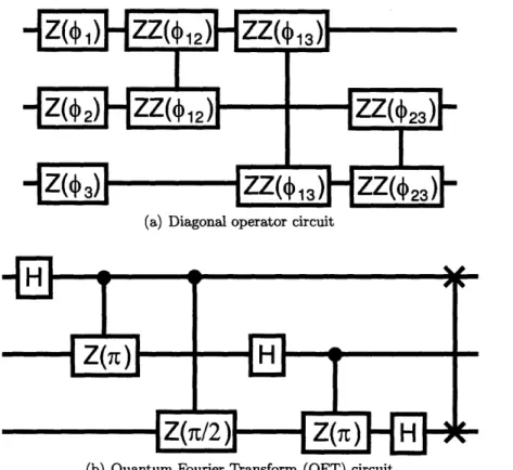
2-2 Quantum circuits for implementing the quantum sawtooth map: the quan-tum Fourier transform and a generalized diagonal unitary operator. These circuits enable a computationally efficient quantum simulation of the quan-tum sawtooth map. . . . . 27

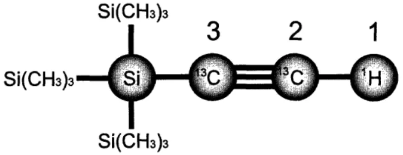
2-3 A diagram of the tris(trimethylsilyl)silane-acetylene molecule used to simu-late the quantum sawtooth map in a liquid state NMR QIP. . . . . 30

2-4 The hydrogen and carbon rf control fields versus time for the full quantum sawtooth map pulse sequence. . . . . 31 2-5 The nine point distribution of carbon rf powers measured in previous

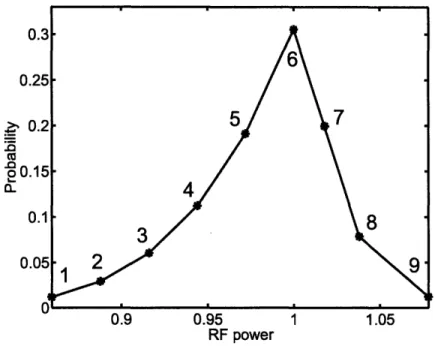
experi-ments and used to simulate the experimentally implemented control sequence for the quantum sawtooth map . . . .. . . . . 34

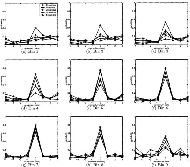
2-6 Momentum distributions for different regions of the ensemble generated by numerical simulations of the experiment which account for T1 and T2 deco-herence. Each plot represents the momentum distribution resulting from a numerical simulation of the control sequence with a different carbon rf power. In experiments, the weighted average over the incoherence is observed. . . . 35 2-7 The momentum distribution observed in the experiment and in various

nu-merical simulations of the experiment after zero through three iterations of the quantum sawtooth map. . . . . 36

2-8 The full width at half maximum (FWHM) of the momentum distribution after zero through four iterations of the sawtooth map in various implemen-tations. The FWHM reveals that despite the noise affecting the QIP, the distribution mimics the ideal quantum behavior, and does not diffusively broaden as in the classical case. . . . . 38 2-9 The second moment of the momentum distribution determined from

numeri-cal simulations of the quantum sawtooth map experiment including the error models discussed in the text, compared to the ideal data and the experimental data. This plot demonstrates the relative importance of the individual noise mechanisms as they contribute to the experimentally observed delocalization process. . . . . 39 2-10 The magnitude of each element of the superoperators and most significant

Kraus operators for numerical simulations of the quantum sawtooth map experiment, including different types of errors. . . . . 41

3-1 The quantum circuit for exploring incoherence in an entangling operation on a QIP. The circuit creates a maximally entangled GHZ state, to which

4n iterations of a two-qubit entangling operation are applied. The resulting

entangled state is then converted to a computational basis state. . . . . 50 3-2 A diagram of the tris(trimethylsilyl)silane-acetylene molecule used to

imple-ment the quantum circuit in Fig. 3-1 in a liquid state NMR QIP. . . . . 51 3-3 The distribution of carbon rf powers measured in previous experiments and

used in numerical simulations of the NMR implementation of the circuit in Fig. 3-1.. ... ... ... 52 3-4 The fidelity decay from a numerical simulation of the experiment, where rf

inhomogeneity is simulated using two different models. Comparison of the two plots shows that the fidelity decay recurrences are caused by incoherent noise. . . . . 53 3-5 The sum of the absolute value of the density matrix components measured

in the experiment and in numerical simulations. This plot shows that inco-herence in the entangling operation appears with distinct signatures in the experim ental data. . . . . 55

3-6 The Fourier transform of each experimentally measured component of the density matrix, compared to numerical simulations of the experiment using two models of rf inhomogeneity discussed in the text. This plot shows that incoherence in the experimentally implemented entangling operation appears as high frequency components in the Fourier transform of a state fidelity m easurem ent. . . . . 56

4-1 Illustration of the order properties of a nematic liquid crystal phase, showing orientational but not positional ordering. Solutes dissolved in a nematic liq-uid crystal adopt preferred orientations that restrict thermal rotation, caus-ing nuclear spins within the molecule to retain non-zero dipolar interactions which are not present in an isotropic liquid. . . . . 60

4-2 600 MHz proton spectrum of o-chloronitrobenzene (CNB) partially oriented by the liquid crystal solvent ZLI-1132 showing suppression of the baseline signal caused by the solvent material. The baseline is suppressed by the Cory-48 pulse sequence, parameterized to refocus the dipolar couplings among solute protons but not among solvent protons . . . . 61

4-3 Coordinate frames used in the expression of the order parameter, which de-termines the intramolecular nuclear spin dipolar coupling strengths. .... 63

4-4 600 MHz proton spectrum of benzene partially oriented by the liquid crystal solvent ZLI-1132. . . . . 65

4-5 Comparison of three regimes of NMR QIP, showing liquid crystal solvent NMR QIPs (LNQs) as a bridge between liquid and solid state implementa-tions. LNQs provide a natural setting for addressing some of the important challenges in solid state NMR quantum information processing. . . . . 67

5-1 _{600 MHz proton spectrum of o-chloronitrobenzene (CNB) partially oriented} by the liquid crystal solvent ZLI-1132. The inset was collected under the MREV-8 sequence, and shows the four protons uncoupled with chemical

5-2 The procedure and experimental results of creating a Bell state over two log-ical qubits encoded in the four dipolar-coupled protons of the CNB molecule. The experimentally prepared logical input state has a correlation of 0.90 with the numerically simulated logical input state. The correlation for the Bell states is 0.84. . . . . 76 5-3 Correlation of the numerically simulated and experimentally measured

den-sity matrices for the logical input state and the logical Bell state. The corre-lations are averaged over a dispersion of simulated Hamiltonian parameters. As more couplings are varied, the correlations decrease only slightly since the pulse sequences were engineered to be robust to these variations, and the loss in correlation is most pronounced for the input state. . . . . 78 5-4 Fidelity of two-qubit entangling operation pulses numerically simulated under

various conditions, comparing control of two logical qubits versus all pairs of spin qubits. The fidelity under each set of conditions is significantly better in the case of logical qubits than for any pair of spin qubits. . . . . 79

6-1 Diagram of the 4-hydroxyphenanthrene molecule which could be used as a 16 qubit heteronuclear LNQ. . . . . 82 6-2 NMR spectra for different regimes of Hamiltonians, showing addressable spins

in the liquid state, resolved spin transitions in partially oriented systems, and many equivalent spins broadened by dipolar interactions in a solid. . . . . . 84

List of Tables

Chapter 1

Introduction

Quantum systems have unique properties that are not observed in the classical, macroscopic world. Information stored in a quantum system - "quantum information" - has inherent manifestations of these unique properties and therefore has capabilities that are unparal-leled in traditional computing devices. A quantum computer harnesses the computational power of quantum systems, exploiting coherent superposition states, entanglement, and other quantum resources, to achieve an advantage over classical computers in solving certain problems, such as factoring large numbers and searching unsorted lists [42,95). The feasi-bility of quantum computation relies on the possifeasi-bility of quantum error encodings [96,100], which enable arbitrarily precise quantum computation in the presence of noise [59].

In perhaps its most important function, a quantum computer can be programmed to simulate the dynamics of other quantum systems [36, 71]. Efficient quantum algorithms have been found for simulating a variety of complex quantum systems [1, 2,40, 69,93]. In this capacity, quantum computers could provide meaningful insight into the dynamics of large quantum systems which cannot be efficiently simulated on classical computers. In the second chapter of this thesis, an experimental implementation of one such algorithm [7] which efficiently simulates the dynamics of the quantum sawtooth map is presented.

The criteria [30] necessary for utilizing the full power of quantum computation have not currently been realized in any device. However, quantum information processors (QIPs) provide an experimentally accessible means for exploring coherent quantum control and for implementing quantum algorithms. This thesis describes a number of experiments per-formed with nuclear magnetic resonance (NMR) QIPs. The ideas explored in these

ex-periments have application in ongoing efforts to engineer precise coherent control in larger systems, toward a scalable quantum computer. The QIPs used here operate with a small number of quantum bits (qubits) in highly mixed states, and they are subject to significant noise.

1.1

Quantum information processors

Experimental implementations of quantum information processing have developed in a num-ber of technologies including liquid state NMR, which allows precise coherent control of small networks of weakly coupled nuclear spins. Liquid state NMR experiments mimic pure state quantum dynamics by utilizing isomorphic pseudopure states [20,41]. This approach has been used to successfully implement a variety of quantum information concepts including quantum error correction [11, 23], the Deutsch-Jozsa algorithm [50], the quantum Fourier transform [117), Shor's factoring algorithm [108], quantum process tomography [115], noise-less subsystems [38,110], decoherence free subspaces [37,49], various simulations of quantum dynamics [17,98,107,116], and studies of quantum entanglement [9,105] including experi-ments with up to twelve qubits [81].

A number of approaches have been developed for reducing the effects of noise in QIPs, advancing the state of the art in these devices. Strongly modulating pulses (SMPs) are numerically optimized rf control fields which implement precise, spin-selective control, av-eraging out all unwanted time evolution in the system while minimizing the effects of deco-herence [37). Gradient ascent pulse engineering (GRAPE) has also been used to design nu-merically optimized pulse sequences which implement precise unitary operators [54]. In ad-dition, quantum error-correcting codes [96,100], noiseless subsystems [58,122], decoherence free subspaces [32,70,122], dynamical decoupling [109,111-113], composite pulses [24,68], and robust pulses [88], have all been developed for protecting quantum information against noise and decoherence. The noise protection scheme most appropriate for a given system is generally determined by the noise model, since each scheme is best suited for certain types of noise. In Chapter Three of this thesis, a discussion of incoherent noise is presented, along with a method for identifying its presence in a QIP, so that the appropriate noise protection scheme may be chosen.

1.2

Toward more qubits and larger systems

While liquid state NMR systems provide a useful testbed for quantum computation and continue to yield meaningful progress, they are fundamentally limited in their scalabil-ity - their potential to efficiently incorporate more qubits. As the number of qubits in a liquid state NMR QIP increases, the signal decreases exponentially [114]. Many of the pro-posed scalable approaches to nuclear spin-based quantum computing envision solid state implementations [21,52,55, 62,94, 101]. Solids are composed of large networks of dipolar-coupled nuclear spins, and a principal challenge in these systems is controlling the multispin dynamics. While methods for coherent control of solid state nuclear spin systems have pro-gressed [4,5,89], incorporating all the desired capabilities of a quantum computer remains a challenge.

Liquid crystal solvent NMR QIPs [72, 120] provide an intermediate ground between liquid and solid state implementations. Molecules dissolved in liquid crystalline material contain networks of dipolar-coupled spins that, to a good approximation, are uncoupled from their environment [34]. The network of spins is effectively limited to single molecules, and each spin in a molecule may have a unique resonance frequency, thus the multispin dynamics are more easily controlled than in solids. While liquid crystal solvent NMR QIPs are not scalable, they do present the possibility of modestly increasing the size of exper-imentally accessible Hilbert spaces, since interactions are mediated by strong long-range dipolar couplings and are not limited to bond-mediated scalar couplings as in liquids. Liq-uid crystals offer a more tractable setting for studying dipolar-coupled spin networks, while maintaining sufficient complexity to provide meaningful contributions to scalable systems.

The second section of this thesis has three parts: Chapter Four introduces fundamentals of liquid crystal solvent NMR QIPs, Chapter Five describes an implementation of two logical qubits using this technology, and Chapter Six suggests a future direction of these studies and how they might contribute to progress in the broader efforts of the quantum computing community.

Chapter 2

Localization in the quantum

sawtooth map

The development of quantum computers promises a new approach for exploring quantum mechanics in complex systems. In the future, we hope to use quantum computation to emulate quantum behavior in Hilbert spaces that are larger than can be simulated on a classical computer. Today we have access to QIPs that are prototypes of quantum comput-ers (QCs). These devices operate over small and limited Hilbert spaces, and with significant noise. However, even with these limitations they can be used to explore questions of quan-tum mechanics that start to reflect the power we expect of future QCs. Even when QIPs operate on highly mixed states, as is the case for liquid state NMR implementations, we can distill properties that are consistent with the desired quantum phenomena. Here we will explore one such example, localization under the quantum sawtooth map. Localization is a uniquely quantum phenomenon and thus a natural target of quantum computation.

- Dynamical localization occurs in classically chaotic quantum maps, in which the quan-tum state initially diffuses at the classical rate due to repeated quasi-random perturbations, but then stabilizes to a fixed probability distribution and remains coherently localized un-der subsequent perturbations [16]. In the case of perturbative localization, the probability distribution is localized with no initial period of diffusion. In both cases, the exponen-tially peaked, static probability distribution distinctly contrasts with the classical, diffusive behavior. Efficient algorithms have been developed for simulating the dynamics of local-ization in the kicked rotator model [39], the quantum sawtooth map [7], and the kicked

Harper model [66] on a QIP. Although localization can in principle be observed in an ideal emulation using as few as three qubits [6], the sensitivity of this phenomenon to noise ef-fects [6,7,65-67,84,99] poses a rigorous challenge in the task of creating and maintaining a localized state on a noisy QIP.

In our experiment, we explored localization on a small (3-qubit) QIP based on liquid state NMR [48]. The aim of the study was to implement the sawtooth map on our QIP, to do so in such a way that we observe properties of localization which are clearly distinct from the classical behavior, and to use this example emulation as a test of the precision of our implementation as well as to motivate the continued refinement of this implementation.

Since liquid state NMR QIP relies on a large spatially distributed ensemble of quantum systems, we have to be careful in selecting the measures that we use for observing localiza-tion. The errors in our implementation of the sawtooth map will vary over the ensemble due to the inhomogeneity of the rf control field. There will be regions of the ensemble where the fidelity of implementation of the sawtooth map is sufficient that we observe lo-calization, while for other regions the errors will be large enough to prevent localization. In the experiment we observe the sum of these effects, and thus we expect to see a peak in the probability distribution in the basis of localization that is representative of those parts of the ensemble that are localized, accompanied by a background offset in the probability distribution in the basis of localization resulting from those parts of the ensemble that are not localized.

A description of the sawtooth map is given in Sec. 2.1, followed by an explanation of the experimental implementation of the map in Sec. 2.2. A discussion of the noise effects expected in the experiment are presented in Sec. 2.3, along with a discussion of their effects on the localization phenomenon. In Sec. 2.4 the experimental results are reported and shown to demonstrate properties which are consistent with localization. The results are further compared with numerical simulations of the experiment which show that the imperfections in the data are well accounted for by the error model identified in previous work [10,88, 115]. Finally, in Sec. 2.5, numerical studies of the error model are applied to

2.1

The sawtooth map

The sawtooth map is a periodically kicked system with period T and kick strength k, whose classical dynamics are dictated by a single parameter K = kT. One iteration of the classical

sawtooth map is compactly described by the equations

J= J+ k(E - 7r)

(2.1)

0 = E+ TJ

where

E

is the angular position variable and J is the angular momentum variable. The cylindrical phase space, which results from the periodicity of the position variable (0 ; E < 27r), can be represented on a torus by truncating the momentum space to length 27rL/T and applying a periodic boundary condition. In the quantum regime, one iteration of the sawtooth map is represented by the unitary time evolution operator

Uaw(0, T) = exp (-iTi2/2) exp (ik($ -- 7r)2/2) (2.2)

where J and

e

are conjugate action quantum mechanical operators. The state of the quantum system is represented by a density matrix ; expressed in the momentum basis. A detailed description and insightful discussion of the sawtooth map can be found in reference [6].

In a simulation of the quantum sawtooth map on an nq qubit quantum information processor, the momentum basis states of the emulated system are represented by N = 2q

computational basis states, therefore N = 27rL/T. The momentum basis states are labeled

by their eigenvalues -N/2 <

j

< N/2, such that i

j)

=

j

j).

The position basis states |06,) have eigenvalues 0m = (27rm/N), such that

e

10m)

O 0mr), where 0 < m < N. The

overlap between conjugate basis states is given by

1F27im(N

(Omj) = 1exp j + - (2.3)

VN/-

N (i

2

Quantum localization. In the classical phase space, when K < -4 or K > 0, the sawtooth map induces chaotic motion, which is seen by considering a classical ensemble of trajectories, where each element of the ensemble has a fixed initial momentum (J = 0) and

a randomized initial position (e). The chaotic motion arises due to the presence of the term

k (E - 7r) in Eq. 2.1, which gives a kick to the momentum at each iteration of the map. In chaotic parameter regimes, the strength of the sequence of kicks can be approximated as a quasi-random sequence, leading to diffusive broadening along the momentum dimension of the classical phase space, as shown in Fig. 2-1. As a result, the breadth of the distribution, as measured by its second moment, grows linearly with the number of map iterations, n, according to

((AJ)

2

₎

_P

_Dn,

(2.4)

where D ~ (ir2/3)k 2 is the classical diffusion coefficient. As the map is iterated, momentum diffusion continues indefinitely, and the probability distribution approaches uniformity over the bounded toroidal phase space.

The quantum system demonstrates a strikingly different behavior. Like the classical map, the quantum sawtooth map initially causes diffusive broadening in the momentum basis according to the classical diffusion coefficient D. However, after n* ; D iterations of the quantum map, diffusion is suppressed due to quantum interference, and for all sub-sequent iterations, the quantum state maintains roughly the same exponentially localized profile over the momentum basis. This surprising interference effect requires the coherence of the quantum state. The square root of the quantum standard deviation ( ( )2) rep-resents the number of states that are significantly populated in the system, and is essentially static after n* iterations, representing the onset of localization. Therefore, the localization length

1=

(N2)

=

Dn*

(2.5)

serves as a useful parameter for characterizing a localized state. The inverse participation ratio (IPR) is another useful quantity for describing localized states [7]. However, the IPR of a localized state is approximately half of the localization length, and the IPR has a minimum value of 1. Therefore the IPR is not useful in the parameter regime discussed here, where

1

< 2.

The heuristic approximation n* ~ D

1

1 [8] yields a theoretical prediction of the localization length based on the kick strength

1

~ (7r2/3)k 2. Quantum localization occurs when the localization length is less than the total breadth of the phase space N. However, the degree to which a physical system becomes localized may be reduced by noise effects,

as this unique quantum phenomenon is quite sensitive to decoherence and other types of errors [65,67,84,99]. This sensitivity poses a rigorous challenge when trying to create and maintain a localized state on a noisy QIP.

The implementation of the quantum sawtooth map reported here takes L = 7, K = 1.5,

N = 8, which corresponds to the classically chaotic regime, with a diffusion coefficient of

D

: (7r2/3)k2 = 0.24. The theoretical approximation that n* ~ D predicts that the system will be localized after one iteration of the map (n* < 1). This effect is known as perturbative localization, where the system is localized without the initial diffusive behavior. The results of numerical simulations plotted in Fig. 2-1 confirm this prediction, as the breadth of the probability distribution is essentially static after a single iteration of the quantum map.

Quantum

+0-

iter

0

-o-~ iter

5

-v- iter

10

-v6-

iter 40

Classical

*

iterO

+

iter

5

A

iter

10

v

iter

40

-1

0

Momentum

Figure 2-1: The momentum distribution after 0, 5, 10, and 40 iterations of the classical (red, filled markers) and quantum (blue, unfilled markers) sawtooth maps (L = 7, K = 1.5,

N = 8). The classical distribution represents 20,000 realizations of the map, with initial momenta

j

= 0 and random initial positions uniformly distributed over the phase space. The initial quantum state is the

j

= 0 momentum eigenstate. In the quantum case, the momentum is discrete, and each data point represents the population of the indicated momentum state. In the classical case, the momentum is continuous, and each data point represents the probability of momentum being in the range of the indicated value i1/2. The classical map is chaotic, which leads to the observed diffusive broadening. In the quantum map, since the localization length is less than 1, the state remains exponentially localized after a single iteration. The breadth of the momentum distribution is essentially static in the quantum case, and only the

j

= 0 momentum state is significantly populated.

2.2

Implementation details

An algorithm for the quantum sawtooth map can be generated by expressing the matrix elements of the map in the momentum basis:

(I

Usaw

|j')

=

E (j Iexp

(-iT2/2)

1m)

(9ml exp

(ik(O -

r)2/2)

lj')

= exp

(-iTj

2_/2)

_(j|6

m

)

exp

(ik(Om

- 7r)2/2)

(9mj')

=

(

UJU&TUeUQFT

Ij)

(2.6)

where UQFT is the familiar Quantum Fourier Transform (QFT) which has the action of toggling between the position and momentum basis representations, and the diagonal free evolution and kick operators, Uj and Ue, are defined

(j

Uj

lj')

=

exp (-iTj

2

/2) (jjj')

(2.7)

(9m| Ue

|0m

= exp (ik(Om - Ir)2/2) (6m|6'

).

(2.8) This form of the quantum sawtooth map (Usaw = UJU&kTUeUQFT) reveals the

un-derlying structure of the map: After the system is initialized to a momentum basis state, the first operation in the quantum sawtooth map, the QFT, transforms the system to the position basis representation, where the diagonal kick operator Ue applies an impulse force. The inverse of the QFT is applied next, returning the system to the momentum basis representation, where the diagonal free evolution operator Uj is applied. These four steps (UQFT, Ue, UkT , UJ) constitute a single iteration of the quantum sawtooth map. After iterating the map, the localized probability distribution corresponds to the diagonal elements of the density matrix, W = (jj 1j). Realizing that the only effect of the free evolution operator is to apply a phase to the coefficient of each momentum basis state, Uj can be neglected in the final iteration of the map, since a phase does not alter the measured probabilities in that basis.

Quantum circuits. A quantum circuit for the QFT is derived in [82] and shown in Fig. 2-2(b). Prior implementations and experimental analysis of the QFT are described in [115,117]. Circuits for Uj and Ue are conveniently found in realizing that any diagonal

(a) Diagonal operator circuit

(b) Quantum Fourier Transform (QFT) circuit

Figure 2-2: Quantum circuits for implementing the quantum sawtooth map. For both circuits, Z(x) on qubit

1

indicates the Z-rotation, exp(-ixUo/2). ZZ(x) on qubits 1 and k indicates the two-qubit operation exp(-ial Cz-). H indicates the Hadamard operator (a.,+

1Z')/v/2), and the two-qubit operation at the end of the QFT is the swap gate. (Top) The circuit for implementing any diagonal unitary operator. This circuit can be parameterized for either the diagonal free evolution operator Uj or the diagonal kick operator Ue using

#

21-1(a + 7#) and

#lk

= 21+k-3,, where the aj, ae, 3

j

and 3e derived in the text.

operator can be decomposed into a series of single-qubit Z-rotations and two-qubit ZZ-interactions. The quantum sawtooth map is emulated by programming the gates in Fig. 2-2(a) to implement Uj and Ue. Parameterization of the circuit follows from a decomposition

of the basis number operator M in) = m im), where 0 < m < N, into a sum of products of

spin operators

n.

MIm) =

1 - CO)2l-2m),

l=1

(2.9)

where

o1

indicates the Pauli operator

o-z

acting on the -2 @9

10

..

---

& 1, and

M|110 -.-.

0) = 2"e 110

-.-. 0).

lth qubit. For example o4ln) =

In general,

nq

exp

(-ia?[)

= exp -ia (I - a') 21-1

nq

oc exp

+ia

l1<j (2.10) (2.11) (2.12)

where oc indicates terms proportional to identity have been dropped since they have no observable effect on the quantum state. By identifying

e

=

27rM/N,

we can write the diagonal kick operator

(2.13)

(2.14)

Ue

=

exp (ik($

-

7r)2/2)

=

exp i

(

27rM

-

r

2 oc exp +i2kr2 (k2 - NM)

oc exp

+i

ao +

(

2)

30

o)01-1

-..

j=1

(=1

nq exp -ip30 2L + 30 1<j (2.15)

where we have defined

ao =

2kyr2/N (2.16)

#0

-

-2k7r 2_/N2_{. (2.17)}

Equation 2.15 indicates that Ue is implemented by n. single-qubit Z-rotations and 3n2 two-qubit ZZ-interactions. Each operation is parameterized by the values in the exponents of equation 2.15.

The parameters for implementing the diagonal free evolution operator can be found in a similar manner by recognizing that J = M - N/2, and therefore

Uj

=

exp (-iT

2/2) =

exp

iT

(M

-

Ni))

(2.18)

iT 2

oc

exp

(-

2

- N(f)

(2.19)

oc

exp

+i aj +

2

j-

#

_Z22

al

2~-2 ... (j=1

(

fq ex -i~ 2+-30,1 O _(2.20) 1<j

where we have defined

a =-

-TN/2 -rL (2.21)

,3 =- T. (2.22)

This circuit for the quantum sawtooth map is computationally efficient, in that the number of fundamental quantum gates required to implement the algorithm depends polynomially on the number of qubits [7].

NMR

QIPs.

In NMR quantum information processing, nuclear spins polarized by a strong external magnetic field serve as qubits. The molecule used in this experiment, dia-grammed in Fig. 2-3, is tris(trimethylsilyl)silane-acetylene dissolved in deuterated chloro-form. The carbon nuclei in the acetylene branch are carbon-13 enriched, and the methyl carbons are of natural isotopic abundance. The two carbon-13 nuclei and the hydrogen nucleus in the acetylene branch are used as qubits. The full internal Hamiltonian has the

Si(CH3)3

Si(CH3)3

S

CH

Si(CH3)3

Figure 2-3: A diagram of the tris(trimethylsilyl)silane-acetylene molecule used to simulate the quantum sawtooth map in a liquid state NMR QIP. The hydrogen nucleus in the acetylene branch is labeled qubit 1 in the experiment; the two carbon-13 nuclei in the acetylene branch are labeled qubits 2 and 3.

form

flq

int= Z rVor +

Z

r J Ok

(2.23)

i=1 j<k

where vi is the resonance frequency of the ith spin, and Jjk is the frequency of scalar

coupling between spins

j

and k. Note that Jjk is not related to the quantum operator

J. The hydrogen nucleus is labeled qubit number 1, making it the most significant bit

in the computational state vector. The carbon qubits are labeled as indicated in Fig. 2-3. Experiments are performed in a 9.4 Tesla magnetic field, where the Carbon qubits are separated by 1.201 kHz. The scalar couplings are J12 = 235.7 Hz, J23 = 132.6 Hz, and

J13 = 42.9 Hz. Because the spin system is in a highly mixed state at room temperature, the system was prepared in a pseudopure state [20] by the technique described in [104]. Three readout sequences were needed to measure the eight diagonal elements of the density matrix, which correspond to the distribution of momentum basis states.

Pulse sequences. The average gate fidelity [37] of each unitary control sequence was optimized over the full Hilbert space. The input state preparation pulse sequence, which is non-unitary, was optimized based on the state correlation [37] between the simulated input state

pism

and the ideal input state

pideal

= 1100) (1001. The average fidelity (or state correlation) of each implemented pulse sequence, as calculated by numerical simulation, is listed in Table 2.1. The NMR pulse sequence for one full iteration of the quantum sawtooth map is shown in Fig. 2-4.

Table 2.1: Pulse sequences designed for the quantum sawtooth map experiment. Fidelities are calculated by numerical simulations which account for rf inhomogeneity, neglecting decoherence effects.

Map

Input State Preparation QFT QFT Inverse J Diagonal

E

Diagonal

Readout 1 Readout 2 Readout 3

1

H

c

-1

1

-1

Duration (ms) 50 6

6

50 20 0.01 62 72 Fidelity Corr = 0.99 0.99 0.99 0.99 0.99 1.00 0.98 0.98

0.02

0.04

0.06

0.08

time (seconds)

Figure 2-4: The hydrogen (H) and carbon (C) rf control fields versus time for the full quantum sawtooth map pulse sequence. Red versus blue pulses are

pulses above versus below the horizontal axis are 180 degrees out frequency of each hydrogen (carbon) pulse is 46.7 kHz (17.5 kHz).

90 degrees out of phase; of phase. The nutation

2.3

Numerical simulation

Through numerical simulation of the experiment, it is possible to predict the behavior of the system under the optimized control sequence in the presence of various types of noise known to influence the QIP. Errors affecting the implementation of the quantum sawtooth map are conveniently classified in three categories [10,88, 115] -coherent errors, decoherent errors, and incoherent errors -which can be generally used to categorize the errors affecting any QIP. Each type of error delocalizes the system in a different manner.

In the presence of coherent errors, the system evolves under a unitary process other than the ideal quantum sawtooth map. Due to their unitary nature, coherent errors are reversible. The coherent errors modeled in numerical simulations arise in the experiment due to strong coupling between the carbon qubits, as well as the action of the internal Hamiltonian during rf pulses. Coherent errors delocalize the system by introducing unitary transitions between momentum states.

Decoherent errors cause the individual members of the ensemble (and hence the ob-served ensemble average) to evolve in a non-unitary fashion. Decoherent evolution can be modeled as a coupling between the system and an external environment and can usually be represented by a completely positive linear map, expressed as an N2 x N2 superoperator S acting on a columnized

N

2 _{x 1 state vector}

Ip),

_{according to}

IPout)

= $IPin) .

(2.24)

Decoherent errors are accounted for in numerical simulations by allowing the system to evolve under an approximate relaxation superoperator [35], which is completely diagonal in the generalized Pauli basis. In this diagonal form, each non-zero entry in the relaxation superoperator represents the decoherence rate of a generalized Pauli basis operator; the specific values used in simulations are based on measurements of all Tis in the three qubit system as well as the single species T2s.

Given the time scale of one full iteration of the quantum sawtooth map (10-1s) com-pared to the system's typical decoherence rates (1 s 1), decoherence in this system is in the moderately dissipative regime, which has been shown to cause delocalization in the quantum sawtooth map [65]. The non-unitary, dissipative action of decoherence along with the mixing action of the control sequence causes an essentially uniform damping of the

measured probability distribution, accompanied by a uniform background offset that con-serves probability. The background offset in probability appears in the density matrix as an increased identity component, which represents a loss of system purity and a corresponding increase in the von Neumann entropy of the system. In this way, the effect of decoherence is to mimic the diffusive, chaotic dynamics of the classical system described in Sec. 2.1.

Incoherent errors occur when the various members of the experimental ensemble ex-perience a distribution of unitary time evolution operators. Incoherent evolution can be generally expressed as an operator sum

Pouj

=

Zp(k)

UkpinU', (2.25)

k

where p(k) is the probability that a member of the ensemble will undergo unitary time evo-lution under Uk. Under incoherent errors, the individual members of the ensemble evolve coherently, but the ensemble-averaged time evolution of the system is non-unitary. The dominant incoherent errors in the experiment arise due to the inhomogeneity of the rf field over the spatial extent of the liquid state NMR sample. When an rf pulse is applied during the experiment, the members of the ensemble experience a distribution of rf powers, and only a fraction of the ensemble actually experiences precisely the nominal (ideal) rf power. In numerical simulations, we can approximate the effects of the continuous distribution of carbon rf powers by simulating a previously measured distribution of nine discrete bins of rf power, plotted in Fig. 2-5. Bin 6 represents the largest portion of the ensemble and cor-responds to the nominal rf power, while the other eight bins result from the inhomogeneity of the rf control field. In the experiment, there are two dimensions of incoherence: one for both the proton and carbon rf-control fields. In numerical simulations presented in Sections 2.4 and 2.5, the continuous distribution of carbon and hydrogen rf power correlations is approximated by a discrete two-dimensional (9 x 9) rf probability distribution function.

Simulating only the one-dimensional distribution of carbon rf power in Fig. 2-5 is sufficient for gaining a qualitative understanding of the effects of incoherent noise in the experiment. Figure 2-6 shows the results of numerical simulations of the experimentally implemented control sequence for each bin of rf power; the simulations include decoherence effects. Due to the incoherence, the local errors are different for each bin. Consequently, in regions of the ensemble where the rf power is near the nominal rf power (see Bins 6

0.9 0.95 1 1.05

RF power

Figure 2-5: The nine point distribution of carbon rf powers measured in previous ex-periments and used to simulate the experimentally implemented control sequence for the quantum sawtooth map. The carbon rf power is in units of the nominal carbon nutation frequency, 17.5 kHz. The numerals labeling each point in the distribution indicate the associated bin of incoherence in Fig 2-6.

through 8), the fidelity of implementation of the sawtooth map is sufficient that we observe localization. For other regions which constitute a smaller percentage of the ensemble (e.g. Bin 1), the errors are large enough to prevent localization and the momentum distribution is broad. Hence we see that in the experiment, when we observe the weighted average of these distributions, the (more abundant) localized portions of the ensemble will appear as a peak in the

j

= 0 momentum state, and the delocalized portions of the ensemble will contribute an approximately uniform background offset across the momentum distribution.

Another important insight gained from analyzing distributions plotted in Fig. 2-6 is that the bins where the rf power is near ideal are relatively unaffected by decoherence. Consequently, we expect incoherence rather than decoherence to be the principle source of noise compromising our ability to observe localization over the ensemble. This is discussed in more depth in Sec. 2.5.

.8 momentum state j (d) Bin 4 .8 .6, .4-.2 4 - -2 -1 0 momentum state j (g) Bin 7 208 M06 K0.4 -4 -' -2 -1 0 1 2 3 momentum state j (e) Bin 5 O.E 20. 00.4 1 2 3 24 -3 -2 -1 0 4q -3 -_2 _momentum -1 _state 0 _j (h) Bin 8 1 2 3 8 6 4 2 -4 - - -1 0 1 2 momentum state j (f) Bin 6 4 -0

2

-3 -2 -1 0 1 momentum state j (i) Bin 9

Figure 2-6: Momentum profiles for different regions of the ensemble generated by numer-ical simulations of the experiment which account for T1 and T2 decoherence. Each plot represents the momentum profile resulting from a numerical simulation of the control se-quence (zero through four iterations) with the carbon rf power indicated in Fig. 2-5. Bin 6 represents the nominal rf power, which has the highest fidelity when compared to the ideal quantum sawtooth map. The distributions simulated near the nominal rf power ap-pear to be localized, while those far from the nominal rf power are quickly delocalized. In experiments, the average over the incoherence is observed (weighted by the probability distribution in Fig. 2-5).

2 1 0 Momentum State j

(b) 1 iteration

error bar I error bar I

1 0 1 2 3 4 3 2 1 0

Momentum State j Momentum State j

(c) 2 iterations (d) 3 iterations

1 2 3

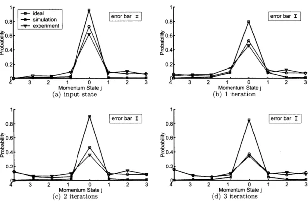
Figure 2-7: The momentum distribution after 0 through 3 iterations of the quantum saw-tooth map (L = 7, K = 1.5, N = 8) for the experiment (triangles), a numerical simulation of the experiment which is not affected by noise (squares), and finally a numerical simulation of the experiment which includes coherent errors, decoherence effects, and incoherent errors due to rf inhomogeneity in both the carbon and hydrogen control fields (circles). Error bars are drawn to scale for each iteration. The population of the initial state (j = 0) dom-inates the distribution through 3 iterations of the experiment, and the width of the central peak is essentially unchanged. However, experimental noise clearly causes the ensemble-averaged state to delocalize through the appearance of a baseline offset over the momentum distribution.

2.4

Experimental results

In Fig. 2-7, the experimentally measured probability distributions after zero through three iterations of the quantum sawtooth map are plotted along with the ideal distributions and the distributions obtained by numerical simulations of the experiment which account for decoherence and the full two-dimensional distribution of rf powers. The experimental data reveals that the interior region of the momentum distribution does not broaden, as in a diffusive regime, but rather, the peak maintains roughly the same breadth, as predicted by simulations. Meanwhile, the increasing background probability offset reveals the presence of imperfections in the implemented map, representing those regions of the ensemble which

--s- ideal -4- simulation

-- experiment

error bar i error bar I

input state

are not localized due to incoherence. These qualitative features of the experimental data are reflected in the quantitative measures of localization discussed later.

Discrepancies between the ideal and experimentally observed behavior are caused by experimental noise and decoherence influencing the implementation of quantum sawtooth map, in addition to imperfections in the experimentally prepared input state and in the readout steps. Figure 2-7 reveals, on a qualitative level, that these discrepancies are well accounted for by the noise model used in numerical simulations. The relative contribution of the distinct noise mechanisms to the experimentally observed delocalization of the state is discussed further Sec. 2.5.

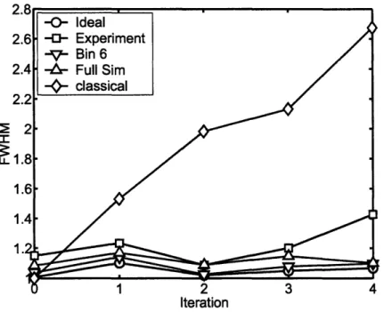
In light of the incoherent variations of localization properties of the map over the en-semble, we wish to select a measure that can be interpreted as the extent to which some portion of the ensemble demonstrates quantum localization. By measuring the full width at half maximum (FWHM) of the probability distribution in successive iterations, we can observe the presence of any dynamical broadening of the distribution, without regard to the background probability offset caused by incoherence, as discussed in Sec. 2.3. Fig. 2-8 shows a plot of the FWHM for each probability distribution plotted in Fig. 2-7. The FWHM data reveals the dynamical properties of the experimentally measured distribution as distinct from the classical behavior. The relative flatness of the experimentally measured FWHM curve through three iterations of the map is consistent with quantum localization in an incoherent ensemble. Numerical simulations show the progression in peak width from the ideal simulation (most narrow) to simulations where decoherence and incoherence are included in the simulation. The numerical simulation which accounts for decoherence but not incoherence corresponds to the momentum distributions plotted in Bin 6 of Fig. 2-6.

2.5

Discussion

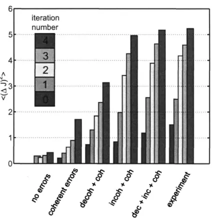
By using numerical simulations to isolate the various types of errors known to influence the experiment, it is possible to measure the relative significance of each type of error by examining the degree to which it leads to delocalization in the system. Figure 2-9 shows the degree to which each type of error causes delocalization in the resulting state, as measured by the second moment of the corresponding probability distribution, thus distinguishing the relative importance of the distinct noise mechanisms in the experiment. The data also

2 2

1.6-

1.4-1 2 3 4

Iteration

Figure 2-8: The full width at half maximum of the momentum distribution after zero through four iterations of the sawtooth map in various implementations: a numerical simu-lation of the exact classical map (diamonds), a numerical simusimu-lation of the exact quantum map (circles), the experimentally implemented map (squares), a numerical simulation of the experimentally implemented map which accounts for decoherence without incoherence (triangles down), a numerical simulation of the experimentally implemented map which accounts for decoherence with incoherence (triangles up). The FWHM reveals that despite the noise affecting the QIP, the distribution mimics the ideal quantum behavior, and does not broaden in a diffusive manner as in the classical case.

5

4

3

V 0A C,9 0 0

Figure 2-9: The second moment of the probability distribution determined from numerical

simulations of the experiment including the error models discussed in the text, compared to

the ideal data and the experimental data. This plot demonstrates the relative importance

of the individual noise mechanisms as they contribute to the experimentally observed

delo-calization process. As more errors are included in numerical simulations, the system shows

stronger delocalization and more closely emulates the experimental data.

iteration

number

1

21

ill

m

...

WMjj

r%

El

F. IF

2 |-

...

...

....

reveals the extent to which the breadth of the distribution is affected by errors in the initial state preparation. Evidently, the coherent errors are essentially inconsequential over at least three iterations of the map. The slope of second moment versus time plot is most strongly affected by incoherent errors, and thus incoherence is determined to be the dominant noise mechanism limiting the degree to which localization is achieved by experimental control, which is consistent with the observations of Sec. 2.3.

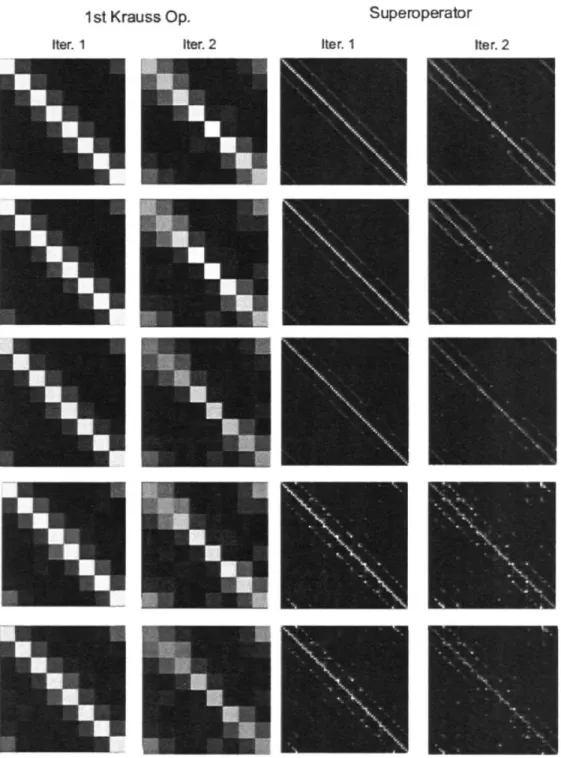
Additional insight on the delocalizing effects of experimental noise and decoherence can be gained by examining the superoperators and the corresponding Kraus operators for each type of numerical simulation. A superoperator of dimension N2 x N2 which describes a completely positive quantum process can be equivalently expressed as an operator sum, which involves at most N Kraus operators of dimension N x N [60]. That is to say that for a general quantum process as in Eq. 2.24,

IPout)

= S Ipin) (2.26)

there is an equivalent representation of the form

Pout =

S

AkpinAtk (2.27)

k

where Ak is the kth Kraus operator, which has a magnitude of Ak

l.

Methods for conversion to and analysis of the Kraus form are given in [47] and [115]. The Kraus form for an ideal implementation of a unitary process would consist of a single Kraus operator which is the corresponding unitary operator describing the process. Therefore, in an implementation where the errors are small, we expect the Kraus operator of largest magnitude to resemble the ideal unitary operator. The numerically simulated superoperators expressed in the momentum basis, along with the largest magnitude Kraus operators, plotted in Fig. 2-10, give a qualitative picture of the differences between a quantum process that leads to localization (in the ideal simulations) and a quantum process that causes some degree of delocalization (in the simulations which include errors). Off-diagonal elements in the unitary or Kraus operator cause transitions between momentum states; diagonal elements alter the magnitude and phase of each momentum state without causing transitions. The qualitative result of the simulated noise is to reduce the bandedness (i.e. the relative magnitude of the

Iter. 1 Iter. 2 Iter. 1 Iter. 2

Figure 2-10: The magnitude of each element of the superoperators and most significant Kraus operators for numerical simulations of the quantum sawtooth map experiment which include different types of errors (top to bottom): (1) no errors, (2) coherent errors, (3) coherent errors and decoherent errors due to relaxation, (4) coherent errors and incoher-ent errors due to rf inhomogeneity, (5) coherincoher-ent, incoherincoher-ent, and decoherincoher-ent errors. The elements are scaled from zero (black) to one (white). The errors in the implementation of the sawtooth map affect the bandedness of each Kraus operator (and similarly of each superoperator).

Superoperator

1 st Krauss Op.

diagonal and near-diagonal elements compared to the off-diagonal elements) of the operator, thus reducing the degree to which a state is localized under the map. The simulated operators for 1 and 2 iterations are progressively less banded as more errors are included in the simulation, which further attests to the sensitivity of localization to experimental noise effects. As explained in Sec. 2.3, Fig. 2-10 again shows qualitatively that rf inhomogeneity has a greater delocalizing effect than decoherence in this implementation of the quantum sawtooth map.

2.6

Conclusions

The quantum sawtooth map has been emulated on a three qubit liquid state nuclear mag-netic resonance quantum information processor in the perturbative localization parameter regime of the map (K = 1.5, L = 7, N = 8). Observing the dynamic behavior of the width of the peak in the momentum probability distribution reveals behavior which is consistent with coherent quantum localization. Due to incoherent noise, this localized peak is superim-posed with a uniform background offset over the probability distribution which represents those parts of the ensemble which are not localized due to local unitary errors which vary over the ensemble.

Numerical simulations of the experiment reveal that the decoherent noise known to act on the system is relatively inconsequential in this implementation of the map, in terms of

its effect on localization when compared with incoherence. This study serves as a test of the capabilities of coherent control and serves to motivate the refinement of our implementation. Specifically, we see that incoherence is the biggest challenge in implementing localization, a highly sensitive quantum coherence-dependent phenomenon. Given the sensitivity of localization to various types and strengths of errors, the degree to which localization can be created and maintained in a QIP serves as a benchmark of practical relevance for assessing the overall degree of coherent control and for identifying which noise mechanisms most significantly reduce the degree of coherent control achieved in the device.