A computer model for tunneling costs,

A COMPUTER MODEL FOR TUNNELING COSTS by

Thomas J. Lamb

S.B., Massachusetts Institute of Technology 1969

Submitted in partial fulfillment of the requirements for the degree of

Master of Science at the

Massachusetts Institute of Technology June 1971

Signature of Author. .. ...

Department of Civil Engineering, May 14, 1971 Certified by . . . . . . . . . . . . . . . . . . . . . . . Thesis Supervisor Accepted by . . . . . . . . . . . . . . . . . . . . . . .

ABSTRACT

A COMPUTER MODEL FOR TUNNELING COSTS by

THOMAS JAMES LAMB

Submitted to the Department of Civil Engineering on May 14, 1971, in partial fulfillment of the requirements for the degree of Master of Science.

Tunnels are being used more and more to solve the press-ing environmental and social problems of our society. They are very expensive, but little is known concerning the

influence of various factors upon the cost. An approach has been developed which uses a computer to model tunnel

con-struction. This model is detailed enough to permit cost estimation, sensitivity analysis, and the evaluation of new construction techniques.

The model consists of four stages: setting up the data, determining the cost of each segment, determining the cost of each reach, and finding the minimum cost. Event simula-tion is used to model the excavasimula-tion process. Simulation or network techniques are used to model particular operations.

Decision C.P.M. is used to find the cost of the reach. The first stage has been implemented on the MULTICS time sharing system at M.I.T. It is written in the PL/1 programming

language.

Thesis Supervisor: Professor Fred Moavenzadeh Associate Professor of Civil Engineering Title:

ACKNOWLEDGEM4ENT

I wish to thank my advisor, Professor Fred Moavenzadeh, for his constant encouragement of this work and much helpful advice. _{Professor Frederick J. McGarry and Professor Ronald} C. _{Hirschfeld of M.I.T. and Mr. Frank Wheby of the Harza} Engineering Company also provided many helpful discussions.

Special thanks is _{due to Christopher Herot who wrote} the programs and whose knowledge of programming was an invaluable aid. Debbie Allinson provided much needed

encouragement and moral support. Rosemary Dujsik typed the thesis quickly and accurately.

Many other persons, too numerous to identify, lent encouragement and provided information, for which I am very grateful.

TABLE OF CONTENTS Title Page Abstract Acknowledgement Table of Contents List of Figures List of Tables Chapter One Introduction Chapter Two

Tunnel Cost Estimation

A. Estimation Procedures

B. Tunnel Estimation Procedures Chapter Three

The Model Framework A. Approach B. Logic C. Framework

D. _{Tunnel Definition Language} E. Conflict Analyzer

F. Physical Quantities Analyzer G. Prescheduler

H. Time Analyzer

I. Scheduler for Segments J. Preliminary Cost Analyzer

Page 1 2 3 4 7 8 9 16 17 18 25 26 28 42 45 46 52 55 55 56 57

K. Conflict Analyzer ₅₈

L. Main Scheduler ₅₉

M. Unit Cost Calculator ₅₉

N. Cost Analyzer ₅₉

O. Cost Minimizer 60

Chapter Four

Conclusions and Discussion ₆₁

References ₆₅

Appendix A

Tunnel Construction ₇₂

Part I: Components of the Tunneling Cycle 73

A. Excavation ₇₃ B. Mucking ₇₄ C. Support ₇₇ D. Lining ₇₉ E. Groundwater Control ₈₁ F. Ventilation ₈₂ G. Surface Plant ₈₃ H. Safety ₈₄

Part II: Tunnel Costs ₈₆

A. Tunnel Cost Components 86

B. Influence of Geology and GroundJater 92

C. The Effect of 'eometry 94

D. The Effect of Excavation Method 97

E. _{The Effect of Mucking Method 98}

F. _{The Effect of Support and Lining Systems 99} 5

G. H. I. Appendix B Tunne 1 A. B. C. D. E. F. G. H. I. Appendix C A Cost A. B. C. Appendix D Prograrr A. B.

The Effect of Groundwater and Ventilation Regional Considerations Time Considerations Definition Language Introduction The Program Users Manual

Initiate-Symtab and Mo dify-Symtab Initiate-Methods and Modify-Methods Initiate-Tunnel and tdl Tunnel Example Listing Estimation Program Description Structure

Output and Listing

for Powder Calculations Example Listing 100 101

102

103

LIST OF FIGURES

Figure 1: Projected Tunneling Activity ₁₁ Figure 2: Cost Increases in Tunnels and Hydroelectric 13

Projects

Figure 3: Excavation Cost vs. Diameter 20

Figure 4: Harza Cost Equation 23

Figure 5: Bledsoe's Approach 24

Figure 6: Network for Reach Construction 30 Figure 7: Model for the Drilling Event 40

Figure 8: Drilling Submodel 41

Figure 9. Logical Setup of Model 43

Figure 10. Flow Chart of Proposed Program 44 Figure 11. Tunnel Definition Language Example 49

LIST OF TABLES

Page

Table 1: D.C.P.M. Operations ₃₁

Table 2: D.C.P.M. Constraints 33

Table 3: Events for the Excavation Simulation 34

Table 4: Drilling Crew 36

Table 5: Events in Simulation for Drilling Crew 37 Table 6: Events in Simulation for Surface Crew 38

Table 7: Construction Methods 47

Table 8: Conflict Criteria 48

CHAPTER ONE In troduc tion

INTRODUCTION

The space beneath our cities can be used for transpor-tation, service, and possibly living space. The interior of the earth has been utilized to a very limited extent for subways, deep basements, and depressed highways, but the potential exists for a much greater utilization of under-ground space. It is expected that efforts to better utilize

this space will be substantially increased during the next several years. The facilities to provide water and power services frequently make use of underground chambers or con-duits, and will do so even more in the future, to avoid

surface congestion.

Several studies have been made in an attempt to pre-dict future tunneling activity. Figure 1 shows the results of two such studies, one by the Committee on Rapid Excavation of the National Research Council (1968) and one by the U.S. delegation to the Organization for Economic Cooperation and Development (1970). The two studies indicate a growth in demand of more than 100% every ten years, but the absolute predicted demand, in dollars, varies widely. This figure

indicates that demand will be large, will grow rapidly, and is extrodinarily difficult to predict. In another study, Operations Research, Inc. (Lago et al, 1967) indicated that the demand for tunnels is a function of their cost.

Even if demand could be predicted, the costs associ-ated with these tunnels would not be well known. They cannot

OECD

rYOU-CW;( T~-L~ L '-CI

~

~C

~--.-

0-1970-1980

OECD

FIGURE

I

PROJECT

ED

-5

.4

,~,,

TUNNELING

ACTIVITY

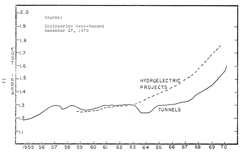
be extrapolated using a

cost

index such as that given in

Engineering News-Record.

Figure 2 shows past costs of tunnels

and of hydroelectric projects, which are more or less typical

of heavy construction. Tunnel costs seem at present to be

increasing less rapidly than costs for heavy construction

in general.

If this trend continues, tunneling will become

more and more attractive when compared with surface

construc-tion.

The use of a cost index implies a base cost to which

the index can be applied, and this cost must be estimated.

Until very recently, satisfactory methods for predicting

the cost of a tunnel quickly and accurately did not exist,

and producing the base estimate was a major task. Even very careful estimates, such as a contractors bidding estimate, or the engineers estimate, frequently disagree with each other and with the final cost. There are two major reasons for this. The cost of a tunnel is highly dependent upon the geologic conditions encountered, and geologic conditions are rarely well known. It is desirable to estimate the cost of a tunnel for several geologies, so that a range of costs is available and construction strategies for use in emergencies can be worked out, but this is rarely done, because of the

time required to make accurate estimates.

The second reason for the inaccuracy of tunnel cost estimates in the dependence of cost upon the method used and upon the interactions between the operations occuring

under-2.0

Source:

December

17,

1970

C/

0 1.7

"

T

_1.6

N

HYDROELECTRIC

E

PROJECTS

,

X 1.

...

_TUNNELS

1955

56

57

58

59

60

61

62

63

64

65

66

67

68

69

70

2

COST INCREASES

IN

TUNNELS

ground. The various components of a tunnel (excavation, muck-ing, support, etc.) are usually given separate costs, but

this is somewhat misleading, since they are really inter-dependent. Alternate construction methods are rarely inves-tigated in detail, and the simplified estimating procedures that are used to investigate alternatives can be inaccurate. Appendix A discusses the tunneling process and the factors which influence cost.

Considerable work is being done in an attempt to deter-mine geologic conditions with more accuracy. Research is also in progress evaluating new construction methods. Some procedure is needed to evaluate these new methods of exca-vation with respect to cost. Also, an improved method of estimating costs is needed, so that costs can be determined more rapidly and with greater accuracy. A computer program which can estimate costs in great detail for various con-struction methods fits these requirements. The program should take into account what is happening underground

minute by minute. The large number of calculations necessary can be done quickly and accurately, so more alternatives

can be investigated.

It is the purpose of this thesis to develop the logic for such a program. A complete implementation of the

detailed approach outlined herein is beyond the scope of this work, but a considerably more limited version, which illustrates the basic approach taken, has been implemented.

Suggestions are presented for the complete implementation, but the details are lacking. The program has been written in PL/1 on the MULTICS system (time sharing) at M.I.T. This

language and system were used because of the relative ease with which they can handle large quantities of data.

CHAPTER TWO Tunnel Cost Estimation

TUNNEL COST ESTIMATION

Estimation Procedures

There are several methods of cost estimation currently in use, and probably as many variations as there are estima-tors. Three basic approaches will be discussed below. Each has its advantages and disadvantages, and which is the "best" depends upon the purpose for which the estimate is made.

Costs are sometimes collected from previous projects and used as a basis for predicting future costs, often

coupled with a cost index. In order for the estimate to be reasonable, the project to be estimated must closely match the projects from which data is obtained, both i.n design and in construction procedure. This type of estimate is fairly simple to make and does not require a detailed knowledge of design or construction on the part of the estimator. Thus, it is useful for preliminary planning. It is easy for an estimate of this type to be misleading, however, especially if significantly different construction techniques are used.

The second type of estimate is based upon unit costs. These can be either calculated, based upon the operations necessary to do the job, or they can be based on costs from previous jobs. This type of es-timate requires more knowledge

of design and construction than the previous type, and takes longer to do, but it is more detailed and more reliable. The so-called "law of averages" usually insures that even if the exact construction or design details are not known, the

total cost will be reasonable. This is the type of estimate used most often in feasibility studies. The reliability of this type of estimate is quite variable, depending upon how the unit costs are obtained.

The third type of estimate is a very detailed calculation based upon the exact knowledge of how an operation is to be

performed, who is to do it, how long it will take, and the labor, equipment, and material prices. This type of esti-mate requires a detailed knowledge of the project design and elaborate preplanning of the work. Hence, it is a difficult and time consuming type of estimate to make. On the other hand, it is probably the most reliable estimate possible. The basic cost data (wages and equipment and material prices) are fairly easy to obtain, but productivity of men and

machines is difficult to evaluate. New techniques can be incorporated into the estimate if their characteristics are known. Deathridge (1965) and Parker (1970) give excellent treatments of this type of estimate.

Contractors often use this type of estimate on big jobs, since it is rather easy to adapt to C.P.M. or PERT scheduling techniques. This method has the additional advantage of

specifying the details of each operation, so that if costs are excessive, the operations departing from assumptions can be pinpointed and perhaps rectified.

Tunnel Estimation Procedures

the estimation of tunnel costs was puiblished by the California Department of Water Resources (1959). The Department was

concerned with various alternative aqueduct systems to serve southern California, and they developed a systematic cost estimation procedure for planning purposes.

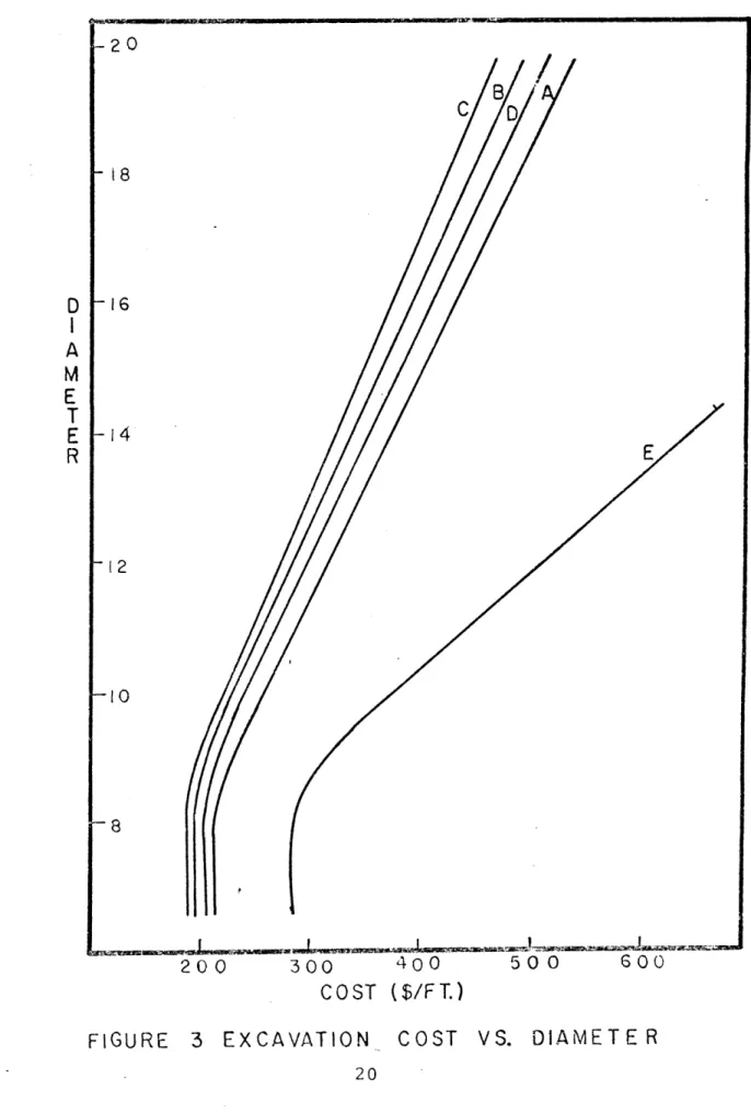
Using tunnel diameter and geologic conditions as their basic variables, the Department evaluated many previous

tunnel jobs and constructed charts giving the costs of the various components versus these variables. These charts provide a quick and fairly accurate estimate of the cost of constructing a non-pressure water tunnel in California

in 1957. This procedure is a vast improvement over a completely separate estimate for each tunnel. It is also

instructive to see graphically how various factors influence cost. Figure 3 shows one of their charts, plotting cost vs. diameter for various geologies.

The procedure developed in California has many draw-backs which make it difficult to use in general. It gives accurate results only for a specific area of the U.S. at a specific time. Hirschfeld (1965) has updated the costs in this report to 1964 using the Engineering News-Record Cost Index, but the applicability of this Index to tuninels is somewhat questionable, and no provision is made for costs

in different regions of the country. It may well be easier to derive new cost curves than to compute an accurate cost index.

20

B

CD

18

D

-16

A

M

E

T

E

-14

R

E

12

10

8

200

300

400

500

600

COST (S/FT.)

FIGURE

3 EXCAVATION

COST VS. DIAMETER

The California method takes account only of drilled and blasted tunnels, driven from portals. Extensive

additional computations are required if tunneling machines are used or if the tunnel is driven from a shaft. Also, the design of the supports and lining and the advance rates are fixed, and there is no easy way to incorporate different designs into the charts. In spite of these drawbacks, the California charts are useful in obtaining a first approx-imation of tunnel costs, if care is taken in projecting prices to today's levels.

More recently, (1968, 1970) the Harza Engineering Company has developed cost estimation procedures for the U.S. Department of Transportation. The aim of these studies was to provide cost estimates for the tunnels in a high

speed rail transportation system in the Northeast Corridor. Their first effort, (March, 1968) was set up much like the California estimation procedure, except that the breakdown into components was a bit different and tunneling machines were considered. Their geological classification system is difficult to use and the tunnel design is fixed. The prices given are for Chicago in 1967, and no criteria are given for modification for different times and places.

The second effort of this company utilized a computer to estimate the costs. The computer program is considerably more flexible than the previous procedure, and various

combinations of excavation, mucking, support, and lining

methods can be evaluated. The geological classification

system is much better, and attempts have been made to extend the estimates to other parts of the country.

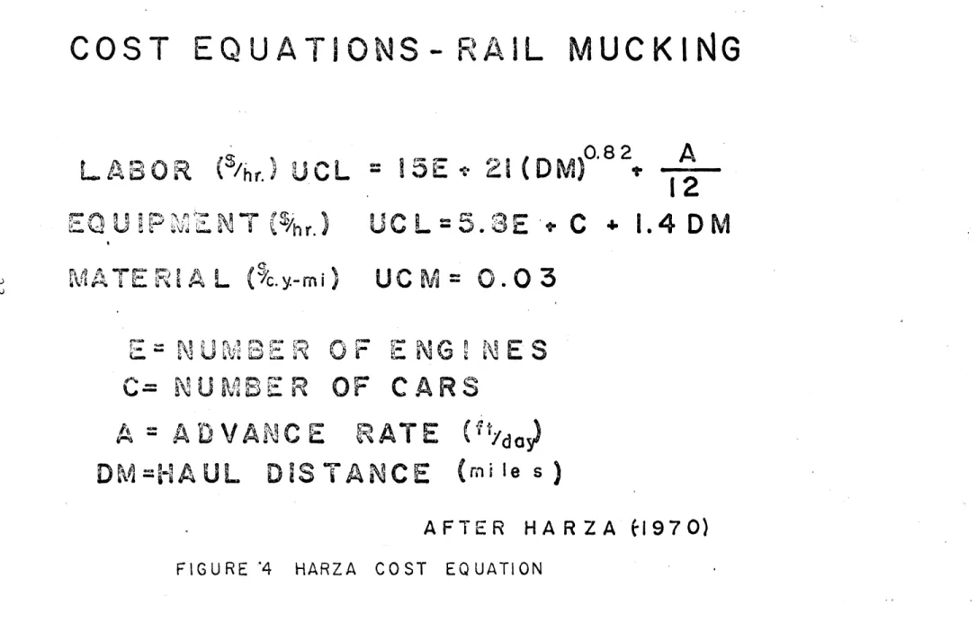
The equations which the computer uses to estimate costs (see Figure 4) were derived by estimating costs for various cases (in detail), deciding what factors influence the cost, and plotting these costs versus the factors to obtain a cost equation. The design details are built in, as are the

details of all construction procedures. Nevertheless, this program represents a great improvement over previous pro-cedures.

There are many other cost estimation procedures used by individuals and agencies which have not been published. It is probably safe to say that each estimator has his own more or less systematic procedure. These procedures are usually quite detailed, cumbersome, and difficult to ex-plain. Bledsoe (1970) suggests that a much better approach would be to calculate the cost of a tunnel by knowing what is happening at the face in great detail and using a computer to calculate the cost directly. This "model" of underground construction could then be modified, and the effect upon cost noted.

Bledsoe's procedure is outlined in Figure 5. The

approach suggested in the next chapter is similar to Bledsoe's approach in that both consider the tunneling operation in great detail, but the techniques used are quite different.

COST EQUATIONS- RAIL MUCKING

LABOR

(S/hr.) UCL

=

15E

0.

82

A

21(DM)

₁₂

12

E0,4U

'!P

Ago".

MATE iA L

('c..-mi)

UCL=5.3E

-UCM= 0.03

C * I.4DM

C= NiUMER

A = ADVAACE

N ES

OF CARS

RATE

_("t/do

DM=HAUL

DISTANCE

(mile

s

)

AFTER HARZA

FIGURE

A4

HARZA

COST

EQUATION

CHAPTER THREE The Model Framework

Tunnel construction today is largely a trial and error process. Very little analysis of the actual construction process has been performed, the excuse usually being that geology is too variable. A computer program capable of analyzing construction should be fast enough to calculate results for various geologic conditions and overcome this difficulty. The framework for such a model is presented in this chapter. The goals of such a program are first dis-cussed and the approach taken to meet these goals is out-lined. The logic of the program and the method of analysis is then described. Finally, a framework for implementation and partial results are presented.

Approach

Three goals should be met by the program:

1) Accurate Cost Estimation.

2) The ability to perform sensitivity analysis and to evaluate new construction methods. 3) Convenience and ease of use.

These goals determined the approach taken.

Cost estimates which are reasonably accurate can be obtained by using COHART (the program developed by Harza Engineering) or the modification of this program presented in Appendix B. If construction cost is all that is desired, and if current methods are to be used, it is not necessary to use a more detailed program. A detailed program will

give accurate cost estimates also, but improvement will be marginal.

A detailed approach is necessary for sensitivity analy-sis. It is impossible to determine the effect of, for

example, drilling crew size upon cost unless the effect of a change in drilling time upon the mucking or support

operations can be specified. The relation is not simple, because crews must be transported to the face, work areas are crowded and operations interfere, and there are many alternate ways of scheduling the operations underground. It is extremely simplistic to look at tunnel construction as a collection of independent events, and any sensitivity analysis based upon this assumption may be misleading. Miuch the same thing can be said for the evaluation of a new

construction technique; interactions cannot be ignored. A detailed approach has the advantage that the cost information required (wages, equipment operating costs, and material costs) is much easier to obtain than the cost per foot for some operation. Cost per foot depends upon geology, geometry, method used, schedule, equipment, etc., and the relationship is anything but clear. (It should be noted that a cost model capable of sensitivity analysis can help clarify these relationships).

Defining exactly what is happening during construction is very difficult because activities vary from tunnel to tunnel. The construction details are set by the contractor based

largely upon his feeling for what is most effective. A de-tailed program must either contain assumptions as to the

schedule of allow the user to specify it. The most convenient way for a user to specify the schedule is through the use of

time sharing. With this type of system, the user can inter-act with the model and modify his assumptions based upon results.

The amount of time a given operation takes is not well defined. It is possible to derive time distributions for certain operations, either based upon past data or assumed, and use simulation to determine the time for the entire

process. Simulation can also be used when productivities or efficiencies are not known exactly

A detailed program should model the tunnel construction process operation by operation, determining progress, the amount of time each man works, and the amount of time each piece of equipment is in operation. A full day (three shifts) must be modeled to take care of variations in scheduling and transportation. The user must define how things are to be done. Logic

Tunnel construction must be analyzed at three levels of detail. The reach level is the most general level. A reach is that portion of the tunnel excavated from one shaft or portal (c.f., Harza, 1970). The cost of the reach includes the cost of tunnel construction, the cost of the plant and surface equipment, the cost of the shaft or portal, and

overhead, profit, and interest. The reach can be modeled

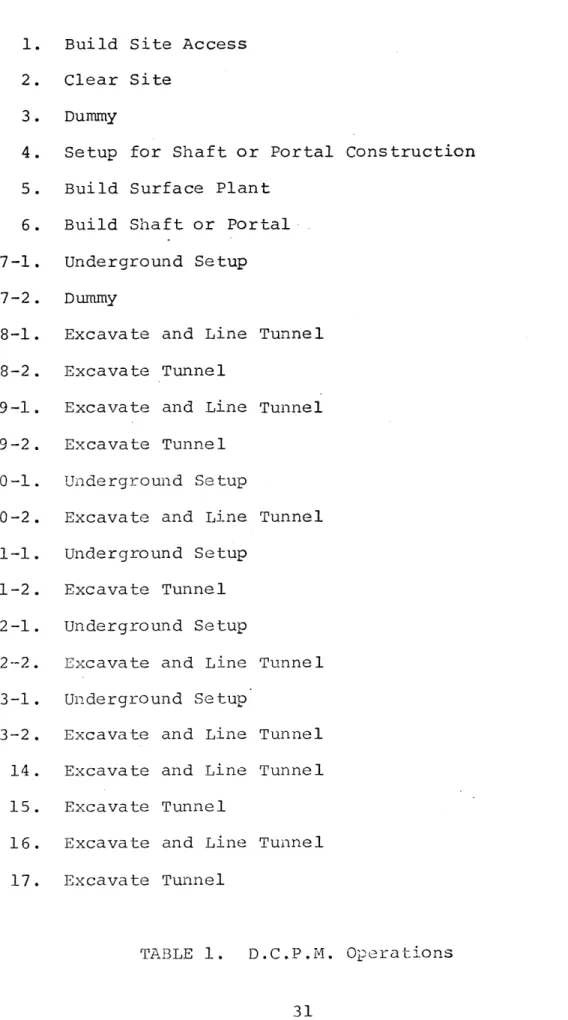
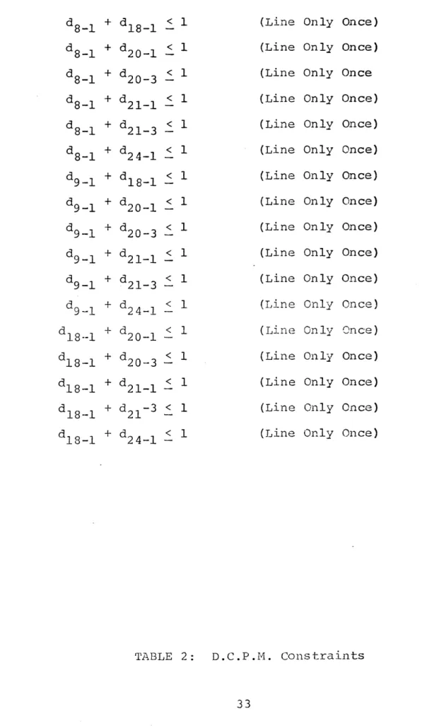
using a decision C.P.M. network as shown in Figure 6. Table 1 lists the operations and Table 2 lists the constraints.

This network can be solved using integer linear programming (Crowston & Thompson, 1965).

Costs and times for each reach operation can be determined by modeling it. Clearing operations, shaft construction,

and finishing operations will not be considered further, but they could be modeled in a manner similar to excavation. The determination of excavation cost requires that the seg-ments within the reach be modeled.

A segment is a portion of the tunnel in which every-thing is constant. After a certain number of segments have been constructed, some of the plant may be moved underground.

If the cost of construction is computed both with the move and without the move, the D.C.P.M. reach network will tell which is the best solution.

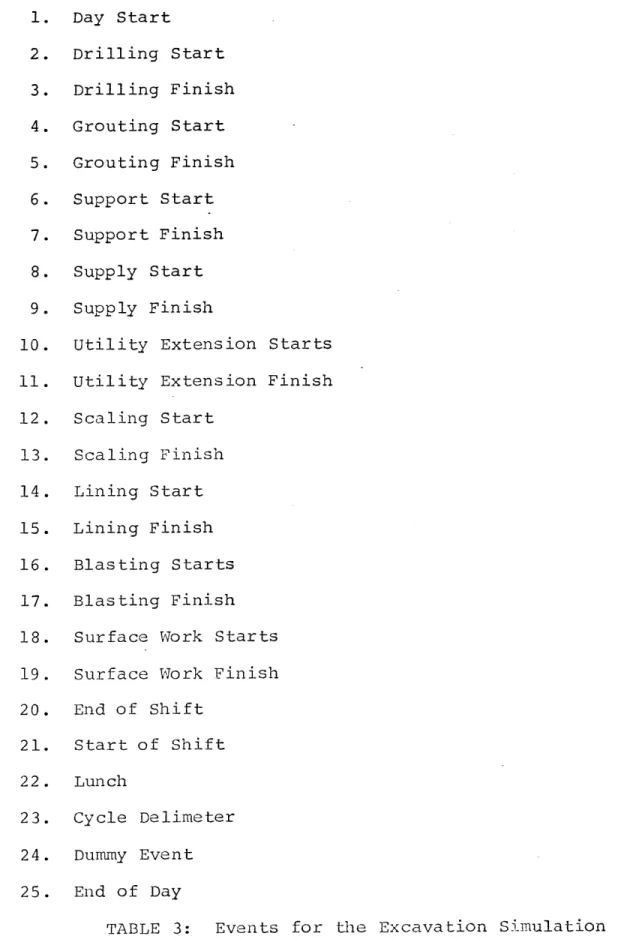
Segment construction can be modeled using event simula-tion. Several time periods are of interest. The cycle is basic to tunneling and must be kept in mind. A shift must be modeled in order to determine transportation costs. A day, or three shifts, may have to be modeled, depending upon scheduling. Table 3 lists the events which might be used in a simulation of excavation. The events can be ordered by

the user. Defining the sequence of events will determine the schedule underground.

1. Build Site Access 2. Clear Site

3. Dummy

4. Setup for Shaft or Portal Construction 5. Build Surface Plant

6. Build Shaft or Portal 7-1. Underground Setup 7-2. Dummy

8-1. Excavate and Line Tunnel 8-2. Excavate Tunnel

9-1. Excavate and Line Tunnel 9-2. Excavate Tunnel

10-1. Underground Setup

10-2. Excavate and Line Tunnel 11-1. Underground Setup

11-2. Excavate Tunnel 12-1. Underground Setup

12-2. Excavate and Line Tunnel 13-1. Underground Setup

13-2. Excavate and Line Tunnel 14. Excavate and Line Tunnel 15. Excavate Tunnel

16. Excavate and Line Tunnel 17. Excavate Tunnel

18-1. Line Tunnel 18-2. Dummy

19-1. Cleanup

19-2. Finish Shaft or Portal 19-3. Dummy

20-1. Finish Shaft or Portal 20-2. Finish Shaft or Portal 20-3. Line Tunnel

21-1. Line Tunnel 21-2. Cleanup 21-3. Cleanup

22. Finish Shaft or Portal 23. Cleanup

24-1. Line Tunnel 24-2. Dummy

25. Line Tunnel

26. Finish Shaft or Portal 27. Cleanup

28. Line Tunnel 29. Final Cleanup

d8-1 + d18-1 < 1 (Line Only Once) d8- 1 + d20-1 < 1 (Line Only Once)

d8-1 + d20-3 < 1 (Line Only Once d8-1 + d21-1 < 1 (Line Only Once) d8-1 + d21-3 < 1 (Line Only Once) d8- 1 + d24-1 < 1 (Line Only Once)

d + d < 1 (Line Only Once) 98-1 201-3

-d9-

+ d21-1 < 1

(Line Only Once)

d + d < 1 (Line Only Once)

9-1 21-3

d _9-1 + d _{+ d218-1} < 1 (Line Only Once)_{(Line Only Once)}

dl8-

+ d20_l < 1

(Line Only Once)

d + d < 1 (Line Only Once)

18-1 20-1 < 1 (Line Only Once) d 181 + d 21-3 < 1 (Line Only Once) d 8-1 + d 24-1 < 1 (Line Only Once)

TABLE 2: D.C.P.M. Constraints TABLE 2: D.C.P.1. Constraints

1. Day Start 2. Drilling Start 3. Drilling Finish 4. Grouting Start 5. Grouting Finish 6. Support Start 7. Support Finish 8. Supply Start 9. Supply Finish

10. Utility Extension Starts 11. Utility Extension Finish 12. Scaling Start 13. Scaling Finish 14. Lining Start 15. Lining Finish 16. Blasting Starts 17. Blasting Finish 18. Surface Work Starts 19. Surface Work Finish 20. End of Shift 21. Start of Shift 22. Lunch 23. Cycle Delimeter 24. Dummy Event 25. End of Day

Each event in Table 3 represents the start or comple-tion of an operacomple-tion. Each operation can in turn be modeled by a simulation, and the time of occurrence of the start of the next operation or the finish of the operation in question can be determined. The solution of the main simulation will give construction time. (Cost is determined by the operation simulations). The schedule can be changed and the simula-tion run again to determine the sensitivity of cost and completion time to scheduling.

Interactions between operations can be modeled by inter-actions among the operations simulations. For this purpose, and for cost computations, the groups of men performing

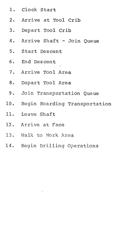
different operations must be separated. Crews can be defined for this purpose. Table 4 lists the members of the drilling crew. The user must specify the size and composition of each crew and their wages. The actions of each crew can be simulated separately, with the simulations interacting. An example will clarify this.

The day start event will initiate the two sequences of events listed in Tables 5 and 6. (Additional simulations will be initiated for the other crews). The drilling crew cannot descend the shaft until the surface crew has readied the hoist. There may be additional interactions with other crews. The user must specify these relationships. Simula-tion languages such as SIMSCRIPT II make this relatively easy.

1 Foreman N Drillers N Helpers 1 Supply Man

NOTE: Crew Size must be Defined by the User

1. Clock Start

2. Arrive at Tool Crib 3. Depart Tool Crib

4. Arrive Shaft - Join Queue 5. Start Descent

6. End Descent

7. Arrive Tool Area 8. Depart Tool Area

9. _{Join Transportation Queue} 10. Begin Boarding Transportation 11. Leave Shaft

12. Arrive at Face 13. Walk to Work Area

14. Begin Drilling Operations

Clock Start Open Crib

Hoist Ready

Ventilation System Started Compressors Started

Generators Started

Begin Readying Muck Disposal System Begin Startup of Concrete Batch Plant Begin Surface Operation Model

Each event in Tables 5 and 6 can be modeled in as much detail as desired. _{Sufficient accuracy can probably be} obtained by simply specifying a time distribution for each event. Costs for the men can be determined by multiplying

times by wages. _{Time can be further broken down into} produc-tive time and lost time if desired. The equipment usage time can also be collected and equipment cost calculated.

Event 14 in Table 5 triggers the start of the drilling event in Table 3. If actual drilling is uneffected by

other events, techniques more efficient than simulation can be used. Figure 7 shows a GERT (Graphical Evaluation and

Review Technique, Pritsker, 1966) network which can be used to simulate drilling. Programs exist for the solution of GERT networks. The solution of this network will give the time and cost for drilling. For each branch, crew wages and equipment operating costs must be specified. Material

cost (bits and power) can be computed separately. The

probability of completing the drilling on schedule can also be obtained from the GERT network.

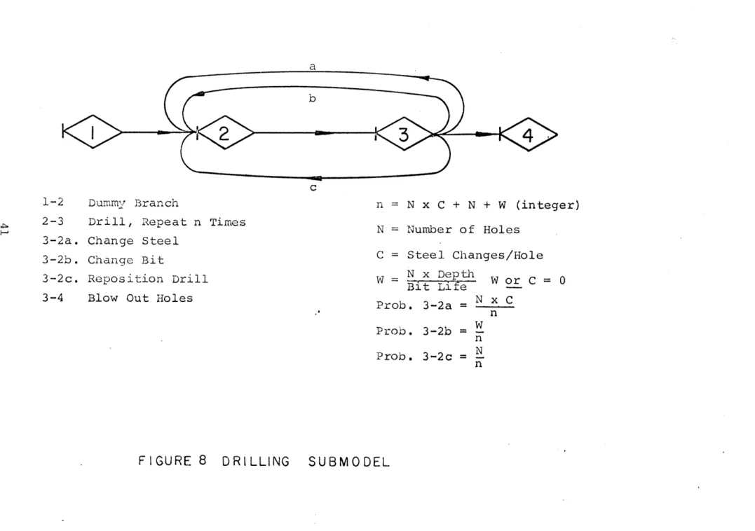
It may be desirable to model certain branches of this network in more detail. Figure 8 shows a submodel for the drill branch. This GERT network can be solved for the time and cost of actual drilling. The user must specify time and cost information for each branch and must supply the parameters used to determine n.

Advance Sliding Floor Lay Track Bring up Drills Bring up Jumbo Bring up Jumbo Dummy Branch Bring up Drills Dummy Branch Position Jumbo Position Drills Connect Utilities Drill Disconnect Utilities

One Branch Chosen by User

One Branch Chosen by User

One Branch Chosen by User

MIODEL

FOR THE DRILLING EVENT

6-7

7-8

FIGURE 7

Dummy Branch

2-3 Drill, Repeat n Times

3-2a. Change Steel 3-2b. Change Bit

3-2c. Reposition Drill

3-4 Blow Out Holes

n = N x C + N + W (integer)

N = Number of Holes

C = Steel Changes/Hole W = N x Depth -_Bit ... ._Lifet --- , , W or C -- 0

Prob. 3-2a Nx C n Prob. 32b -n Prob. 3-2c = n

FIGURE

8

DRILLING

SUBMODEL

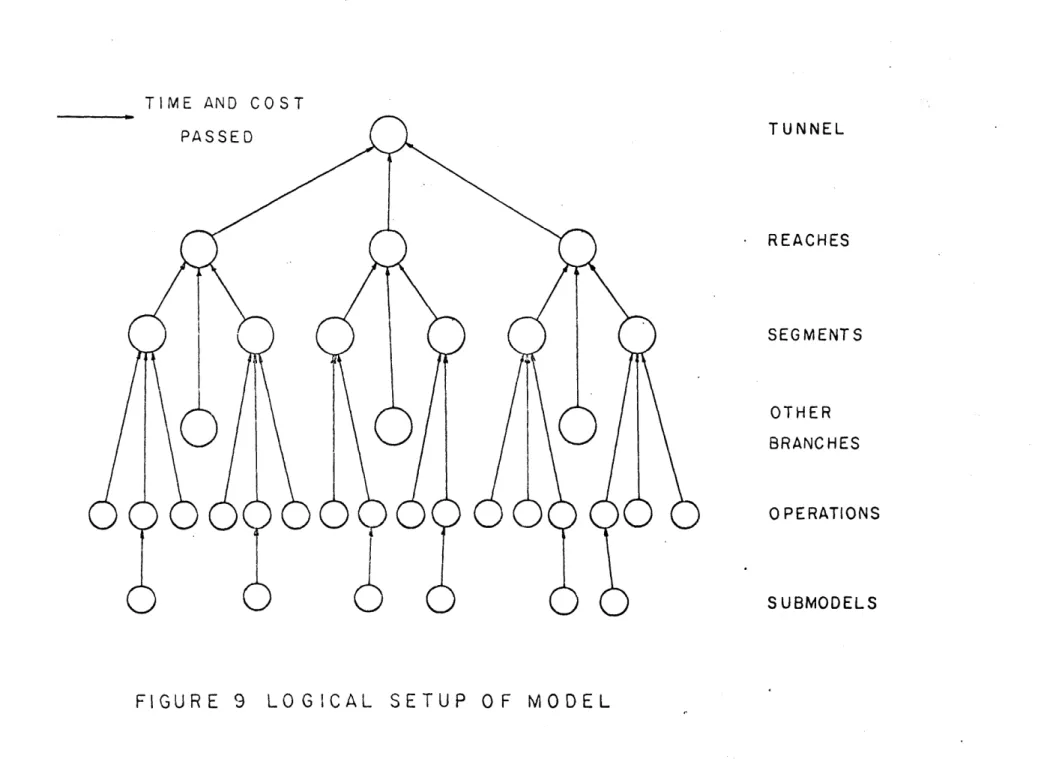
with it. Where interactions can be ignored, efficient com-putational methods such as GERT can be used. Where events interact, event simulation is probably a better procedure. Interactions and sequences must be defined by the user. Once the main simulation of excavation has been constructed it should be run several times to obtain a reasonable cost-advance relationship. The simulations can be constructed to reflect delays due to unexpected geologic conditions or equipment breakdowns by adding a breakdown or delay event and specifying its interactions with other events. In

addition, more detail can be added to the analysis. Running time on the computer may be a limitation in this respect. Figure 9 summarizes the logic for tunnel construction modeling. Several reach models can be combined to form a model for the entire tunnel, as shown here.

The Framework

A framework for the implementation of the model has been developed and is shown in Figure 10. Four stages are used: defining the tunnel, modeling segment construction, and cost minimization.

The first stage consists of the tunnel definition language and the conflict analyzer. These two processors define the geologic and geometric properties of the tunnel and the construction methods to be used. The tunnel

definition language has been implemented on the Multics time sharing system at M.I.T. It is written in the PL/l

TIME AND COST

TUNNEL

REACHES

SEGMENTS

OTHER

BRANCHES

OPERATIONS

SUBMODELS

METO0 S

LL

U

Ue

TUNNEL~

0OFLC

0HSCLTM

REACH

EQUIPMENT

CONSTRUCTION

COST AND

DESCRIPTION

DEPRECIATION

D ATA

PLANT AND

OVERHEAD

UNIT COST

SETUP

EQUIPMENT

PROFIT

DATA

_TIMES

_DEFINITIONS

_EXTERNALS

RETURN

PRELIMINARY

FOR

CONFLICT

MAIN

UNIT

COST

COST

COST

NEXT METHOD

ANALYZER

SCHEDULER

CALCULATOR

_ANALYZER

ANALYZER

OR NEXT

SEGMENT

iEDULE

COST

FOR

METIH )DS UO ED

WCRK SCHEDULE

Cos

N E W' J N I

EACH

EACH METHOD

_{I % E AC H}

_{I N}

_REACH

_{COSTS FOR}

_{f:O f}

.THOD

_AND

SEGMENT OF

_{FOR EACH}

E Q U I PM E N T

_{C 0 M H I}

3M E N T

EACH SEGMENT

A REACH

COMBINATION

0 F %l

E

programming language. A listing and users manual is pre-sented in Appendix C.

Tunnel Definition Language

The tunnel definition language consists of 6 programs: initiate-tunnel, initiate-symtab, initiate-methods, modify-methods, modify-symtab, and tdl. Initiate-tunnel names the tunnel, defines the maximum number of reaches, shafts, and segments in the tunnel, and sets up a data structure to hold geologic, geometric, and method data for each segment. tdl can be called either automatically by initiate-tunnel or, if the information about an existing tunnel is to be changed, directly by the user. tdl asks for the shaft where each reach originates and its destination shaft. It also requests names for the segments in each reach and geologic and

geometric information for each segment. The number of shafts, reaches, and segments named in tdl can be less than the

number specified in initiate-tunnel.

Initiate-symtab tells the computer where the symbol table is. The symbol table contains the names given to each item of geologic and geometric data and its location in the array where it is stored. Modify-symtab can be used to add or delete names.

Initiate-methods identifies a table of methods to the computer. The user can then describe what construction methods he wants to consider through the use of modify-methods. Methods which might be considered are listed in

Table 7. Initiate-methods also identifies a table of

criteria used by the conflict analyzer to eliminate methods. Table 8 lists some sample criteria. Modify-methods can be used to add, delete, of change criteria. Figure 11 shows an example of the use of the tunnel definition language. For more details, refer to Appendix C.

The geologic information needed is R.Q.D. (see Deere et al, 1969), rock compressive strength (psi), initial

groundwater inflow (gallons per minute at the face), steady state groundwater inflow (g.p.m./foot), and rock temperature. R.Q.D. or rock strength may be specified as a probability distribution with a given mean and standard deviation. The geologic information must be obtained from a geologic

exploration of the tunnel site. Great accuracy cannot be expected.

Geometric information required is tunnel size and shape, slope, depth, and length. These parameters are determined by the tunnel design. The size and shape are specified by a radius and center co-ordinate for circular tunnels and by four co-ordinates and four radii for non-circular tunnels. Refer to Figure 12. A radius of zero indicates a flat surface. The size specified is finished size. The use of this type of specification permits any size or shape of tunnel to be analyzed.

Conflict Analyzer

Excavation Methods

Drill and Blast--Conventional Heading and Bench

Multiple Drift Mechanical Mole Support Methods Steel Supports Rock Bolts Shotcrete or Gunnite None Grouting Methods Pregrouting Chemical Concrete Grouting Chemical Concrete Pumping Pumps No Pumps Lining Methods None Concrete Sho tcre te Mucking Methods Electric Train Diesel Train Electric Truck Diesel Truck Belt Conveyor

I. Geology

if strength > 32,000 psi, mole eliminated if RQD < 90, some support necessary

if RQD < 25, steel sets necessary II. Groundwater

if sustained inflow > 15 gpm, mole eliminated

if sustained inflow > 0, some grouting or pumping neeed if sustained inflow > 100 gpm, grouting needed

if sustained inflow > 500 gpm, pumps needed also if initial inflow < 1000 gpm, no pregrouting if initial inflow > 50 gpm, mole eliminated if sustained (after grouting) > 5 gpm, lining must be used

III. Geometry

if shape not circular, mole eliminated

if diameter 15', truck mucking eliminated IV. Method

if drill and blast used, no conveyor mucking if pregrouting used, eliminate mole

V. Combinations

if RQD > 50, and if diameter < 15', eliminate heading and bench

if ROD > 25, and if diameter < 15', eliminate multiple drift

if RQD < 95, and if no lining used, support must be used

if RQD < 95, and if no support used, lining must be used

if inflow (sustained) > 25 gpm, and if RQD < 50, grouting required

tunnel test

syritab

found

pdb

found

new tunnel

how many

reaches? 2

how many

shafts?

3

how

many

segments? 4

TUL

specify components:

reach

shaft1

A

porl

shaft2

ss

sss

segments

ab

cd

FIGURE

II

TUNNEL DEFINITION

(SEE

APPENDIX

B

FOR

LANGUAGE EXAMPLE

S---depth 3000. init_gwat_ inflow 0.0 sustained gwat_ i 0.0 rock_tremp 50.0 shape 2 rm: sup rb lt shot ;i1: gap none

>rch A

r.m: exc dab mole m: ruck rail trck r: ilin none

iq

r 2122 11.484 50G+234

X

F IGURE 12

X2 ,Y'

methods which cannot be used because of geologic or geo-metric conditions. The purpose of the conflict analyzer is to reduce the number of computations required. If all

possible combinations of the methods listed in Table 7 were used, almost 2000 cases would have to be considered. This would lead to the use of incredible amounts of computer time.

The conflict analyzer applied criteria similar to those in Table 8 and can reduce substantially the number of cases considered. After the program has been used for a while, the criteria can be made more restrictive and computations further reduced. These changes would be based upon the program results. The conflict analyser has not been

implemented, but it is a fairly simple program.

The second stage of the analysis, the analysis of seg-ments, consists of the physical quantities analyzer, the prescheduler, the time analyzer, the scheduler for segments, and the preliminary cost analyzer with their associated data. This stage designs the tunnel, sets up the construction sche-dule in each segment, and computes the cost of the segment. Physical Quantities Analyzer

The physical quantities analyzer designs the support and lining system for the tunnel, calculates the amount of powder and number of holes needed (if drill and blast

excavation is used), calculates overbreak and quantity of muck, and computes the amount of concrete and steel needed

analysis is presented below, but more sophisticated tech-niques would require more computer time and the improvement

in design to be gained is dubious.

Deere's criteria can be used for design of support and lining (Deere et al, 1969). These criteria give support spacing and weight and lining thickness as a function of R.Q.D. The criteria will be stored in the table of design parameters. Criteria other than Deere's can be used, if it seems desirable. These criteria will be stored in much the same way as the criteria for the conflict analyzer. The physical quantities analyzer will determine spacing and

thickness. Weight can then be computed from geometry. A program has been written to perform powder calcula-tions for blasting, based upon the results of Langefors and Kihlstr6m (1963). This program, presented in Appendix D, determines the length of holes, number of holes, size of

holes, stemming, degree of packing, and quantity of explosive. Some of these parameters, in addition to area and advance

per round, must be specified and the program will compute the others. The physical quantities analyzer can use this program to determine quantities of explosive, primers, and caps. It should be used twice, once for the cut and once for the rest of the face.

The area of the tunnel is equal to

+ R3 (03 -sin 03) + R4 (04-sin 04) ) where D -1 n

On

2 sin

Dn = length of chord n (D1 = [(X 3 -X1) 2 (Y-Y3) 2 1/2

Refer to Figure 12. An effective radius can now be computed and the tunnel calculations performed as if the tunnel were

circular.

Reff = (AREA/7) 1/2

This analysis assumes that the area/effective radius ratio does not change as tunnel size is increased. While not strictly true, this approximation is fairly accurate

for small size changes.

Excavated diameter can be computed once the lining thickness is known.

Dexc = 2(lining thickness + Reff)

True excavated diameter must include overbreak

D ext _ext D _ex(1 + O.B.)

where

O.B. = % overbreak/100

the quantity of muck produced can be expressed as: (D ext2/4) (1 + B.F.)_ext

where B.F. is the bulking factor. It may be desirable to make O.B. and B.F. random variables.

Pres cheduler

The prescheduler sets up the construction sequence in the segment for a given construction method. The method procedure table contains lists of events similar to those

in Table 3 for each construction method. The user must specify the order of the events. The construction descrip-tion input is used to indicate user interacdescrip-tion with the program.

The events in the method procedure table can be identi-fied by refering to the references on tunnel construction. The main events for mole excavation are the same as those in Table 3, but the subevents are quite different. The main events must have linkages to the approximate sub simu-lations for each method. These linkages can be programmed by using pointers.

Time Analyzer

The time analyzer is responsible for assigning times to the events in _{the lower level simulations, or to the} branches of the lower level networks. These networks or simulations are linked to the main events as mentioned above. A few times can be specified as constant, such as "smoke time" or lunch time. Others must be computed. The construc-tion data base contains the informaconstruc-tion needed to compute these times, such as drill penetration rate or equipment

productivity. The user must specify how much and what type of equipment is to be used. With this information and the output of the physical quantities analyzer, times can be assigned to the simulations. In many cases, a time distri-bution rather than a single time should be used. The user must also specify crew size and composition.

The computation of times is relatively straightforward. The time required to descend the shaft, for example, can be computed from shaft depth and hoist speed:

Time (sec) = Depth (Ft) Speed (f.p.s.)

The constants (or distributions) required for the calcula-tions can be obtained from equipment manufacturers. The California Department of Water Resources and the U.S. Bureau of Reclamation also have large stores of data. The con-struction data base and the table of standard times should have values in them. The user can change these values if he prefers his own or wishes to check sensitivity. The

user must also tell which branches, in the case of networks, are to be deleted.

Scheduler for Segments

The entire simulation is set up and times assigned for all events by the time analyzer. The scheduler defines

interactions and solves the simulation. The user must

define the way events interact, as mentioned in the section on logic. Some knowledge of tunnel construction is required

do this. This knowledge can be gained from the references. Many of the relationships are based on common sense.

After interactions have been specified, the segment simu-lation can be solved. Each crew's time is kept in an account, and can be separated into productive time, travel time, and lost time. Equipment operating time is also noted. The simulations must be written to collect these figures. The entire simulation should be run several times so that cost time curves can be developed for use in the reach D.C.P.M. network.

Preliminary Cost Analyzer

The cost analyzer determines the cost of constructing the segment using a given method. The times collected when the segment simulation is solved are multiplied by unit costs and summed to give total cost.

Crew cost is determined by adding up the wage rates of the members of the crew. These wage rates can be obtained from the U.S. Department of Labor. Provision must be made to pay overtime rates for hours worked in excess of 8 (or some other number).

Equipment operating cost is somewhat more difficult to obtain. Some information can be obtained from manufactures or public agencies. Contractors are the best source of

such data, but they are usually reluctant to share it.

Operating costs can be calculated, based upon equipment cost and expected service life (available from manufacturers),

fuel and power consumption, and expected maintenance. The unit cost table should contain equipment operating costs for various pieces of equipment. The user can change the value

if he desires.

When cost has been computed for one construction method in the segment, the program returns to the physical quanti-ties analyzer and begins the analysis of the next method. When all methods have been considered, the next segment is analyzed. Finally, cost and completion time data are

available for all methods in all segments, and the reach can be analyzed.

Conflict Analyzer

It is unlikely that construction methods will vary

radically from segment to segment when the reach is construc-ted. The conflict analyzer forms combinations of segments with compatible (or the same) construction methods and the cost analysis of the reach is done for these co.mbinations. For example, mole tunneling and drill and blast tunneling would not be used in alternating segments. Similarly, the

same mucking method would be used throughout the reach. Computation could be significantly reduced if this conflict analyzer were incorporated into the conflict

analyzer for segments. It is not, in this framework, because the user may be interested in analyzing a particular segment using all methods feasible there, rather than being con-strained by the other segments.

Main Scheduler

The main scheduler sets up and assigns times to the reach D.C.P.M. network. Setup times are the times required to construct the access roads and surface plant. Shaft or portal construction time and cleanup time is included here. The plant and equipment definitions tell what equipment is

included in the surface plant. This information is stored for later use. The reach construction description input

indicates that the user must interact with the program during the setup. He must specify any additional constraints upon the network and can change setup times or plant and equip-ment definitions.

Unit Cost Calculator

The unit cost calculator calculates operating costs for the surface plant. The user must supply the purchase price of the experiment, salvage value, discount rate, fuel and power consumption, etc. The program will convert this into a unit cost, which it will assign to the appropriate branches of the network.

Cost Analyzer

The cost analyzer solves the D.C.P.M. network for lowest cost. Overhead and profit are then added in and total reach cost computed. The externals are costs for branches not analyzed in detail and interest, penalties, or bonuses. These costs will be rather difficult to obtain.

estimates. The best way is to perform a detailed analysis of every branch, but this is probably not feasible. It is also not strictly necessary for sensitivity analysis of construction.

Excavation cost is required for several branches of the D.C.P.M. network shown in Figure 6. It is necessary to return to the segment level to obtain these costs and solve a new excavation simulation for each branch. The user must specify which branch is being computed.

After the network has been solved for one construction method, the main scheduler sets up another network using a different method. This process is continued until all methods have been examined.

Cost Minimizer

The cost minimizer performs the very simple function of finding the lowest cost of those which have been computed and its associated construction method. This can be printed out and the next reach analyzed. Considering each reach separately prevents the user from modeling the transfer of men and resources from one reach to another. Another level of modeling can be added if this is needed.

This is not the only frame work which can be used to implement detailed cost estimation program. It is intended primarily as a guide and may require modification. It

appears to be reasonable, however, both from a logic stand-point and from the standstand-point of programming.

CHAPTER FOUR

Much work remains to be done on the model before conclu-sions can be drawn concerning the tunneling operation.

Several man-years will be necessary to complete development. Conclusions can be drawn concerning the approach taken,

based upon the work done in developing the logic. 1) A very detailed cost model is necessary for

sensitivity analysis of tunneling or for the evaluation of new construction methods. All other methods proposed so far, with the possible exception of Bledsoe's, are neither designed for this purpose nor capable of performing such an analysis. Some insight will undoubtedly be gained from the construction of the model itself. 2) Event simulation is necessary for a large

portion of the model. Very little is

known, quantitatively, about the influence of construction techniques upon cost, and what little is known is based mostly upon empirical evidence. Simulation models can provide data so that more efficient but less general modeling techniques can be used in the future. At this stage of development, it is important to be as general as possible.

3) It is important not to attempt to do too much in one model. Simulation programs take

a long time to run on a computer. The model described in this thesis should not require undue amounts of time, if only excavation is modeled in detail. The conflict analyzers reduce computations. A further reduction may

necessary. Brute force is used for optimization in this model; more sophisticated and efficient techniques can be used when more is known about tunneling.

4) A program using the approach described in

Chapter 3 can be used for construction control, as well as for planning. If conditions are not as anticipated, the model can provide a

revised schedule and cost estimate. Contingency plans can also be prepared with little effort. 5) Time sharing is the best computer environment

for the model. The user must interact with the model in setting up the schedule. In addition, he may want results at any stage of the model and may wish to change one portion based upon the results. A time sharing

system makes this relatively easy to do. Command interperters can be written to mini-mize the amount of programming required of

the user.

6) FORTRAN is a very bad language to use for this model. The limited data handling ability of FORTRAN leads to very severe restrictions. Several languages will be needed for various parts of the model.

7) Special models may be desirable for certain tunnels. A savings of one percent, a very reasonable expectation, on a tunnel costing

tens or hundreds of millions of dollars will pay for a great deal of analysis. Far too

little is done at the present time.

8) This model should be completed as soon as possible, both to check the approach and to

provide a means of analysis. Far too little is known about the factors affecting tunneling cost, and the economic evaluation of new tunneling techniques has been sketchy at best. It is

deplorable that so much money is spent on tunnels without better means of analysis. 9) Better methods of specifying rock properties

are urgently needed. The parameters used in this model do not adequately describe rock's response to tunneling. Models of this sort, although not this particular model, may be useful in this work.

10) The stochastic nature of geology can be

incorporated into the model by defining small segments and generating random numbers for

rock properties. Bledsoe (1970) first suggested this.

ll It should be noted that the framework for reach cost calculation is not as well developed as

the framework for segment cost calculations, This portion of the framework may need revision before implementation can be accomplished.

Nevertheless, it is felt that this framework will provide a useful guide in implementing a program. The logic itself seems to be valid, and the

implementation of the tunnel definition language shows that programming a highly interactive

REFERENCES

References

1) Bledsoe, John D. (1970); "The Development of a Tunnel

System Model."

The Technology and Potential of

Tun-neling,

Papers Presented at the South African

Tunnel-ing Conference, 1970.

N.G.W.

Cook, editor.

2)

California Department of Water Resources (1959);

In-vestigation of Alternative

Aoueduct Systems to Serve

Southern California.

Bulletin No.

78, Appendix C,

September,

1959

(out of print).

3) Cambridge Information Systems Laboratory, (1968);

The Multics PL/1 Language SPecification. General

Electric Company, 1968.

4) Crowston, W., and Thompson, G.L. (1965); Decision CPM:

A Method for Simultaneous Planning, Scheduling, and

Control

of Projects.

Management

Sciences Research

Group, Carnegie Institute

of Technology.

September

9,

1965.

5) Deathridge, G.'.

(1965); Construction Estiat

and

Job Pre-olanninr,

Mc,'awHil

New

York, 1

6) Deere, D.U.

et al.

(1969); Design of Tunnel Liners and

Support

Systems.

Prepared

for

U.S.

Dept. of

Trans-portation, February, 1969. PB 183 799.

7)

Enoineering

News-Record, Dec. 17, 1970,

p.

52.

8)

Hartman,

I.L. (1961); Mine Ventilation and Air

Condi-tioning.

_{Ronald Press,}

New York,

1961,

9)

Harza Engineering

Co.

(1968);

Hih

Sed

Ground

Trans-portation Tunnel Dresin and Cost Data.

Prepared for

U.S. Dept. of Transportation, March, 1968.

PB 178 201.

10) (1970); A Comouter Program for

Esti-mating Costs of Hard Rock Tunneling.

Prepared for

U.S. Dept. of Transportation, May, 1970.

PB 193 272.

11) Hill, G. (1968); "What's Ahead for Tunneling ;Machines?"

Journal of Construction Divisionr ASCE, Vol. 941,

No.

C02, October, 19 8.

12) Hirschfield, R.C.

(1965);

Report on

Hard

Rock

Tunnelin

M.I.T., Cambridge, Mass., Prepared for U.S. Dept. of

13) Lago, A., et al.

(1967); Prclections of AD1ications

Technology, September 8, 19-7. Prepared for U.S. Bur-eau of Mines. PB 177 784.

14) Langefors, U., and Kihlstrom, B. (1963); The Modern

Technique of Rock Blasting. John Wiley & Sons, New

York, 1963.

15) M.I.T.

(1971); .ULTJIcs

Programmers Manual. PI.T.,

Project Mi'AC.

April

5,

1971.

16) Mayo, R.S., et al.

(1968); Tunneling

-

The State of

the Art. Prepared for U.S. Dept. of Housing and

Urban Development, January, 1968. PB 178 036.

17) National Research Council (1968); Panel Reports of

the

Committee on Raoid Excavation,

September, 1968.

18) Norman, N.E., and Stier, R.

(1967); "Economic

Factors

of Mechanical Rock Tunneling".

Mining Engineering,

June, 1967.

19)

O.E.C.D.

(1970); Advisory Conference on Tunnelii:

Proceedings, Or.scaiza.ion .for £cono.ic Co-operation

and Development,

U.N.,

August, 1970.

20) Parker, Albert G. (1970); Planning and Estimating

Underypround Construction. McGraw-Hill, New York, 1970.

21) Pritsker, A.H.B. (1966); GERT:

Graphical Evaluation

and

Review Technique.

NASA, April, 1966.

22) Proctor, R.V., and White, T.L.

(l946); Rock Tunneling

with Steel Sup-orts. Commercial Shearing and Stamoing

Co., Youngstown, Chio, 1946.

23) Rabcewicz,

(1c64-1965);

"The

N\ew Austrian

jiunnel-ing

Method".

'iaer

_{Power, Vol. 16, Nos, 11, 12,}

Vol.

17,

No.

1, 194--1965.

24) Richardson, H

and

,W.,

ay o, R.S.

(1941);

Practical

25) Szechy, K. (1966); The Ar: of

uanneling,

AkaemCiai

Kiado, Budapest, 1966.

iranslated from Hungarian.

26)

United Aircraft Research Laboratories (1966);

Feasi-bility

of Flame-Jet Tunneling.

Prepared for Office

of

High

Speed

Ground Transportation, U.S. Dent. of

Transportation, ,asinton,

D.C.,

ay, 1968.

27) United Aircraft Research Laboratories (1970);

Heat-Assisted Tunnel Borinr

fMachines.

Prepared for Office

of

High Speed Ground Transportation, U.S. Dept. of

Transportation, 'Vashington, D.C.,

April,

1970.