Configuration mixing and the effects of distributed nuclear magnetization on hyperfine structure in odd-A nuclei

(1)

DOCUOENT OOM 36-412

CONFIGURATION

MIXING

AND TIlE EFFECTS OF DISTRIBUTED

NUCLEAR

MAGNETIZATION

ON HYPERFINE

STRUCTURE IN ODD-A NUCLEI

H. H. STROKE R. J. BLIN-STOYLE V. JACCARINO TECHNICAL REPORT 392 AUGUST 15, 1961

koD/OLA)

Cf

7 47tsY

MASSACHUSETTS INSTITUTE OF TECHNOLOGY

RESEARCH LABORATORY OF ELECTRONICS

CAMBRIDGE, MASSACHUSETTS

3

(2)

The Research Laboratory of Electronics is an interdepartmental laboratory of the Department of Electrical Engineering and the Depart-ment of Physics.

The research reported in this document was made possible in part by support extended the Massachusetts Institute of Technology, Re-search Laboratory of Electronics, jointly by the U. S. Army (Signal Corps), the U. S. Navy (Office of Naval Research), and the U. S. Air Force (Office of Scientific Research, Air Research and Development Command), under Signal Corps Contract DA36-039-sc-78108, Depart-ment of the Army Task 3-99-20-001 and Project 3-99-00-000.

(3)

Reprinted from THE PHYSICAL REVIEW, Vol. 123, No. 4, 1326-1348, August 15, 1961

Printed in U. S. A.

Configuration Mixing and the Effects of Distributed Nuclear Magnetization

on Hyperfine Structure in Odd-A Nuclei*

H. H. STROKEt AND R. J. BLIN-STOYLE

Physics Department, Laboratory for Nuclear Science and Research Laboratory of Electronics, Massachusetts Institute of Technology, Cambridge, Massachusetts

AND

V. JACCARINO

Bell Telephone Laboratories, Inc., Murray Hill, New Jersey (Received January 16, 1961)

The theory of Blin-Stoyle and of Arima and Horie, in which the deviations of the nuclear magnetic moments from the single-particle model Schmidt limits are ascribed to configuration mixing, is used as a model to account quantitatively for the effects of the distribution of nuclear magnetization on hyperfine structure (Bohr-Weisskopf effect). A diffuse nuclear charge distribution, as approximated by the trapezoidal Hofstadter model, is used to calculate the required radial electron wave functions. A table of single-particle matrix elements of R2and R4in a Saxon-Woods type of potential well is included. Explicit formulas are derived to permit comparison with experiment. For all of the available data satisfactory agreement is found. The possibility of using hyperfine structure measurements sensitive to the distribution of nuclear magnetiza-tion in a semiphenomenological treatment in order to obtain informamagnetiza-tion on nuclear configuramagnetiza-tions is indicated.

I. INTRODUCTION

IT

is well known that the strict single-particle model fails in explaining most nuclear magnetic moments, even with quenching of the intrinsic spin or orbital g values of the nucleons.l On the other hand, reasonably successful theories have been developed by Blin-Stoyle,2 and Arima and Horie,3 to account for the departure of the magnetic moments of odd-A nuclei by configuration mixing calculations. This configurational mixing theory will be referred to as CMT. We investi-gate the application of such a configuration mixing theory to a closely related property of the nucleus-the distribution of its magnetization, as it is manifested in the hyperfine structure interaction of penetrating electrons.

Bohr and Weisskopf (BW) have calculated the

hyperfine structure interaction of sl/2 and pl/2 electrons

in the field of an extended distribution of nuclear

charge and magnetism.4 Two important conclusions

* A preliminary report on part of this work was presented at the American Physical Society Meeting, Washington, D. C., April 27, 1957, by H. H. Stroke and V. Jaccarino, Bull. Am. Phys. Soc. 2, 228 (1957).

This work was supported in part by the U. S. Army (Signal Corps), and the U. S. Air Force (Office of Scientific Research, Air Research and Development Command), and the U. S. Navy (Office of Naval Research); and in part by a contract with the U. S. Atomic Energy Commission.

t Work partially supported by the U. S. Atomic Energy Commission and the Higgins Scientific Trust Fund while at Palmer Physical Laboratory, Princeton University, Princeton, New Jersey.

t On sabbatical leave from the Clarendon Laboratory, Oxford, England.

1 R. J. Blin-Stoyle, Revs. Modern Phys. 28, 75 (1956).

2 R. J. Blin-Stoyle, Proc. Phys. Soc. (London) A66, 1158 (1953);

R. J. Blin-Stoyle, and M. A. Perks, ibid. A67, 885 (1954).

3 A. Arima and H. Horie, Progr. Theoret. Phys. (Kyoto) 12, 623 (1954).

4 A. Bohr and V. F. Weisskopf, Phys. Rev. 77, 94 (1950)

(referred to as BW).

may be drawn from their work. First, that the hfs for

a finite nucleus is, in general, smaller than that to be

expected for a hypothetical point nucleus. Second, that the isotopic variations of nuclear magnetic moments, combined with the different contributions to the hfs of the orbital and spin parts of the magneti-zation in the case of the extended nucleus, allow for relatively large isotopic variations in the departure from a point hfs interaction. The latter point is consistent with the experimental observation5-l that the ratio of the hfs constants for two isotopes may, in some cases, be different from the independently measured ratio of the magnetic moments. The dis-crepancy in these two ratios is commonly referred to as the "Bohr-Weisskopf effect" or "hfs anomaly."

Bohr1 2 has treated this "hfs anomaly" within the framework of the collective or asymmetric model, and recently Reiner1 3 has carried out calculations on the collective model, primarily in the region of the rare earths.

Most experimental data, however, lie in a region where the collective model is not ideally applicable. Furthermore the results of our experiments on the hfs of several Cs isotopes10 (together with evidence for configuration mixing in the decay scheme study of

6F. Bitter, Phys. Rev. 76, 150 (1949); S. Millman and P. Kusch, Phys. Rev. 58, 438 (1940).

6 S. A. Ochs, R. A. Logan, and P. Kusch, Phys. Rev. 78, 184 (1950).

7 J. Eisinger, B. Bederson, and B. T. Feld, Phys. Rev. 86, 73 (1952).

8 G. Wessel and H. Lew, Phys. Rev. 92, 641 (1953); P. B. Sogo and C. D. Jeffries, ibid. 93, 174 (1954).

9 Y. Ting and H. Lew, Phys. Rev. 105, 581 (1957).

'OH. H. Stroke, V. Jaccarino, D. S. Edmonds, Jr., and R. Weiss, Phys. Rev. 105, 590 (1957).

" J. Eisinger and G. Feher, Phys. Rev. 109, 1172 (1958).

12 A. Bohr, Phys. Rev. 81, 331 (1951).

13 A. S. Reiner, Nuclear Phys. 5, 544 (1958); A. S. Reiner, thesis, University of Amsterdam, 1958 (unpublished).

1326

__ _^ _ _I I __

I_ 1 - · ^ 11

(4)

NUCLEAR MAGNETIZATION ON hfs IN ODD-A NUCLEI

Cs34 by Sunyar et al.'4) pointed out the difficulty of

accounting for the BW effect in them unless some detailed information about the nucleon configurations were included in the BW theory. We have therefore developed a formalism which considers configuration mixing effects, as used by Arima and Horie3 and Noya

et al.5and in turn makes possible the use of the BW effect in conjunction with magnetic moment data to give information on the admixed configurations. Modifications of the intrinsic nucleon g values can be introduced formally into the theory when such changes are expected to have a substantial effect, as is the case for the potassium isotopes.

II. EFFECT OF THE DISTRIBUTION OF CHARGE AND MAGNETIZATION ON HFS

Bohr and Weisskopf4 have calculated expressions

for the hfs interaction energy W of a nucleus of finite extent. For s1/2 or pl1/2 electrons there will be an hfs

doublet corresponding to the two values of the total angular momentum F=j+, and they define W to be the energy by which the state F=j+ is displaced. j is the nuclear spin. Alternatively, if hv is the energy separation of the two states, then by the interval rule

W=jhAv/(2j+1). They write W=Ws+WL, where

Ws and WL are the contributions to W from spin and

orbital magnetizations in the nucleus. For the spin part, 16;re

Ws= 4-' fE drN IN*(1 ·i ' ' A)gs(i )

3

N

- ooi X Ri A r3

X SzW

f

FGdr+D(t) , -FGdrN- (1)

The spin asymmetry operator in (1) is given by the tensor product (of rank 1)

D= -1(10) JS X C2](1), (la)

where Ck= [4r/(2k+1)]Yqk(0,c), and Y is a spherical

harmonic. It is equal to the bracket of Eq. (7) in BW as well as to the operator -(Sz)/, corresponding to Bohr's Eq. (2).12 The orbital part of the interaction is

16ire

WL= 4- I drN `TN*gL(i)Lz(i)

3

N

f

Gdr+ -FGdr]iN. (2)

as F " Ri3

The upper and lower signs in (1) and (2) refer to sl/2

and P1/2 electrons, respectively. The symbols are e,

electron charge, R(XYZ) and r, nuclear and electron coordinates, respectively, *'N, nuclear wave function

14 A. W. Sunyar, J. W. Mihelich, and AI. Goldhaber, Phys.

Rev. 95, 570 (1954).

16 H. Noya, A. Arima, and H. Horie, Progr. Theoret. Phys.

(Kyoto) 8, 33 (1958), Supplement.

corresponding to the maximum z component of spin,

F and G, Dirac electron wave functions for an extended

nucleus, gs(0)and gL(i), spin and orbital g values of the ith nucleon, S and L nuclear spin and orbital angular momentum operators, A, mass number of the nucleus, By writing

Wextended a Wpoint (1 + e), (3)

and noting that for a point nucleus the interaction energy is given by letting Ri= 0 in the integral limits in (1) and (2), and replacing F and G by Fo and Go, their values for a point nucleus,

e= l {fNdN N*

I'

FoGodr fo W SZ ()Ri FGr)

x

gs(i)z() FGdrDdr-Dz R X[, (S

~·

2Go n'l R,3G·3i +gLLZRi 3 }J (4)

where #L is the nuclear magnetic moment. Equation (4) is the more general expression for e which corresponds to BW Eq. (19) as modified by Bohr'2 [Eqs. (1) and (15)].

III. ELECTRON WAVE FUNCTIONS IN A HOF-STADTER-LIKE CHARGE DISTRIBUTION

EVALUATION OF THE ELECTRON INTEGRALS

The functions F and G in (4) are to be calculated for a potential which corresponds to the actual nuclear charge distribution. This was approximated in BW by assuming a uniform distribution. We have found, however, that the electron integrals are noticeably sensitive to the model assumed for the distribution.' For this reason we obtained a series solution of the Dirac equation for a charge distribution which agrees better with the one indicated by high energy electron scattering7 and other experimental data,'8 and there-fore should correspond more closely to the actual nuclear charge distribution.

We found that the solution of the equations was very complicated to handle for any of the three forms of the charge distribution given in reference 17. It may be shown that it is simple only if the entire charge distribution can be represented by a polynomial in r. The solutions can then be carried out as in BW, re-lying on the validity of the approximations in the nor-malization of F, G, to Fo, Go as stated by Rosenthal

16 H. H. Stroke, Res. Lab. of Electronics, M.I.T., Quarterly

Progress Report No. 54, July 15, 1959, p. 63 (unpublished).

17 B. Hahn, D. G. Ravenhall, and R. Hofstadter, Phys. Rev. 101, 1131 (1956).

18 K. W. Ford and D. L. Hill, Annual Review of Nuclear Science (Annual Reviews, Inc., Palo Alto, California, 1955), p. 25.

_ _ 1327

(5)

STROKE, BLIN-STOYLE, AND JACCARINO o0.5 C-Z₃ C I C+Z3: Rt 0 C₁_Z CY c+z R FIG. 1. Trapezoidal charge distribution of Hahn, Ravenhall, and Hofstadter."? (Our cl is their parameter c.)

(A.9)-(A.11)], Eq. (4) becomes

-e= (1/1)

f-

dr

TN*N

Z

-Igi(

i L nRNi

X Cgs(i) (Sz(i) (bs) 2n-Dz(i) (bD)2n)

+gL O)Lzu) (bL)2]TIN I,

and Breit.'9 We have therefore approximated the

trapezoidal charge distribution p of reference 17 with the following polynomial in x (x=riRN, where

RN = C1+Z,)

p = po+p2X2'+ p3X3 + p4X4. (5) The dimensions c and za are shown in Fig. 1. The pertinent values used are c1= 1.07AI f, t= 1.60z3= 2.40 f.

The coefficients pi were determined by demanding that

p in Eq. (5) coincide with p of Fig. 1 at r=0, c1-z3, C,

and RN. In terms of the parameters of the trapezoidal distribution they are found to be

po (C1-Z3) (3C12+3clZ3+Z32) P2=--2 z3C1 2 po (5C1+2Z3)RN P3=--2 z3c1 po (2C1+Z3)RN 2 P4= -2 z3C12

The nuclear charge, Ze, determines density,

420Zez3cl2

the central charge

47rRN(1 lcl13+45c1 2

z3 - 34C1Z32 - 1232) (6) A plot of p for A-40 and A200 is given in Fig. 2. These distributions reproduce fairly well the trapezoidal one, and even the small central depression may be realistic.l8 From this charge distribution we obtain the potential where Ze V (x) = -(K- a2x2_- _a 4 X 4- ax5- aX66), RN

K=-

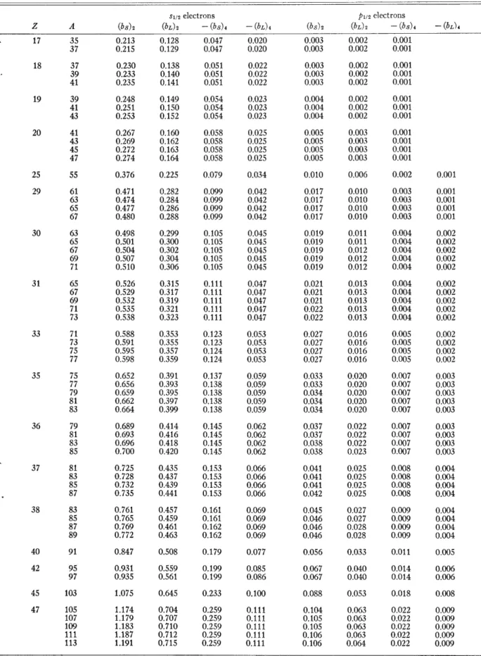
l+a2+a4+a5+a6, a2 = 27rRN3po/3Ze, a₄= rRNp2/5Ze, (n= 1,2). (8) The sum over n results from the series solution of the Dirac equation. The values of the electron coefficients

bs and bL (defined in the Appendix) are given in Table I for s112 and P1/2 electrons as a function of A and Z. Equation (A.12a) gives bD in terms of bs. A plot of these coefficients is shown in Fig. 3. For comparison we also show the results obtained for uniform and surface charge distributions.6 It is interesting to note that the magnitudes of the b coefficients tend to decrease the more the nuclear charge is distributed at larger distances from the center, reflecting the cor-responding changes in the electron binding. Figure 4 compares the b coefficients for the S11₂ and P1/2 states for the charge distribution of Eq. (5).

We have investigated the effect on these coefficients of a modification of the approximate representation of

the charge distribution Eq. (5)] in the form p=pO

+p2X2+p₄X4+p6X6 which in fact gives even a slightly better fit to the trapezoidal distribution than Eq. (5)]. We find that the b coefficients for these two representa-tions agree to within 2.5% for n= 1 and 2. The coefficients for n>2, which are small, are sensitive to such slight variations in p. Since at present there is no experimental evidence in favor of either one, these higher terms cannot be considered to have significance

-n z Z) cr (7) { I-m (7a)

(7a)

a = 2rRN3p3/15Ze, a₆= 27rRNp4/21Ze.

The solution of the Dirac equation for this potential, and the evaluation of the electron integrals of Eq. (4), are given in the Appendix. With these results [Eqs.

19 J. E. Rosenthal and G. Breit, Phys. Rev. 41, 459 (1932).

0 0.2 0.4 0.6 0.8 1.0

r X=

RN

FIG. 2. Charge distribution as given by the representation of Eq. (5). The broken lines indicate the trapezoids used in the determination of the parameters.

/'n --.

~

~ ~ ~ ~ ~ ~

.~~ . ' - I- ._--~~~~~~~~~~~~~~~~~~~~~~~~~~~~~~~~~~~~~~~~~~~~~~~~~~~~~~~~~~~ 1328 flu

(6)

NUCLEAR MAGNETIZATION ON hfs IN ODD-A in the result. As we will show in Sec. V, the evaluation

of the radial nuclear matrix elements involves

(Ro/RN)2", where Ro0= 1.20A t f and is the radial

parame-ter involved in the nuclear potential well. If we take this factor into account, the n> 2 coefficients may affect the value of to about five percent. We note, however, that in the comparison with experiment we take the difference of for two isotopes (see Sec. VI). Therefore if and 2 are very similar, although their differences will be small, the effect of neglecting such higher terms will also be canceled to a large extent. On the other hand if the e are very different, as they would be if the two isotopes have different spins, then the difference will be large, and again the terms n>2 will have relatively little effect. The actual extent of such cancellations will depend on the specific properties of the isotopes under consideration.

IV. EVALUATION OF THE NUCLEAR INTEGRALS 'In Eq. (8) an expression is obtained for the quantity

E which involves calculating the expectation value of

the operators M., where

I-Z C., a: AL (b) ₂ 5 /2 STATE P/2 STATE -(b,)4 (bs)₂ -(b) 4 O50 60 70 80 90 Z

FIG. 4. Dependence on Z of the electron coefficients b for s1/2

and P/2 states for an assumed Hofstadter type of nuclear charge distribution. The b's are defined in the Appendix.

M,= MnSL+MD, and 1 Ri2n MnSL_-- E -[ - s tg) S z() ( bs ) 2n +gL(i)Lz(i) (bL)2n], 1 Ri2 n MnD = - -- gs(i)Dz(i)(bD)2n. t i RN2n

Explicitly for a nucleus of sin j, since the expecta value is to be taken with respect to a nuclear function having its maximum z component of spin require (writing only the angular terms in the follox

(9) three parts)

(12) where (jllMnlj) is the reduced martix element of Mn. (10) C is a Wigner coefficient.

In ignorance of the true nuclear wave function,

(11) some approximate or model wave function has to be

used, and in view of the success of CMT in accounting for magnetic moments, this theory is also used in the following calculations. The basic idea is to write the

vave nuclear wave function T'N as

1, we wing (13) 8 7 6 5 04 a-el_W

UNIFORM CHARGE DISTRIBUTION SURFACE CHARGE DISTRIBUTION HOFSTADTER CHARGE DISTRIBUTION

/

/ / / (b)2 -(b,)4 I -1 -- I- -- - -r' -(b,) ₄ 0 10 20 30 40 50 60 70 80 90 Z

FTG. 3. Dependence on Z of the electron coefficients b for

several nuclear charge distributions. The b's are defined in the Appendix.

where '0o (the zero-order state) represents a simple shell-model configuration and the H'I represent admixed configurations characterized by the variable i. For small mixing coefficients 3(i), the main deviation of the expectation value of M, from that given by the simple shell-model wave function will be that due t6 terms linear in 3(i) and the conditions that such contributions should occur is that tIo and T'I must differ at most by one single-particle state. In addition for MSL the orbital states must be the same (l=0), while for M D states differing by Al=2 may also be

coupled.

We follow the classification and labeling of states suggested by Arima and Horie. Thus the zero-order state configuration is written as jP(J=j), where p is the number of odd particles in the state j and no indication is given of the even numbers of nucleons coupled to zero angular momentum. These latter nucleons, however, play a crucial role in the con-figuration admixtures considered here since these admixed states are those in which a nucleon is excited from or to these states. There are three types of

-

-1329 NUCLEI

*'V =* 0+7 i'00 W(i)\i,

(7)

STROKE, BLIN-STOYLE, AND JACCARINO

TABLE I. Electron coefficients b for a Hofstadter-type charge distribution. Values are in percentages.

Sl2 electrons P1/2 electrons Z A (bs)₂ (bL)2 - (bs)₄ - (bL)4 (bs)₂ (bL)2 - (bs) ₄ - (bL)4 17 35 0.213 0.128 0.047 0.020 0.003 0.002 0.001 37 0.215 0.129 0.047 0.020 18 37 0.230 0.138 0.051 0.022 39 0.233 0.140 0.051 0.022 41 0.235 0.141 0.051 0.022 19 39 0.248 0.149 0.054 0.023 41 0.251 0.150 0.054 0.023 43 0.253 0.152 0.054 0.023 20 41 0.267 0.160 0.058 0.025 43 0.269 0.162 0.058 0.025 45 0.272 0.163 0.058 0.025 47 0.274 0.164 0.058 0.025 25 55 0.376 0.225 0.079 0.034 29 61 0.471 0.282 0.099 0.042 63 0.474 0.284 0.099 0.042 65 0.477 0.286 0.099 0.042 67 0.480 0.288 0.099 0.042 30 63 0.498 65 0.501 67 0.504 69 0.507 71 0.510 31 65 0.526 67 0.529 69 0.532 71 0.535 73 0.538 0.299 0.300 0.302 0.304 0.306 0.315 0.317 0.319 0.321 0.323 0.105 0.105 0.105 0.105 0.105 0.111 0.111 0.111 0.111 0.111 0.045 0.045 0.045 0.045 0.045 0.047 0.047 0.047 0.047 0.047 33 71 0.588 0.353 0.123 0.053 73 0.591 0.355 0.123 0.053 75 0.595 0.357 0.124 0.053 77 0.598 0.359 0.124 0.053 0.003 0.002 0.001 0.003 0.002 0.001 0.003 0.002 0.001 0.003 0.002 0.001 0.004 0.002 0.001 0.004 0.002 0.001 0.004 0.002 0.001 0.005 0.003 0.001 0.005 0.003 0.001 0.005 0.003 0.001 0.005 0.003 0.001 0.010 0.006 0.002 0.001 0.017 0.010 0.003 0.001 0.017 0.010 0.003 0.001 0.017 0.010 0.003 0.001 0.017 0.010 0.003 0.001 0.011 0.011 0.012 0.012 0.012 0.013 0.013 0.013 0.013 0.013 0.004 0.004 0.004 0.004 0.004 0.004 0.004 0.004 0.004 0.004 0.019 0.019 0.019 0.019 0.019 0.021 0.021 0.021 0.022 0.022 0.002 0.002 0.002 0.002 0.002 0.002 0.002 0.002 0.002 0.002 0.027 0.016 0.005 0.002 0.027 0.016 0.005 0.002 0.027 0.016 0.005 0.002 0.027 0.016 0.005 0.002 35 75 0.652 77 0.656 79 0.659 81 0.662 83 0.664 36 79 0.689 0.414 0.145 0.062 81 0.693 0.416 0.145 0.062 83 0.696 0.418 0.145 0.062 85 0.700 0.420 0.145 0.062 37 81 0.725 0.435 0.153 0.066 83 0.728 0.437 0.153 0.066 85 0.732 0.439 0.153 0.066 87 0.735 0.441 0.153 0.066 38 83 0.761 0.457 0.161 0.069 85 0.765 0.459 0.161 0.069 87 0.769 0.461 0.162 0.069 89 0.772 0.463 0.162 0.069 40 91 0.847 0.508 0.179 0.077 42 95 0.931 0.559 0.199 0.085 97 0.935 0.561 0.199 0.086 45 103 1.075 0.645 0.233 0.100 47 105 1.174 107 1.179 109 1.183 111 1.187 113 1.191 0.704 0.707 0.710 0.712 0.715 0.259 0.259 0.259 0.259 0.259 0.111 0.111 0.111 0.111 0.111 0.037 0.022 0.007 0.003 0.037 0.022 0.007 0.003 0.038 0.022 0.007 0.003 0.038 0.023 0.007 0.003 0.041 0.025 0.008 0.004 0.041 0.025 0.008 0.004 0.041 0.025 0.008 0.004 0.042 0.025 0.008 0.004 0.045 0.027 0.009 0.004 0.046 0.027 0.009 0.004 0.046 0.028 0.009 0.004 0.046 0.028 0.009 0.004 0.056 0.033 0.011 0.005 0.067 0.040 0.014 0.006 0.067 0.040 0.014 0.006 0.088 0.053 0.018 0.008 0.104 0.105 0.105 0.106 0.106 0.063 0.063 0.063 0.063 0.064 0.022 0.022 0.022 0.022 0.022 0.009 0.009 0.009 0.009 0.009 0.391 0.393 0.395 0.397 0.399 0.137 0.138 0.138 0.138 0.138 0.059 0.059 0.059 0.059 0.059 0.033 0.033 0.034 0.034 0.034 0.020 0.020 0.020 0.020 0.020 0.007 0.007 0.007 0.007 0.007 0.003 0.003 0.003 0.003 0.003 --- A .... ".,,~ l `-' . _ ^~~I~X1 .YI .--_·_^. -·C·--· -- · -- -1330

(8)

NUCLEAR MAGNETIZATION ON hfs IN ODD-A NUCLEI TABLE I.-Continued. S1/2 electrons P1/2 electrons Z A (bs)₂ (bL)2 - (bs)₄ - (bL)4 (bs)₂ (bL)2 - (bs)4 -(bL)4 48 105 1.224 0.734 0.272 0.117 0.113 0.068 0.024 0.010 107 1.229 109 1.233 111 1.238 113 1.242 115 1.246 117 1.251 49 109 1.286 111 1.290 113 1.295 115 1.299 117 1.304 119 1.308 0.737 0.740 0.743 0.745 0.748 0.750 0.771 0.774 0.777 0.779 0.782 0.785 0.272 0.272 0.273 0.273 0.273 0.273 0.287 0.287 0.287 0.287 0.288 0.288 0.117 0.117 0.117 0.117 0.117 0.117 0.123 0.123 0.123 0.123 0.123 0.123 0.114 0.114 0.114 0.115 0.115 0.116 0.124 0.124 0.124 0.125 0.125 0.126 0.068 0.068 0.069 0.069 0.069 0.070 0.074 0.074 0.075 0.075 0.075 0.076 0.024 0.024 0.024 0.024 0.024 0.024 0.026 0.026 0.026 0.026 0.026 0.027 0.010 0.010 0.010 0.010 0.010 0.010 0.011 0.011 0.011 0.011 0.011 0.011 50 115 1.354 0.812 0.302 0.130 117 1.358 0.815 0.303 0.130 119 1.363 0.818 0.303 0.130 51 119 1.420 0.852 0.319 0.136 121 1.425 0.855 0.319 0.137 123 1.429 0.857 0.319 0.137 125 1.434 0.860 0.319 0.137 52 123 1.489 0.893 0.336 0.144 125 1.494 0.896 0.336 0.144 53 121 1.546 123 1.551 125 1.556 127 1.561 129 1.565 131 1.570 54 123 1.616 125 1.621 127 1.625 129 1.630 131 1.635 133 1.640 135 1.645 55 125 1.688 127 1.693 129 1.698 131 1.703 133 1.708 135 1.713 137 1.717 56 129 1.768 131 1.773 133 1.778 135 1.783 137 1.788 139 1.793 0.928 0.931 0.934 0.936 0.939 0.942 0.969 0.972 0.975 0.978 0.981 0.984 0.987 1.013 1.016 1.019 1.022 1.025 1.028 1.030 1.061 1.064 1.067 1.070 1.073 1.076 0.353 0.353 0.354 0.354 0.354 0.354 0.372 0.372 0.372 0.372 0.373 0.373 0.373 0.391 0.392 0.392 0.392 0.392 0.393 0.393 0.412 0.413 0.413 0.413 0.413 0.414 0.151 0.151 0.152 0.152 0.152 0.152 0.159 0.159 0.160 0.160 0.160 0.160 0.160 0.168 0.168 0.168 0.168 0.168 0.168 0.168 0.177 0.177 0.177 0.177 0.177 0.177 60 143 2.115 1.269 0.507 0.217 65 159 2.626 1.576 0.656 0.281 70 173 3.233 1.940 0.845 0.362 75 186 3.949 2.369 1.084 0.465 0.135 0.081 0.029 0.012 0.136 0.081 0.029 0.012 0.136 0.082 0.029 0.012 0.147 0.088 0.032 0.014 0.148 0.088 0.032 0.014 0.148 0.089 0.032 0.014 0.149 0.089 0.032 0.014 0.160 0.096 0.035 0.015 0.160 0.096 0.035 0.015 0.172 0.172 0.173 0.173 0.174 0.175 0.186 0.186 0.187 0.187 0.188 0.189 0.189 0.200 0.201 0.202 0.202 0.203 0.204 0.204 0.217 0.218 0.218 0.219 0.220 0.220 0.103 0.103 0.104 0.104 0.104 0.105 0.111 0.112 0.112 0.112 0.113 0.113 0.114 0.120 0.121 0.121 0.121 0.122 0.122 0.123 0.130 0.131 0.131 0.131 0.132 0.132 0.038 0.038 0.038 0.038 0.038 0.038 0.041 0.041 0.041 0.041 0.041 0.041 0.041 0.045 0.045 0.045 0.045 0.045 0.045 0.045 0.049 0.049 0.049 0.049 0.049 0.049 0.016 0.016 0.016 0.016 0.016 0.016 0.018 0.018 0.018 0.018 0.018 0.018 0.018 0.019 0.019 0.019 0.019 0.019 0.019 0.019 0.021 0.021 0.021 0.021 0.021 0.021 0.294 0.176 0.068 0.029 0.421 0.253 0.102 0.044 0.589 0.353 0.150 0.064 0.807 0.484 0.217 0.093 79 191 4.587 193 4.594 195 4.601 197 4.608 199 4.614 201 4.621 1331 2.752 2.756 2.760 2.765 2.769 2.773 1.316 1.316 1.317 1.317 1.317 1.318 0.564 0.564 0.564 0.564 0.564 0.565 1.020 1.021 1.023 1.025 1.026 1.028 0.612 0.613 0.614 0.615 0.616 0.617 0.287 0.287 0.287 0.287 0.287 0.287 0.123 0.123 0.123 0.123 0.123 0.123 __ _

(9)

STROKE, BLIN-STOYLE, AND TABLE I.-Continued. S1/2 electrons p/;! electrons Z A (bs)₂ (bL)2 - (bs)₄ - (bL)4 (bs)2 (bL)2 - (bs)₄ - (bL)4 80 193 4.760 2.856 1.380 0.592 1.080 0.648 0.307 0.132 195 4.767 2.860 1.381 0.592 1.081 0.649 0.307 0.132 197 4.774 2.864 1.381 0.592 1.083 0.650 0.397 0.132 199 4.781 2.869 1.381 0.592 1.085 0.651 0.307 0.132 201 4.788 2.873 1.382 0.592 1.086 0.652 0.307 0.132 203 4.795 2.877 1.382 0.592 1.088 0.653 0.307 0.132 81 197 4.945 2.967 1.447 0.620 1.144 0.686 0.328 0.141 199 4.952 2.971 1.448 0.620 1.146 0.687 0.328 0.141 201 4.959 2.976 1.448 0.621 1.147 0.688 0.328 0.141 203 4.966 2.980 1.448 0.621 1.149 0.689 0.329 0.141 205 4.973 2.984 1.449 0.621 1.151 0.690 0.329 0.141 85 214 5.727 3.436 1.741 0.746 1.427 0.856 0.426 0.183 90 228 6.736 4.042 2.159 0.925 1.826 1.096 0.576 0.247 95 242 7.716 4.630 2.609 1.118 2.254 1.352 0.751 0.322 100 256 8.476 5.086 3.025 1.296 2.643 1.586 0.931 0.399 to be considered-referred to Type I Excitation

The zero-order configuration has p (odd) particles in state j, nl (even) in jl and n2 (even) in j2, the nl and

n2 particles being coupled separately to zero angular momentum so that the total angular momentum J of the state is equal to j. Thus, symbolically, the state can be written

'Po=I(joln(O)j"

2(0)jP(j)J =j). (14)

The admixed states of type I are then taken to be those in which a particle is excited from state j to state j2, each group coupling respectively to jl and j2, and the jl and j2 coupling together to J1 which couples finally with j to give J =j. The nuclear state TN can therefore be written, on including one such admixture,

*IN='I'(jln'(0)j22(O)jP(j)J =j)+- Jol f(J1)

XTI([jL1?-O (jl)j2fn+ (j)] (Jl)j(j)J=j). (15) Of course, the states jl and j2 are chosen so that the first-order matrix element of Mn is nonvanishing and so that the excitation involved is compatible with the exclusion principle.

Using the results of Noya et al. specialized to our case, the following expression is obtained for the contribution of such a type I mixing to the reduced matrix element of Mn evaluated with respect to (15): (jP J=jMn|[jP J=j)I =-(2j+ 1)C(jlj; ½0) X [nl (2j2+ 1-n2)/(2jl 1) (2jo+ 1)] XhIZli(loj,l2j2) 2) --V I(jlj2j2)/AE, (16) where20 hlti(lojl,l2j2) and = (2j 1+ 1)C(julj2; 5o)(jhllMnllj2)(1-6o), 1 X I (jljj2) = - Rj (R)Rj₂(R)Rj2(R)R 2dR. 2 Jo (17) (18) The upper (lower) line in the bracket ( } must be used when the excited nucleon in the orbit jl is different from (similar to) the nucleon in the orbit j. The quantity -(--1)it-i(j+ ) is to be taken with the --+ sign for excitations with AlI=0, and - sign for Al= 2 in Eq. (17).

In the above expressions, the admixture parameters

fl(J1) have been calculated by straightforward first-order perturbation theory using as the perturbing potential a delta-function interaction given by

V12 V (1 -1 * a2)/4

+ Vt(3+a,- r)/48(R1-R2), (19)

where V, and Vt represent the singlet and triplet strengths of the internucleon interaction. E is the energy needed to excite a particle from the state j to the state j2, and (j1llM.llj2) is the single-particle

reduced matrix element of the operator Mn. Now for

M"SL the only nonvanishing reduced matrix element

to be considered here21 is that for which the particle excitation is from jo=l + to j2=l 1-. However, for

M.D we can have both jl=l+ to j2=l-- and also

20 According to our calculations, Eq. (3.7) of Noya et al. is in error by a factor (2j2+1)'. With our choice of phase in the reduced matrix elements, we also differ in sign in this equation. Our 0 is equal to their e.

21 There is also the possibility of an excitation to a state of the

samej and value but different n value. Such an excitation would be through essentially two oscillator shells and because of the associated large value of AE such excitations are neglected.

excitation which need as types I, II, and III.

--- "~~~~~~~~~~~~~~~~~~~~~~~~~~~~~~~~~~~~~. .~~~~~·1·· 1-·1-~ . . -

-··

_-____

_____I^

_

(10)

NUCLEAR MAGNETIZATION ON hfs IN ODD-A NUCLEI

j=l= I+ 1 to j₂= --1 2 or vice versa. The reduced matrix elements of Mn in each of these cases can be con-structed easily from the single-particle reduced matrix elements of Sz, Lz, and Dz given in Table II.

Using the foregoing relationships, we obtain finally for the contribution of type I admixtures to the matrix elements Mn the expressions given in Tables III and IV, where the radial matrix elements g,(n2,j2,l 2; n1,j1,l1)

are given by g,(n2,j2,12; nl,jl,ll) R2n =

J

Rn 2 2z2(R) -l Rt l31(R)R2dR. (20)

0

RN2 n

Here the radial functions are those describing the ground and excited states of the single particle involved in the type I excitation; the evaluation of the ,n and also the estimation of the AE will be discussed in Sec. V.

Type II Excitation

In this type of excitation, the orbit j2 (of type I

excitation) coincides with j. Thus the nuclear wave function, including a typical type II admixture, can now be written

,N= I(jl (0)j (j)J=j)

+YJ,1 (Jl)TI(jln-l(jl)jP+l(Jl)J =j), (21)

where p and n are the numbers of odd and even nucleons, respectively. Using the same interaction as in type I and specializing the results of Noya et al. to

TABLE II. Reduced matrix elements (jlllMllj 2) of

operators S, L, and D. Operator M l1-12 jl-j2 (jlMlIi2) S 0 1 -[(2j+1)(2j2+l)/j] L 0 1 ½[(2j+1) (2j2+1)/ij0] D 0 1 -8[L(2ij+l)(2j2+ 1)/j,]i S 0 -1 2[(2j1+1)(2j2+l)/j2] L 0 -1 -2 (2j1+ 1) (2j2+l)/j2] D 0 -1 [ (2j+ 1) (2j2+)/j2]i D 2 1 0Lli(li-1)/2(21-l)]* D -2 -1 -2[1 2(l2-1)/2(212-1)]

our case, we have (jPJ=jll MnI jpJ =j)II

=-(2j+1)iC(jlj; 0)[n/(2j+ 1)]

X (2j-p)/(2j- 1)]hli'i(lji,lj)

X (- V,)I(jj3)/AE, (22)

where the various components of this expression are defined as in Eqs. (17)-(19). The contributions of this type II admixture to the matrix elements Mn are given in Tables V and VI where the radial matrix elements g are defined as in Eq. (20).

Type III Excitation

Here the orbit jl coincides with the orbit j (of type I excitation). The nuclear wave function including an admixture of this type can now be written

TIN= Tk(jl (O) jP (j)J=j)

+EJ I(Ji)TxI' +(jl(j)jv- (J')J=j), (23) TABLE III. Contributions of type I admixtures to M,; the excitation is one of an even number nl particles in orbit j =l,+2 to orbit

j2=lt- containing an even number n2 particles. Note that for (bs)2n= (bL)2n= gn=/= 1, (bD)2n=O, the values of M, given by this

table are just those obtained by Arima and Horie3for 3,UI.

Contribution from

Nucleus j Mu/[n1l(2j2+l-n2)/(2j2+1)] even numbers of

- (l+2)ll₁[gs((bs)2 - (bD)2)-gL(bL)21],(n1, 11+2, 1l; n2, 1l- 1) V I/AE protons (neutrons)

l+½

(21+3) (21+1) [1 (Vt- V8)I/AE neutrons (protons)

Odd proton

(neutron) (I- 1)l[gs((bs)2-(bD)2n)-gL(bL)2n].&(nl, I+, ,; n2, 11-11) E protons (neutrons)

I- -2 -/-V AE pr

(21+1) (211+1) 2 (Vt-Vs)I/AE neutrons (protons)

TABLE IV. Contributions to MD for admixtures of type I with Al= 2. If jl <j2, 12 is larger; for jl >j2, 1l is larger.

We denote the larger I by 1>.

Contribution from

Nucleus j -M,D/[n 1(2j2+l -n2)] even numbers of

- (3/8)lgs(bD)29(nl,jl,ll; n2,j2,12) - VI/AE protons (neutrons)

(21+3) (21>- 1) ½ (Vt- V.)I/AE neutrons (protons) Odd proton

(neutron) (3/8) (1+l )gs (bD)2nn (nl ,jl,li; n2,j2,12) - VII/AE protons (neutrons)

(21+1) (21>- 1) I (Vt- V.)I/AE neutrons (protons) 1333

(11)

TABLE V. Contributions of type II and III admixtures to Mn. Type II is the excitation of an even number n particles in orbit ji=l+, into the odd group j = l- containing p particles. Type III is the excitation of the p particles in the odd group j = l+ into the orbit

jl=l- containing n particles. If we specialize as in Table III, M. are again the results of Arima-Horie3 for 8

#In and 6pIII. For the latter, usually n =0.

Excitation type MnEu

n(2j-p) (l- )lEgs((bs) 2n-4 (bD) 2)-gL(bL) 2,] (n, j =1+2, 1; n,j=l--, l) (- V,₈1/E)

(2j- 1) (21+1)2

- (P- 1) (2j1+ -n) (1+1) (I +2)[gs((bs)2- (bD)2--gL(bL) ],I(nj=l+1, 1; n, jlI=---, 1) (-- VI/AE)

III 3

(2jl+1) (21+1) (21+3)

and the appropriate reduced matrix element is (jPJ=jlMll jPJ=j)III

-(2j+ 1)IC(jlj; 0)[(2jl+ 1-n)

X (p- 1)/ (2j+ 1) (2j- 1)]h~i(l- j1,lj)

X (- V)I(jlj3)/aE. (24) The contributions to M, resulting from this type of admixture are listed in Tables V and VII.

and for j= l- 2,

/1f

§ 2j+3 1

M.= g-) j gL (bL) 2 - (gs)

Pt\b)n 2j+2 2j+2

X[(bs)2. (2j3) njl ), (26) where in both expressions all the symbols have been defined previously.2 4

Zero-Order Term

Finally an expression has to be given for the reduced matrix element of M, with respect to the zero-order function P(jP(j)J=j). Only the odd (p) particles will contribute to this matrix element and we obtain in a straightforward fashion

Mn= C(jlj; jO)(jPJ =jllMnlljP =J) =C(jlj;jO)(jllMnllj)

for p identical particles.22'23 Thus for j= 1+-,

(25)

TABLE VI. Contributions to MD for admixtures of type II with Al= 2.

j -,uMD/[n(2j-p)] - (3/8) (l+1)gs(bD)2fl4n,(n, jl,ll; n,j,l) (- VI/AE) 1+3 j,>j (21+3)2 (3/8)l( 1)gs (bD)2 9, (n.l jl,ll; n,j,l) (- V.I/AE) I-- jl <j (I-1) (412-1)

22 G. Racah, Phys. Rev. 63, 367 (1943).

23 C. Schwartz and A. de-Shalit, Phys. Rev. 94, 1257 (1954).

V. RADIAL MATRIX ELEMENTS AND NUCLEAR

ENERGY LEVELS

Evaluation of ,J(n,j2 2,12; ni,jl,l,) and AE

In order to obtain values for the radial integrals n for two single particle states n2j212 and njl1l, the

following approach was adopted. The relevant single-particle wave functions and energies were calculated for particle motion in a nuclear potential well of the Saxon-Woods type having the form

I IV

1

V(R)=

1+exp[Ao(R-Ro)]

tKA2 Ao0 VolexpEAo(R-Ro)]

4m2c2{ l+exp[Ao(R-Ro)]}2R (27)

Coulomb effects were taken into account by assuming that the protons also moved in the potential of a charge distribution p(R) of the form

po[1+R2/RC2]

(28) so normalized that the resulting Coulomb potential

V,(R) satisfied

V,(R) -- (Z-l1)e2/R for R-- oo.

2 The subscript n is used variously denoting in the nuclear radial integrals the principal quantum number, in the angular matrix elements, numbers of particles, and thirdly the terms arising from the series expansion of the Dirac equation. The particular meaning is obvious from the context.

~_

l~C---·~---^--·I. -LI_ -·l-P~lll_ -. . ..( ll·-L~·· ·

~^_-·I

.-- II · I~ I

1334 _TN-"' " ,,,I/ 1+ expCE 1(R- R,)] M."=-l gL(bL)2(j-2) 2j- 1

~

(12)

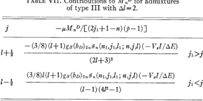
NUCLEAR MAGNETIZATION ON hfs IN ODD-A NUCLEI TABLE VII. Contributions to MD for admixtures

of type III with Al= 2.

j -uMnD/[(2ji+ 1-n) (p--1)]

- (3/8) (l+1)gs(bD)2,,(n,j,1; n,j,l) (- V,I/AE)

(21+3)2

1-- jz <j

(l-1) (412 - 1)

The well radii Ro and R, are defined by Ro = roA ,

R,=CRo, and the various values of the parameters

used are as follows:

Vo = 64.5 Mev for an odd proton, K = 3 9.5,

V0= 50.0 Mev for an odd neutron, C= 0.96, ro= 1.20X 10-13cm,

A0 = 1.40X 10-13 cm-',

TABLE VIII. Values in Mev of energy differences AE required

for calculations of e. These are obtained from the work of Arima and Horie (see references 3 and 25).

States AE States AE States AE

ld5/2-d3/2 5 lgg/2-lg7/2 2.5 lhg/2-2f7/2 0.5 2s1/2--1d3/2 4 lg7/2-2d5/2 0.5 2 f7/2-2f5/2 1.5 lf7/2-lf5/2 3 2dS/2-2d3/2 1.5 2f5/2-3p3/2 0.75 2p3/2-2pl/2 1.5 2d3/2-3s1/2 0.25 3 P3/2-3Pui2 0.5 2 P3/2- f5/2 0.5 lh/112- 22 lil/-i9/2

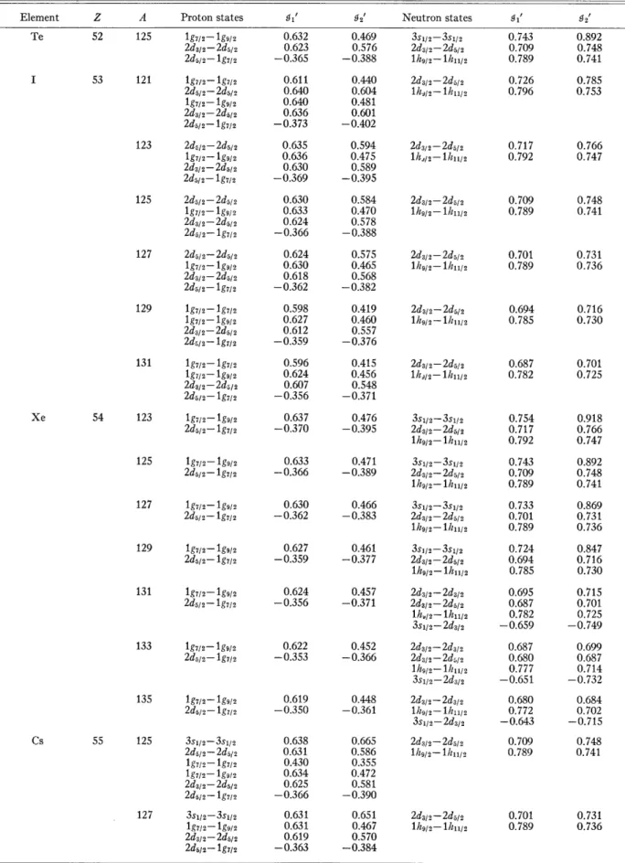
In Table IX the final results for ,/(nl,ll,j; n2,12,j2)

are given, but it must be remembered that in using this table the relation of Eq. (31) must be used in order to obtain g,(n,l,jl; n2,12,j2). The program also

printed out the radial wave functions, binding energies,

g93, and 4t .

A 1 = 1.40X 10-13 cm-1.

These values lead to an approximately correct ordering of the single particle neutron and proton energy levels. We adopt the values of E as given by Horie and

Arima25 who discuss their determination in detail.

Our parameters are thus consistent with the ones used in their magnetic moment and electric quadrupole calculations. The pertinent energy denominators are reproduced in Table VIII.

The calculations of the wave functions, energies, and finally the radial matrix elements were carried out on the Mercury computer at Oxford using a program due to Dr. L. M. Delves.

The radial integrals required are of the form

g

=R

N2 R,(R)R2+2R2(R)dR, (29)

where RN is the full radial extent of the trapezoidal charge distribution and is defined in Sec. III. In the machine calculations, the actual radial integrals calculated were

Rn 2

f

R(R)R2'+2R2(R)dR, (30)

where Ro is involved in expression (27) for the nuclear potential distribution. Thus a. and g.' are related by

Ro2 \ n 1.20A 2n

g,=(-} ..= . / a (31)

RN2 j 1.07A t+ 1.50/

where we have used the expression RN given in Sec. III.

26 H. Horie and A. Arima, Phys. Rev. 99, 778 (1955).

Values of V, Vt, and I

In estimating the values of these three parameters, we follow the procedure of Arima and Horie and take

IVtl 1.51 V

1.

We further ignore the dependence of the integrals I [Eq. (18)] on the quantum numbers involved and only take into account the approximate mass dependence of I. The value of the product VI is related to pairing energy data and, following Arima

and Horie, we take VI= -25/A Mev.

VI. COMPARISON WITH EXPERIMENTAL RESULTS AND DISCUSSION

General Expression for e

We now consider the general form taken by e when many admixtures of different types are contributing. By Eq. (8),

-e=E N*MNdrN= E M,

n= ,2 n=1,2

(32)

where M, is the operator defined in (9), and where.

IkN may contain the three types of admixtures described.

It must be remembered in this connection that there may be several different admixtures of each type contributing. Now it is of interest and of some practical use to write down in a semi-symbolic way the form taken by -E taking into account all of the possible

first-order admixtures investigated. Referring to

Tables III through VII, and Eqs. (25) and (26), it

26 H. H. Stroke and R. J. Blin-Stoyle, Proceedings of the International Conference on Nuclear Structure, Kingston, edited by D. A. Bromley and E. W. Vogt (University of Toronto Press, Toronto, 1960), p. 518.

--

(13)

TABLE IX. Values of radial integrals 6,' between single-particle states nlljl and n22j2 required for the calculation of hfs anomalies. For states which are unbound with the parameters indicated in the text, the program increases the well depth to give a binding energy E= 0.

Element Z A Proton states ls' 42' Neutron states s' a2'

Cl 17 35 ld3/2- d3/2 0.686 0.641 ld312- d5/2 0.800 0.876 Id3/2- ld5/2 ld3/₂-21/2 37 Id3/2-- ld32 ld312-- ld52 ld/2-2sl/2 Ar 18 37 ld3/2- ld5/2 ld3/₂- 2s1/2 39 ld3/2-- d5/2 ld3/₂- 2s/2 41 ld3/2-- 1d5/2 ld3/2- 2S1/2 K 19 39 ld3/2-1d3/2 41 ld3/2- 1d3/2 43 Id3/2- 1d3/2 Ca 20 41 43 45 47 Cu 29 61 2P3/2-2p3/2 lf5/2- 1f7/2 63 2P3/2-2 p3/2 lf5/2- lf7/2 65 2P3/2-2p3/2 lf5/2- lf7/2 67 2p3/2-2p3/2 lf5/2- lf7/2 Zn 30 63 2p1/2-2P3/2 lf5/2- 1f7/2 2 P3/2- lf5/2 65 2pl/2-2p3/2 lfl/2- 1f7/2 2 p3/2- 1f5/2 67 2p/2-2p3/L lfs/2- lf7/2 2 p3/2- lf5/2 69 2pl/2-2p3/2 lfs/2- lf7/2 2p3/2- 1f5/2 71 2P1/2-2p3/2 lf5i2- 1f7/2 2 p3/2- lf5/2 0.689 -0.616 0.662 0.669 -0.590 0.670 -0.592 0.653 -0.570 0.638 -0.551 0.644 0.626 0.610 0.721 0.690 0.706 0.680 0.692 0.670 0.679 0.661 0.716 0.680 -0.513 0.700 0.671 -0.500 0.685 0.662 -0.489 0.672 0.654 -0.479 0.659 0.646 -0.469 0.629 -0.700 0.592 0.590 -0.646 0.592 -0.648 0.559 -0.603 0.531 -0.565 0.555 0.521 0.492 ld3/2- 1d3/2 f7/2- If7/2 lf7/2- lf7/2 lf5/2- 1f7/2 l15/2- f7/2 lf5/2- lf7/2 lf7/2- lf7/2 lf7/2- lf7/2 lf5/2- lfI/2 f7/ 2- f712 lf5/2- 1f7/2 If/ 2- 1f7/2 lf5/2- 1f7/2 0.804 2pl/2-2P./2 0.590 lf/2- lf7/2 2p3/2- lf1/2 0.770 2pl/2-2p3/2 0.571 lfs2-- lf7/2 2p3/2- lf5/2 0.740 2p1/2-2p3/2 0.554 lf5/2- 1f7/2 2p3/2- lf5/2 0.713 0.538 2 Pl/2-2p3/2 0.794 lf5/2- lf5/2 0.572 2p3/2-2p3/2 -0.582 2pl/2-2P3/2 fs5/2- 1f7/2 2 p/2- lf1/2 0.758 fs5/2- lf5/2 0.555 2P3/2-2p3/2 -0.557 2P1/2-2P3/2 lf5/2- 1f7/2 2 p3/2- 1f5/2 0.727 0.539 -0.534 0.699 0.525 -0.514 0.673 0.512 -0.497 lf5/2- 1f5/2 2 pl/2-2P3/2 2 pl/2-2pl/2 2 P1/2-2pl/2 lg9/₂- lg/2 0.788 0.994 0.962 0.993 0.993 0.974 0.962 0.935 0.974 0.910 0.952 0.889 0.932 0.892 0.781 -0.654 0.865 0.767 -0.631 0.840 0.754 -0.612 0.818 0.770 0.839 0.865 0.767 -0.631 0.753 0.818 0.840 0.754 -0.612 0.737 0.818 0.819 0.798 0.893 0.874 1.292 1.199 1.40 1.40 1.32 1.199 1.122 1.32 1.056 1.26 1.000 1.20 1.250 0.777 -0.902 1.173 0.745 -0.846 1.106 0.717 -0.798 1.047 0.781 1.098 1.173 0.745 -0.846 0.739 1.043 1.106 0.717 -0.798 0.703 1.047 1.048 0.993 0.965 1336 .- 1----1· ·111_11·· _. . . .

(14)

NUCLEAR MAGNETIZATION ON hfs

TABLE IX.-Continued.

Element Z A Proton states al' 92' Neutron states gl' 2'

Ga 31 65 2p312-2p3/2 0.694 0.745 2P1/2-2p3/2 0.840 1.106 2pl/2-2p3/2 0.701 0.761 lf5/2- lf7/2 0.754 0.717 lf5/2-- lf7/2 0.671 0.556 2P3/2- lf5/2 -0.612 -0.798 2p312- f51 2 -0.501 -0.558 67 2p312- 2p3/2 0.681 0.717 2P1/2-2p3/2 0.818 1.047 2 P1/2-2p312 0.686 0.730 1f512- lf712 0.742 0.691 lf/2- f7/2 0.663 0.541 2P3/2-lf5/2 -0.594 -0.756 2P3/2- lf5/2 -0.490 -0.536 69 2P3/2-2p3/2 0.669 0.692 2pl/2-2Pa3/2 0.798 0.994 2 p1/2-2p3/2 0.673 0.701 if 5/2-lf 712 0.654 0.526 2p31/2- lf512 -0.479 -0.516 71 2p3/2-2p3/2 0.658 0.669 2pll/2-2p3/2 0.780 0.948 2pl/2-2p3/2 0.660 0.675 lg712- lg9 2 0.873 0.972 lf5/2-- lf7/2 0.647 0.513 2p3/2- lf/₁2 -0.470 -0.498 73 2p3/2-2p3/2 0.647 0.648 2pl/2-2p3/2 0.763 0.907 2pl/2-2p3/2 0.649 0.651 1g7/2-lg9/2 0.898 1.04 lfl52- lf7/2 0.640 0.501 2p3/2- lf5/2 -0.461 -0.482 As 33 71 2p3/2-2p3/2 0.660 0.673 2pI/2-2p3/2 0.780 0.948 2P1/2-2p3/2 0.662 0.680 lf5/2- lf7/2 0.648 0.515 2p3/2- lf5/2 -0.471 -0.501 73 2p3/2-2p3/2 0.649 0.652 2pl/2-2p3/2 0.763 0.907 2pl/2-2p3/2 0.651 0.656 lg712-lgg/2 0.898 1.04 lf52- f7/2 0.641 0.503 2 p3/2- If/2 -0.462 -0.484 75 2p3/2-2p3/2 0.639 0.632 2pl/2-2p3/2 0.747 0.869 2p1/2-2p2/ 0.640 0.634 lg712-lg/2 0.891 1.02 lf6/2- lf7/2 0.634 0.491 2p/312-lf/2 -0.454 -0.469 77 2pa- 2 312 0.630 0.614 2pl/2-2p3/2 0.732 0.834 2pl/2-2p3/2 0.630 0.614 lg7/2-lg/2 0.882 0.990 f1/2- lf7/2 0.628 0.481 2p3₁₂-lf5/2 -0.446 -0.455 Br 35 75 2p3/2-2p312 0.640 0.635 2pl/2-2p3/2 0.747 0.869 2pl/2-2p3/2 0.641 0.638 lfl2- f7/2 0.635 0.493 2p3/2- f5/2 -0.454 -0.471 1g7/2- lg/2 0.742 0.671 77 2p3/- 2p312 0.632 0.617 2pl/2-2p.3/2 0.732 0.834 2 pr/2-2pd/2 0.631 0.618 lg7/2- lg9/2 0.882 0.990 1f5/2- lf7/2 0.629 0.483 2p3/2- lf12 -0.447 -0.458 lg7/2-lg/2 0.738 0.662 79 2p3/2-2p3/2 0.623 0.600 2pl/2-2p3/2 0.724 0.814 2 pl/2 2p3/2 0.622 0.599 lg7/2- lg9/2 0.847 0.902 lf5/2- f7/2 0.623 0.473 2 p3/2- lf512 -0.440 -0.445 lg7/2- lg9/2 0.735 0.654 81 2p3/2-2p3/2 0.615 0.584 2pl/2-2P3/2 0.707 0.777 2p1/2-2P3/2 0.613 0.582 lg7/2- 1g/2 0.840 0.886 f5/2- 1f7/2 0.617 0.464 2 p3/2- lf5l/2 -0.434 -0.433 1g7/2-lg g/2 0.731 0.646 83 2p3/2-2pS/2 0.607 0.570 2pl/2-2p3/2 0.699 0.759 2pl/2-2p3/2 0.604 0.566 lg7/2-lg9/2 0.834 0.870 lf5/2- lf7/2 0.612 0.455 2p3/2- lf~b/2 -0.428 -0.422 1g₇/₂-lg/2 0.728 0.638 1337 IN ODD-A NUCLEI

(15)

Element Z A Proton states al' 92' Neutron states gl' a2'

Kr 36 79 2pl/2-2p3/2 0.622 0.601 2P1/2--2p12 0.734 0.836

-- - - ,

---(---_I--~~~~~~~~~~~~~~~~~~~~~_·---·-· Il L~~~~~~~~~~~~~~~~~~-..~~~

~. ~~·~-1~·_·__-l-m-LI

STROKE, BLIN-STOYLE, AND JACCARINO 1338

lf52- f7/2 2p3/2- lf5/2 81 2p/2-2p3/2 l /2- lf7/2 2p3/2- lf6/2 83 2p1/2-2p3/2 lf6/2- lf7/2 2p3/2- lf5/2 85 2pl/2-2p3l2 lfb/ 2-1f7/2 2p3/2- 1f56/2 Rb 37 81 2p3/2-2p3/2 2pl/2-2p3/2 83 lf6/2- f5/2 2pl/2-2p3/2 85 lf/2-lf5/2 2pl/2-2p3/2 87 2p3l/2-2p3/2 2pl/2-2p3/2 Sr 38 83 2pl/2-2p3/2 0.624 -0.441 0.614 0.618 -0.434 0.605 0.613 -0.428 0.597 0.608 -0.422 0.616 0.614 0.588 0.606 0.583 0.598 0.594 0.590 0.606 0.474 -0.446 0.583 0.465 -0.434 0.568 0.456 -0.423 0.553 0.448 -0.413 lg7/2- g9/2 2pl/2-2p3/2 lg19/2- 1g9/12 l7/2-- g9/2 2pl/2-2p3/2 lg9/2-- lg9/2 lg7/2- 1g9/2 2pl/2-2p3/2 lgg/92- 1g9/2 lg72- lgg9/2 0.847 0.724 0.842 0.840 0.707 0.830 0.834 0.699 0.821 0.822 0.902 0.814 0.847 0.886 0.777 0.819 0.870 0.759 0.800 0.840 0.587 lg7/2- lg9/2 0.585 2pl2-2p3/2 0.423 lg7/2- g9/2 0.569 2pl/2-2p3/2 0.414 lg7/2- lg9/2 0.554 2pl/2-2p3/2 0.840 0.707 0.834 0.699 0.822 0.684 0.810 0.830 0.834 0.699 0.821 0.822 0.684 0.813 0.810 0.909 0.799 0.865 0.907 0.774 -0.567 0.850 0.887 0.766 -0.546 0.734 0.815 -0.501 0.727 0.801 -0.491 0.722 0.788 -0.483 0.776 0.765 0.805 0.791 0.815 0.734 -0.501 0.886 0.777 0.870 0.759 0.840 0.726 0.811 0.819 0.870 0.759 0.800 0.840 0.726 0.783 0.811 1.241 0.786 1.11 1.24 0.729 -0.786 1.07 1.19 0.711 -0.742 0.646 0.996 -0.640 0.633 0.962 -0.620 0.622 0.930 -0.602 0.901 0.874 0.780 0.930 0.996 0.646 -0.640 0.546 0.540 lg7/2- g9/2 0.570 lg9/2- lg912 lg?7/2- lg/2 2pl/2-23/2 0.556 lg9/2- lg9/2 lg?2-- lg92 2pl/2-2p3/2 0.542 lg/2- lgg/2 lg7/2- lg/2 0.529 2d/2-2d5/2 lg7/2- lg9/2 0.499 2d5/2-2d5/2 0.573 2d3/2-2d5/2 lg7/2- lg9/2 2d/2- lg7/2 0.489 2d5/2-2d5/2 0.562 2d3/2-2d412 lg7/2-- lg/2 2d612- lgi/2 0.451 lg7/2- lg/2 0.530 2d3/2-2d5/2 2d5/2- 1g7/2 0.443 lg7/2- lg1/2 0.522 2d3/2-2d5/2 2d/2-- lg7/2 0.435 lg7/2- lg,/2 0.514 2d3/2-2d5/2 2d5/2- lg7/2 85 2pI/2-2p3/2 87 2PI/2-2P3/2 89 2pl/2-2p3/2 Mo 42 95 2pl/2-2p3/2 lg1/2-- lg9/2 97 2P/2-2P3/2 lg7/2- lg/2 Ag 47 105 2pl12-2p1/2 lg7/2- lgy/2 107 2pl/2-2pl/2 lg72- lg/2 109 2pl/2-2p/2 lg7/2- lg9/2 111 2p1/2-2p1/2 lg7/2- lg9/2 113 2pl/2-2pl/2 lg7/2- lg9/2 Cd 48 105 lg7/2- lg9/2 2pl/2-2p3/2 0.598 0.591 0.584 0.567 0.694 0.561 0.688 0.540 0.669 0.535 0.664 0.530 0.660 0.526 0.656 0.521 0.652 0.670 0.546 0.428 0.507 2d3/2-2di/2 0.421 2d3/2- 2d5/2 0.500 lh,/2-- kl/2 0.531 2d5/2-2d5/2 0.464 2d3/2-2d5/2 lg17/2-- lg/2 2d5/2-- g7/2

(16)

NUCLEAR MAGNETIZATION ON hfs IN ODD-A

TABLE IX.-Continued.

Element Z A Proton states 41' 42' Neutron states 1/ 42'

Cd 48 107 ₂1g7/2-- lg9/2 0.665 0.523 2d5/2-2d5/2 0.780 0.904 pl/2- 2P3/2 109 1g7/2- 1g9/2 2 pl/2-2p3/2 111 1g7/2-- 1g9/2 2P1/2-2P3/2 113 lg?12-lg91/2 2 P1/2-2P3/2 115 1g712-- 1g912 2p1/2-23/12 117 1g7/2-1g912 2 P1/2- 2P3/2 In 49 109 1g₉12- 1g91/2 1g712- lg9/2 111 lgg/2-- g9/2 1g7/2- lg9/2 113 1g9/2-- 1g912 1g7/2- 1g₉/2 115 1g9/2- 1g₉/2 1g7/2-- 1g9/2 117 1g9/2-1 g9/2 1g7/2- lg9/2 119 lgg/2--lg12 lg,/2- 1g9/2 Sn 50 115 1g7/2- 1g9/2 117 1g7/2- 1g9/2 119 1g7/2- 1g9/2 Sb 51 119 2d5/2-2d 1/2 1g7/2- 1g712 g?7/2- lg9/2 121 2ds/2-2d/21 1g?7/2-- lg9/2 123 1g7/2-1 g7/2 1g7/2- 1g₉/2 125 1g7/2-1 g12 2d5/2-2d/2 1g7/2- 1g₉/2 Te 52 123 1g712-1g₉12 2d3/2-2d5/2 2d5/₁₂- 1g7/2 0.541 0.660 0.537 0.656 0.532 0.652 0.528 0.648 0.524 0.644 0.520 0.700 0.661 0.696 0.657 0.693 0.652 0.689 0.648 0.686 0.645 0.683 0.641 0.649 0.645 0.642 0.645 0.614 0.642 0.639 0.639 0.607 0.635 0.604 0.628 0.632 0.636 0.629 -0.369 0.456 2d3/2-2d5/2 1g7/2-- 1g9/12 2d5/₂-1g7/2 0.515 2d5/2-2d 5/2 0.449 2d3/2-2d5/2 1g7/2- 1g9/2 2d₅/2- g7/2 0.508 3s1₁/2-3s11/2 0.442 2d3/2-2d51 2 1g7/2- 1g₉/2 2d₅/₂-- 1g7/2 0.501 3S1/2-3s11/2 0.435 2d3/2-2d5/2 0.495 3s1/2-3s/2 0.428 2d3/₂-2d5/2 lh912- lh111 2 0.488 3S1/2-3s1/2 0.422 2d3/2-2d5/2 lh₉₁₂-lhk1₁₂ 0.565 1g7/2- lg9/2 0.516 2d3/2-2d5/2 2d5/₂- lg7/2 0.559 1g7/2- 1g₉/2 0.509 2d3/2-2d5/2 2d5/₂-1g7/2 0.553 1g7/2- 1g₉/2 0.502 2d3/2-2d512 0.547 2d3/2-2d5 12 0.495 lh9/2- lhl11 2 0.541 2d/2-2d5/2 0.489 lh9 12-lhk 11 2 0.536 2d3122d-- 12 0.483 lh9a2-- Ihll2 0.496 3s1/₂-3s1/2 2d3/2-2d/2 0.490 3s112-3s1/2 2d3/₂- 2d5/2 lh91 2- Ihk112 0.484 3S12-3s11/2 2d3/2-2d5/2 lhg9/2-- lh11/2 0.612 0.444 0.485 2d312 - 2d/12 lh912-lhn12 0.601 2d3/2- 2d5/2 0.479 lh/9 2-lh 1112 0.433 2d3/2 - 2d1/2 0.474 lk9/2- h11/2 0.428 0.581 0.469 2d3/2- 2d1/2 lh9/2-- l112 0.474 3s1/2-3s1/2 0.587 2d3/2--2ds/2 -0.394 lh/12- l111t2 0.801 0.727 -0.491 0.770 0.788 0.722 -0.483 0.832 0.776 0.716 -0.475 0.817 0.765 0.803 0.754 0.802 0.789 0.744 0.801 0.722 0.788 -0.483 0.716 0.776 -0.475 0.710 0.765 0.754 0.802 0.744 0.801 0.735 0.797 0.803 0.754 0.789 0.744 0.801 0.777 0.735 0.797 0.735 0.797 0.726 0.796 0.717 0.792 0.709 0.789 0.754 0.717 0.792 0.962 0.633 -0.620 0.880 0.930 0.622 -0.602 1.113 0.901 0.611 -0.585 1.074 0.874 1.038 0.849 0.773 1.004 0.826 0.766 0.622 0.930 -0.602 0.611 0.901 -0.585 0.601 0.874 0.849 0.773 0.826 0.766 0.805 0.760 1.038 0.849 1.004 0.826 0.766 0.973 0.805 0.760 0.805 0.760 0.785 0.753 0.766 0.747 0.748 0.741 0.918 0.766 0.747 NUCLEI -- -- -1339

(17)

Element Z A Proton states al' 92' Neutron states gl' 92'

Te 52 125 le7/2- la/2 0.632 0.469 3s,1--3sv2 0.743 0.892

~~~~~-

1 1~~~~~~~~~~~~~~~~~~~1---1~~~~~~~~~~~~~~~~~~~~~~~.. ._

S ., ..-- · ·

~

- --

STROKE, BLIN-STOYLE, AND JACCARINO 1340

2d3/-2d5/2 2d5/2- 1g7/2 53 121 lg7/2- lg/2 2d5/2-2d512 lg7/2- lg9/2 2d/2-2ds/2 2d5/2- lg7/2 123 2d5/2-2d5/2 lg7/2- lgg/2 2d3/2-2d5/2 2ds/2- lg7/2 125 2ds/2-2d/2 lg7/2- lg9/2 2d3/--2d5/2 2d/2-- lg7/2 127 2ds/2-2d5/2 lg7/2-- lg91/2 2da/2-2d/2 2d/2-- lg17/2 129 lg7/2-- lg7/2 lg7/2- lg9/2 2d/2- 2ds/2 2dr/2-- lg2/ 131 lg7/2- 1g7/2 lg7/2- lg/2 2d3/2-2d512 2ds5/2-- lg7/2 0.623 -0.365 0.611 0.640 0.640 0.636 -0.373 0.635 0.636 0.630 -0.369 0.630 0.633 0.624 -0.366 0.624 0.630 0.618 -0.362 0.598 0.627 0.612 -0.359 0.596 0.624 0.607 -0.356 0.637 -0.370 0.633 -0.366 0.630 -0.362 0.627 -0.359 0.624 -0.356 0.622 -0.353 0.576 -0.388 0.440 0.604 0.481 0.601 -0.402 0.594 0.475 0.589 -0.395 0.584 0.470 0.578 -0.388 0.575 0.465 0.568 -0.382 0.419 0.460 0.557 -0.376 0.415 0.456 0.548 -0.371 2d3/2- 2d/2 lh9/2-lhn/2 2dlh/2-- l2d5/2 2d/2-2d/2 lh/2- ll/2 2d/2-2d/2 lh9/2- lh11/2 2d3/2-2d5/2_{lh9/2- lh/12} 2d3/2- 2d5/2 lh9/2- 111/2 lh9/2--212 2d1/-- 2d5!2 lh/a-- ln/a 0.709 0.789 0.726 0.796 0.717 0.792 0.709 0.789 0.701 0.789 0.694 0.785 0.687 0.782 0.748 0.741 0.785 0.753 0.766 0.747 0.748 0.741 0.731 0.736 0.716 0.730 0.701 0.725 I Xe 54 123 lg7/2-- lg9/2 2d5/2- lg7/2 125 lg7/2- lg9/2 2d5/2-- lg7/2 127 lg7/2-lgg/2 2ds/2- lg7/2 129 lg7/2- lg9/2 2d5/2- lg7/22 131 lg7/2-- lg9/2 2d5/2- lg7/2 133 lg7/2- lg9/2 2dh/2- lg7/2 0.476 3sl/2-3s1/2 -0.395 2d3/2-2d5/2 lh9/2- lhll/2 0.471 3s1/2-3s1/2 -0.389 2d3/2-2d5/2 lh9/2- h/112 0.466 3s1/2-3s1/2 -0.383 2d/2-2d/2 lhg/2- l/tl12 0.461 3s,/2-3s1/2 --0.377 2d/2-2d4/2 lh9/2-- lh112 0.457 2d3/2-2d3/2 -0.371 2d3/2-2ds/2 lh-/2- Ihll 351/2-2d3/2 0.452 2d3/2-2d3/2 -0.366 2d3/2-2d4/2 lh9/2--1ll/ 2 3S/2-2d3/2 0.448 2d/2-2d3/2 -0.361 h1/2-- lhl/2 3s1/2-2d3/2 0.754 0.717 0.792 0.743 0.709 0.789 0.733 0.701 0.789 0.724 0.694 0.785 0.695 0.687 0.782 -0.659 0.687 0.680 0.777 -0.651 0.918 0.766 0.747 0.892 0.748 0.741 0.869 0.731 0.736 0.847 0.716 0.730 0.715 0.701 0.725 -0.749 0.699 0.687 0.714 -0.732 135 lg7/2- lg9/2 2ds/2- lg7/2 0.619 -0.350 0.680 0.684 0.772 0.702 -0.643 -0.715 Cs 55 125 3s1/2-3s1/2 2d/2-2ds/2 g7/2- lg7/2 lg7/2- lg9/2 2d3/2-2d5/2 2d5/2- lg7/2 127 3s1/2-3s1/2 lg7/2- lg9/2 2d3/2-2d/2 2d5/2- lg7/2 0.638 0.631 0.430 0.634 0.625 -0.366 0.631 0.631 0.619 -0.363 0.665 0.586 0.355 0.472 0.581 -0.390 0.651 0.467 0.570 -0.384 2d3/2-2d/2 lh1/2- ll/2 2d/2- 2ds/2 lh9/2- l112 0.709 0.789 0.701 0.789 0.748 0.741 0.731 0.736

(18)

1341 NUCLEAR MAGNETIZATION ON hfs IN ODD-A NUCLEI TABLE IX.-Continued.

Element Z A Proton states ot' g2' Neutron states gl' 92'

Cs 55 129 3S1/2-3s1/2 0.624 0.637 2d3/2-2d5/2 0.694 0.716 1g7/2- 1g9/2 0.628 0.462 lh9/2-- l11/2 0.785 0.730 2d3/2-2d5/2 0.614 0.560 2d5/2- lg7/2 -0.359 -0.378 131 2d5/₂-2d5/2 0.616 0.560 2d3,2-2ds/2 0.687 0.701 lg7/2-- lg/2 0.625 0.457 lh;9/2- lh11/2 0.782 0.725 2d3/2-2d6/2 0.609 0.551 2d₅/₂-1g7/2 -0.356 -0.372 133 1g7/2- lg7/2 0.594 0.412 2d3/2-2d5/2 0.680 0.687 1g7/2- lg_{9 1}2 0.622 0.453 lh9/2- Ihll/2 0.777 0.714 2d3/2-2d5/2 0.604 0.542 2d5/2-1g712 -0.353 -0.367 135 lg7/2- lg7/2 0.591 0.408 2d3/2-2d5/2 0.673 0.674 1g7/2- gg9/2 0.619 0.449 1h9/2-1h11/2 0.772 0.702 2d3/2-2d5/2 0.599 0.533 2d5/2- lg7/2 -0.350 -0.362 137 g7/2-- g72 0.588 0.404 1119/2-1111/2 0.766 0.691 1g7/2- 1g₉/2 0.617 0.445 2d3/2-2d5/2 0.594 0.525 2d5/2-- lg7/2 -0.347 -0.357 Ba 56 129 lg7/2- lg9/2 0.628 0.462 3s1/2-3s1/2 0.724 0.847 2d3/2-2d5/2 0.614 0.562 2d3/2-2d5/2 0.694 0.716 2d5/2- lg/2 -0.360 -0.378 lh9/2-- lh1112 0.785 0.730 131 1g7/2- lg/2 0.625 0.458 3s1/2-3s1/2 0.715 0.827 2d3/2-2d5/2 0.609 0.552 2d3/2-2d5/2 0.687 0.701 2d5/2- lg7/2 -0.356 -0.373 1h9/2- lh11/2 0.782 0.725 133 1g7/2- lg9/2 0.622 0.454 3s1/2-3s1/2 0.706 0.807 2d3/2-2d4/2 0.604 0.543 2d3/2-2d5/2 0.680 0.687 2d/2- lg7/2 -0.353 -0.367 lh9/2- h111/2 0.777 0.714 135 lg7/2- lg912 0.620 0.449 2d12-2d/ 2 0.680 0.684 2d3/2-2d2 0.599 0.534 2d3/2-2ds/2 0.673 0.674 2d5/2- 1g7/2 -0.351 -0.362 119o/2-1h11/2 0.772 0.702 3s1/2-2d3/2 -0.643 -0.715 137 1g7/2- 1lg/2 0.617 0.445 2d3/2-2d3/2 0.673 0.669 2d3/2-2d5/2 0.595 0.526 1h9/2- 1h11/2 0.766 0.691 2d5/2-- g7/2 -0.347 -0.357 139 lg7/2- lg9/2 0.615 0.441 2f7/2-2f7/2 0.848 1.029 2d3/2-2d5/2 0.590 0.518 1h9/2- h111/2 0.761 0.680 2d5/2- lg7/2 -0.345 -0.353 Au 79 191 2d3/2-2d3/2 0.518 0.395 3P/2-3p3/2 0.731 0.844 2d3/2-2d5/2 0.522 0.406 lill/2-li 3/2 0.756 0.655 1h9/2- 1h11/2 0.638 0.467 3s1/2-2d3/2 -0.470 -0.400 193 2d3/2-2d3/2 0.515 0.392 3pl/2-3p3/2 0.724 0.828 2d3/2-2d5/2 0.520 0.403 1i1/2-li13/2 0.755 0.653 lh9/2-- 1h11/2 0.636 0.464 3s1/2-2d3/2 -0.467 -0.396 195 2d3/2-2d3/2 0.513 0.388 3pl/2-3P3/2 0.718 0.814 2d3/2-2d5/2 0.518 0.400 1i112- 1i3/2 0.752 0.648 1 h9/2-- 1112 0.635 0.461 3s1/2-2d/2 -0.465 -0.393 197 2d/2-2d/2 0.511 0.385 3p1/2-3P3/2 0.711 0.800 2d3/2-2d5/2 0.516 0.397 1i112-1ij3/ 2 0.749 0.642 1h9/2- lh11/2 0.633 0.459 3s1/2-2d3/2 --0.463 -0.390 199 2d3/2-2d3/2 0.509 0.382 3P1/2-3p3/2 0.705 0.786 2d3/2-2d5/2 0.514 0.394 lill/2-li 132 0.745 0.636 lh9/2-11- ll2 0.632 0.456 3s1/2- 2d3/2 -0.461 -0.387 - ._ _I_______ ____ P

(19)

Element Z A Proton states 1 2' Neutron states gl' 12'

Au 79 201 2d/₂-2d4/2 0.507 0.379 3PI/2-3P3/2 0.699 0.773 2d312-2d5/2 lh9/2- lh 11 2 3s1/2- 2d3/2 Hg 80 193 lkh9/2- 1hll2 195 lh₉₁₂-1111/2 197 lh9/₂- 1111/2 199 lh9/2- 1/111/2 201 l19/2- 1ll/2 203 lh9/2--11/2 TI 81 197 3s1/2-3s1/2 1119/2- lh1/12 199 3s1/2-3s,/2 11h9/2- 1l11/2 201 3S1/2-3S1/2 lh912-- lk112 203 3S1/2-3S1/2 11192- 1111/2 205 3S1/2-3S1/2 lh912- 1ll 12 0.512 0.630 -0.459 0.637 0.635 0.634 0.632 0.630 0.629 0.505 0.634 0.503 0.632 0.501 0.631 0.498 0.629 0.496 0.628 0.391 0.454 -0.383 li11/2- li312 0.464 3Pl/2-3Pl/2 3 P312 - 3p3/2 3pl/2-3p3/2 lill2- lil,12 3p3/2-2f,/2 0.462 3Pl/2-3P1/2 3P3/2- 3P3/2 3pl/2-3p3/2 lill/2- lil/2 3p3/2-2fs/2 0.459 3pl/2-3pl/2 lill/₂- li ₁/2 3P3/2-2f5/2 0.457 3pl/2-3P1/2 lill/2- li3/2 3p3/2-2f1/2 0.455 3p3/2-3p3/2 3 P1I2-33/2 li3pll2-3p/2 3 P3/2-2 f5/2 0.452 3pl/2-3pl/2 3 pS/2-3P3/2 3p1/2-3p3/2 lill/2- li132 3P/2- 2f,/12 0.427 3P1/2-3p3/2 0.460 lill/2- l3/2 0.424 3pl/2-3P3/2 0.458 li/12- li1/2 0.420 3pll2-3p3/2 0.455 11/2- li13/2 0.417 3P1/2-3p3/2 0.453 li1112- li3/2 0.413 3pl/2-3p3/2 0.450 lill/2- lil3/2 0.742 0.735 0.715 0.724 0.755 -0.604 0.728 0.709 0.718 0.752 -0.598 0.721 0.749 -0.593 0.714 0.745 -0.588 0.693 0.699 0.742 -0.583 0.702 0.687 0.693 0.739 -0.578 0.711 0.749 0.705 0.745 0.699 0.742 0.693 0.739 0.688 0.736 0.630 0.850 0.809 0.828 0.653 -0.691 0.834 0.796 0.814 0.648 -0.680 0.818 0.642 -0.669 0.804 0.636 -0.658 0.760 0.773 0.630 -0.649 0.775 0.748 0.760 0.625 -0.639 0.800 0.642 0.786 0.636 0.773 0.630 0.760 0.625 0.749 0.620